A Low-Rank Group-Sparse Model for Eliminating Mixed Errors in Data for SRTM1

Abstract

The elimination of mixed errors is a key preprocessing technology for the area of digital elevation model data analysis, which is important for further applying data. We associated group sparsity with the low-rank uniqueness of local transformations of mixing errors to effectively remove mixing errors in data from Shuttle Radar Topography Mission 1 (SRTM 1) based on the sparseness of low-rank groups. First, the stripe-error structure that appeared globally in multiple directions was able to be better represented locally using group-sparse regularization and the uniqueness of the data in the low-rank direction of the local range and using variational ideas to constrain the gradient direction of the data to avoid redundant elimination. Second, the nonlocal self-similarity of the weighted kernel norm was used to remove random noise. Finally, the proposed model for eliminating mixed errors was solved using an algorithm based on the multiplier method of alternating direction. Experiments using simulated and real data found that the proposed low-rank group-sparse method (LRGS) eliminated mixed errors in both visual and quantitative evaluations better than the most recent processing methods and existing dataset products.

1. Introduction

Data from the Shuttle Radar Topography Mission 1 (SRTM 1) have been widely used in the last decade as a data set that can digitally simulate terrain surfaces using discrete elevated points collected by radar, including geographic information systems, hydrological analysis, urban planning, geomorphic statistics and management and terrain modeling [1]. The requirements for the accuracy and high-resolution of available data are increasing with the increasing application of SRTM 1.

Li et al. (2005) [2] differentiated the types of errors in the digital terrain model (DTM), namely, random errors, systematic errors, and gross errors (i.e., mistakes). Random errors do not follow any deterministic rule and systematic errors usually occur due to distortions in source materials, lack of adequate adjustment of the instrumentation before use, or physical causes, and gross errors are, in fact, mistakes. Gross errors are specific observations that cannot be considered as belonging to the same population as the other observations. This standard provides a reliable theoretical basis for subsequent error elimination work. Following this standard, current global DEMs contain artifacts, i.e., the data contain some extra information that does not match the actual mountainous, rugged landscape, flat or man-made terrain [3], such as random noise (due to the sudden change of terrain surface reflectivity [4]) and systematic errors (due to the residual motion errors of the interferometry mast [5]) during the satellite data acquisition process, which are specifically manifested as spikes, speckles and multidirectional stripe errors. Hirt et al. (2018) [1] detected this mixed-artifact problem in three arc-second global DEMs, SRTM3 DEM, ASTER GDEM and MERIT-DEM, and warned about its effects. The National Geospatial-Intelligence Agency (NGA) opened worldwide downloads of one arc-second resolution SRTM DEM (SRTM 1) after 2015. These data have attracted much attention because of their superior resolution than the three-arc-second DEM (SRTM 3), providing a better and more accurate basis for terrain analysis and applications on a large global scale. SRTM 1, however, also has the problem of mixed errors (Figure 1). These inconsistent errors affect subsequent DEM-based research, so developing an error-elimination method compatible with the credibility and rigor of scientific research results suitable for DEMs is important.

Various methods for eliminating errors have been proposed to resolve these problems. Methods based on spatial domains [6,7] remove random noise from data by calculating spatially varying noise variances to construct filters of different window sizes, but local smoothing inevitably affects local non-noise components when noise components are associated with smoothing, causing the loss of detail in the terrain. This type of method is no longer applicable for removing stripe errors. A combined domain-based method [8] implements de-striping by cross-filtering the stripe direction and the direction orthogonal to the stripes, but this type of method will also cause the loss of data for stripe direction, and different kernel functions need to be manually modified for different components of errors of stripe direction. Statistical methods [9,10] have obtained prior information of errors by matching the data set of real elevations and the target data set, thereby eliminating stripes and spikes. These methods effectively remove errors but must obtain a data set of true elevations, which is often difficult. Methods based on Fourier transformation [3,11,12] separates low- and high-frequency components in the data, targeting the removal of frequency components of the stripes. These methods, however, are not sufficiently robust. The effect of removing stripes is not obvious when stripe errors in the actual data have complex and diverse frequency components [13].

All these methods have contributed greatly to the elimination of single errors in DEM data and have also led to the release of dataset products using similar methods. Analyzing the internal characteristics of DEM data to find the underlying structure of stripe errors and random noise for multidirectional stripe errors and tasks for removing random noise in DEM data, however, is often overlooked. These methods, therefore, cannot accurately layer errors and terrain data. Directly performing overall processing of elevation data containing errors will inevitably over-smooth the processed data or leave residual errors. This situation motivated us to explore the inherent characteristics of DEM data and to develop a new model.

The problem of errors is not limited to digital elevation data. A similar concept is the problem of noise or loss, which is inherent in all disciplines that need to collect and transmit data, e.g., natural images [14,15,16,17,18], hyperspectral images [19,20,21,22,23] and medical images [24]. A series of research ideas have been proposed to resolve this issue and have achieved good results. Xavier and Tony [25] proposed an algorithm for regularizing vector images, whose regularization model uses the total vectorial variation (TV) norm. Mathematical derivation with this algorithm is fast and reasonable, and the algorithm has been used to deblur and repair images. Bouali and Ladjal [26] used a directional feature based on the variational model to select a fidelity term that was more reliable than the noisy image itself, which solved the problem of noise in horizontal stripes in hyperspectral images. Chang et al. [22] viewed the problem of de-striping from the perspective of image decomposition and used the low-rank characteristics of stripes in remotely sensed images to extract the stripe noise. Jiang et al. [14] proposed a novel method of removal for rain videos that considers the differences between the rain stripes and the clean video background in the gradient domain and uses an augmented Lagrangian-based algorithm to solve the minimization model.

These ideas can produce excellent results for denoising, but too much attention to nonlocal aspects of the data and to the characteristics of a single noise may cause the retention of other kinds of noise. Therefore, the results of denoising depend more on the quality of the noise in the task, which leads to suboptimal noise separation in complex situations in real images. In fact, some characteristics of mixed error are correlated in local areas, which will improve the effect of elimination. No research has been conducted on low ranks and sparse characteristics for the structural identification of mixed errors to separate errors from terrain data and to obtain good results for eliminating mixed errors in DEM.

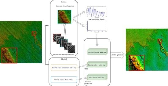
We analyzed the inherent characteristics of mixed errors in local areas for modeling the errors to resolve the problem of mixed errors in DEM data and used variational ideas to constrain the gradient direction of DEM data to avoid redundant elimination. Transforming invariant low-rank textures can transform multidirectional errors, so sparse low-rank mixed-error structures can be better represented, and nonlocal self-similarity was used to remove random noise. Finally, the proposed recovery model used an algorithm based on alternating directions of the multiplier. The proposed low-rank group-sparse method (LRGS) removes mixing errors better than the most recent processing methods and existing dataset products. The main contributions of this study are:

• The discovery of the inherent characteristics of mixed errors in local areas for extracting the low-rank sparse structure of multidirectional stripe errors while unifying the nonlocal sparsity of random noise to eliminate mixing errors;
• The proposal of an algorithm based on alternating directions of the multiplier to ensure the convergence of the proposed recovery model.

Section 2 introduces the relevant characteristics of mixed errors, a theoretical DEM model and the proposed method and its optimization. Section 3 compares LRGS with some existing methods of error removal and mainstream public data sets. Section 4 discusses and analyses the effect of this method on further data-based research. Section 5 provides a summary.

2. Materials and Methods

2.1. Materials

We used the SRTM 1 data downloaded from (https://e4ftl01.cr.usgs.gov/MEASURES/SRTMGL1.003/2000.02.11/, accessed on 30 March 2021) as the experimental data set (There are 14,520 block files in total, each data block was a 3601 × 3601 grid, the data range is between 56 degrees south latitude and 61 degrees north latitude, including 12,967,201 integers (int) type heights and information for longitude and latitude).

The selection of experimental areas considered a variety of terrains, including valley basin area, rugged scenery, flat areas or man-made structures, the terrain of some experimental areas is shown in Figure 2. A detailed introduction of the reasons for selecting the experimental areas and the experimental design is in Section 2.6.

2.2. Features of Mixed Errors

SRTM1 data represent the digital simulation of terrain surfaces using discrete elevated points collected by radar, i.e., the spatial distribution of the actual terrain features in digital form based on the spatial grid structure [27]. The data block of each arc second of SRTM1 can, therefore, be approximated as an image, with longitude and latitude as coordinates and height as coordinate values, which motivated us to explore the characteristics of mixed-error structures using the idea of image fields.

The abnormal vibration of satellite radar during data acquisition will add mixed errors to the data, thereby disturbing the normal data. Previous studies have investigated the causes and characteristics of mixed errors. For example, Crippen et al. [28] found that stripe errors were regular fluctuations in height, mainly caused by the residual motion errors of the interferometry mast, and the stripe errors were mainly concentrated in the northeast to southwest and northwest to southeast directions because the mast was a fixed structure. This example indicates that stripe errors have clear distributional ranges, so they have sparse characteristics in local areas. The change in elevation caused by the interferometer has an approximate value in an adjacent area, which can be regarded as a systematic error so that the low-rank characteristic of an error (Section 2.4) can be separated from the normal data.

Spike errors are usually distributed in flat areas, mainly because changes in the surface reflectance of flat terrain will cause random errors [4], allowing us to treat spike errors as random noise for separation using nonlocal similarity (Section 2.4). In addition, spike errors will inevitably affect the low rank of the elevation of local areas, and eliminating the errors is beneficial to the low-rank characteristic expression of the stripe errors in the same area.

Data for terrain gradients are very sensitive to sudden changes in height in the DEM [29], indicating that similar indicators based on the first or second derivative of the elevation of the DEM surface, such as slope and surface curvature, are particularly affected by the spatial autocorrelation of mixing errors in the DEM. Analyzing the gradient decomposition in Figure 3 indicates that the regular distribution stripes mainly affected the data for an elevational gradient in the direction orthogonal to it, and Figure 4 indicates that mixed errors interfered with the data in both gradient directions. Interestingly, the horizontal gradients and slopes in the DEM data set were particularly sensitive to mixed errors [1], providing us with relevant, reliable features for regularizing constraints (Section 2.4).

2.3. Model of Data Structure

Given the coordinates of longitude and latitude ($L$ and $B$) in the DEM and the corresponding discrete point elevations E, the data set can be represented by:

$$R=(B,L,E_{BL}),$$

(1)

where $R$ is the data set, $L$ and $B$ are the longitude and latitude of the corresponding grid and $E_{BL}$ is the elevation at the corresponding longitude and latitude. We describe a structure model that includes random noise and systematic errors based on the superimposed form of mixed error as:

$$E(B,L)=T(B,L)+e(B,L,T(B,L))\hspace{1em}\hspace{1em}(E,T,e\in R^{M\times N}),$$

(2)

where $E(B,L)$ is the data containing the mixed error, $T(B,L)$ is the clean height at the corresponding longitude and latitude and $e(B,L,T(B,L))$ is the mixed-error component. The stripe error in the mixed error is correlated with the normal data in the direction of the tangent of the stripe, so the mixed error can be written as:

$$e(B,L,T(B,L))=S(B,L,T(B,L))+N(B,L)\hspace{1em}\hspace{1em}(e,S,N\in R^{M\times N}),$$

(3)

where $S(B,L,T(B,L))$ is the stripe error associated with $T(B,L)$ and $N(B,L)$ is the random noise. The data-structure model can, therefore, be expressed as:

$$E(B,L)=T(B,L)+S(B,L,T(B,L))+N(B,L)\hspace{1em}\hspace{1em}(E,T,S,N\in R^{M\times N}),$$

(4)

2.4. Local Low-Rank Sparse Regularization

Clean data have global low-rank characteristics because the stripe structure in the local range is similar to the line structure (Figure 4), so the rank of the matrix is near 1. The effect of low-rank regularization will, therefore, be better for local stripes.

Stripe errors of multidirectional mixing, however, destroy their low-ranking characteristics in real cases, so the errors cannot be easily recognized. We thus recovered the low-rank features of the stripe texture using:

$$\begin{gathered} S:R^{M\times N}\to R^{M\times N}:S^l({\tau }^{-1}) \\ S(B,L)=S^l\circ {\tau }^{-1}(B,L)=S^l({\tau }^{-1}(B,L)), \end{gathered}$$

(5)

where $S^l$ is the restored low-rank texture, $R^{M\times N}$ is the data domain, which is unchanged after restoration, and $\tau$ is a transformation factor [30].

The low-rank features of the local texture were recovered, but sparse random noise was also mixed into the local data. Different latitudes and longitudes contain similar terrains, such as flat, undulating and detailed-edge terrain. These similar structures have similar elevations in the data, i.e., the information of the DEM is redundant, so nonlocal regions in the DEM are strongly correlated. That is, the elevations are similar in nonlocal regions, which motivated us to use nonlocal self-similarity to perform block searches while recovering the low rank of the texture, thereby eliminating sparsely distributed random noise.

The local-error matrix model can thus be expressed as: $S\circ \tau =S^l+N$, where $S^l$ is a low-rank matrix, $N$ is random noise and to recover $S^l$ is a two-objective optimization problem:

$$\underset{S^0,N}{min}(rank(S^l),||N|{|}_0)\hspace{1em}\hspace{1em}s.t.S\circ \tau =S^l+N,$$

(6)

Equation (6) is a non-deterministic polynomial complete (NP)-hard problem, so it can be relaxed to a problem of single-objective convex optimization:

$$\underset{S^0,N}{min}||S^l{||}_{\ast }+\lambda ||S\circ \tau -S^l|{|}_1\hspace{1em}\hspace{1em}s.t.S\circ \tau =S^l+N,$$

(7)

This problem is typical of low-rank matrix approximation. $||S^l{||}_{\ast }$ represents the nuclear norm of the low-rank texture matrix, $||S\circ \tau -S^l|{|}_1$ is the $L_1$ norm of random noise and $\lambda$ is the weight parameter. We will unify this problem in Section 2.5 and solve it using an alternating-direction multiplier algorithm.

For the local low-rank matrix after the low-rank feature recovery, the 2-norm values in the striped column and the unstriped column in the local region have obvious peak-to-valley contrasts, so the stripes have the characteristics of local group sparsity (Figure 4). The local-stripes component is thus constrained to $||S^l{||}_{2,1}$, where ${||||}_{2,1}$ is the $L_{2,1}$ norm and $||S^l{||}_{2,1}={\displaystyle \sum _{j=1}^n||S_j^l|{|}_2}={\displaystyle \sum _{j=1}^n\sqrt{{\displaystyle \sum _{i=1}^m|s_{ij}^l{|}^2}}}$, i.e., we can find the $L_1$ norm for the two norms of each column vector of the matrix.

Figure 3 shows the horizontal and vertical gradients of the data when the low-rank texture is restored. As mentioned in Section 2.2, the stripes will badly destroy the gradient changes in the direction of the horizontal gradient of the terrain data but will have little effect on the direction of the vertical gradient. The component of the local mixing error is also mainly concentrated in the direction of the vertical gradient. We, therefore, only focused on the sparse changes in the direction of the horizontal gradient of the potential T and the vertical-gradient direction of the local error. The regular terms could be expressed as: $||{\nabla }_{x}T|{|}_1$ and $||{\nabla }_y(S\circ \tau ){||}_1$.

2.5. Proposed Model and Optimization

Combining all the terms of regularization in Section 2.4, our proposed model becomes:

$$\begin{array}{l}\underset{T,S,N}{argmin}{\lambda }_1(||S^l{||}_{\ast }+\lambda ||S\circ \tau -S^l|{|}_1)+{\lambda }_2||S^l{||}_{2,1}+{\lambda }_3||{\nabla }_y(S\circ \tau ){||}_1+{\lambda }_4||{\nabla }_{x}T|{|}_1\\ +\frac{1}{2}||E-T-S{||}_F^2\end{array},$$

(8)

To find the globally optimal solution, we first constructed the auxiliary variables $R=S^l$, $Y=S\circ \tau -S^l$, $U=S^l$, $H={\nabla }_y(S\circ \tau )$ and $P={\nabla }_{x}T$ to transform the model into a problem of constraint:

$$\begin{array}{l}\underset{R,Y,U,H,P,T,S}{argmin}{\lambda }_1(||R{||}_{\ast }+\lambda ||Y|{|}_1)+{\lambda }_2||U{||}_{2,1}+{\lambda }_3||H{||}_1+{\lambda }_4||P|{|}_1+\frac{1}{2}||E-T-S{||}_F^2\\ subjecttoR=S^l,Y=S\circ \tau -S^l,U=S^l,H={\nabla }_y(S\circ \tau ),P={\nabla }_{x}T\end{array},$$

(9)

where ${\lambda }_1$, $\lambda$, ${\lambda }_2$, ${\lambda }_3$ and ${\lambda }_4$ are positive regularization parameters, $||S^l{||}_{\ast }$, $||S^l{||}_{2,1}$ and $||{\nabla }_y(S\circ \tau ){||}_1$ are the low-rank, group-sparse and direction regularizations of the stripe error, respectively, $||S\circ \tau -S^l|{|}_1$ is the random-noise sparse regularization, $||{\nabla }_{x}T|{|}_1$ is the direction regularization of clean elevation data, and $\frac{1}{2}||E-T-S{||}_F^2$ is a term of data fidelity.

The corresponding augmented Lagrangian function is:

$$\begin{array}{l}L(R,U,H,P,T,S,C)={\lambda }_1||R_Y{||}_{\ast }+{\lambda }_2||U{||}_{2,1}+{\lambda }_3||H{||}_1+{\lambda }_4||P|{|}_1+\frac{1}{2}||E-T-S{||}_F^2\\ +\frac{k_1}{2}||S\circ \tau -R_Y+\frac{C_1}{k_1}{||}_F^2+\frac{k_2}{2}||S^l-U+\frac{C_2}{k_2}{||}_F^2+\frac{k_3}{2}||{\nabla }_y(S\circ \tau )-H+\frac{C_3}{k_3}{||}_F^2\\ +\frac{k_4}{2}||{\nabla }_{x}T-P+\frac{C_4}{k_4}{||}_F^2\end{array},$$

(10)

where C is the Lagrangian multiplier, k is the positive penalty parameter and $R_Y=||R{||}_{\ast }+\lambda ||Y|{|}_1$. The $L_1$ regularization term in the model has an absolute value and is discontinuous and not differentiable at the sharp points, so it is difficult to solve directly. We, therefore, used the alternating-direction multiplier method (ADMM) [31] to combine the advantages of the dual-decomposition method and the enhanced Lagrangian method for constraint optimization. Integrating the overall steps, the error elimination algorithm based on the ADMM solution is presented in Algorithm 1:

Algorithm 1 ADMM-based error elimination

Input$:\mathrm{Initial}\mathrm{source}\mathrm{data}E,\mathrm{set}\mathrm{regularization}\mathrm{parameter}{\lambda }_1\dots {\lambda }_4>0,\mathrm{penalty}\mathrm{parameter}{k}_1\dots k_4>0$

1: initialization: $T^0$, $S^0$, $R_Y^0$, $U^0$, $H^0$, $P^0$, $\tau$, $\mu$, $\mathrm{Lagrangian}\mathrm{multiplier}{C}_1\dots C_4=0$

2: While does not converge do

3:              Update $R_Y^{n+1}$, $U^{n+1}$, $H^{n+1}$, $P^{n+1}$:

4:                         $R_Y^{n+1}\leftarrow \underset{R_Y}{arcmin}\frac{2{\lambda }_1}{k_1}\parallel R_Y|{|}_{\omega ,\ast }+\parallel S\circ \tau -R_Y+\frac{C_1}{k_1}|{|}_F^2$ by Equation (13)

5:                         $U_i^{n+1}\leftarrow \underset{U}{arcmin}{\displaystyle {\sum }_{i=1}^m[{\lambda }_2\parallel U_i^n|{|}_2+\frac{k_2}{2}\parallel {(S^l)}_i^n-U_i^n+\frac{{(C_2^n)}_i}{k_2}|{|}_F^2]}$ by Equation (15)

6:                         $H^{n+1}\leftarrow \underset{H}{arcmin}{\lambda }_3\parallel H|{|}_1+\frac{k_3}{2}\parallel {▽}_y(S\circ \tau )-H+\frac{C_3}{k_3}|{|}_F^2$ by Equation (17)

7:                         $P^{n+1}\leftarrow \underset{P}{arcmin}{\lambda }_4\parallel P|{|}_1+\frac{k_4}{2}\parallel {▽}_{x}T-P+\frac{C_4}{k_4}|{|}_F^2$ by Equation (19)

8:              Update $T^{n+1}$, $S^{n+1}$:

9:        $(T^{n+1},S^{n+1})\leftarrow \underset{T,S}{arcmin}\frac{1}{2}\parallel E-T-S|{|}_F^2+\frac{k_1}{2}\parallel S\circ \tau -R_Y+\frac{C_1}{k_1}|{|}_F^2+\frac{k_2}{2}\parallel (S^l)-U+\frac{C_2}{k_2}|{|}_F^2$

$+\frac{k_3}{2}\parallel {▽}_y(S\circ \tau )-H+\frac{C_3}{k_3}|{|}_F^2+\frac{k_4}{2}\parallel {▽}_{x}T-P+\frac{C_4}{k_4}|{|}_F^2$ by Equation (21)

10:              $\mathit{Update}\mathrm{Lagrangian}\mathrm{multiplier}{C}_1$, $C_2$, $C_3$, $C_4$:

11:                         $C_1^{m+1}=C_1^m+k_1({(S^l)}^{m+1}-R_Y^{m+1})$

12:                         $C_2^{m+1}=C_2^m+k_2({(S^l)}^{m+1}-U^{m+1})$

13:                         $C_3^{m+1}=C_3^m+k_3({▽}_y{(S\circ \tau )}^{m+1}-H^{m+1})$

14:                         $C_4^{m+1}=C_4^m+k_4(({▽}_x{T}^{m+1}-P^{m+1})$

15:              Update $\mathrm{n}=\mathrm{n}+1$, $\mathrm{m}=\mathrm{m}+1$

16:  End while

17: Output: $T,S,N$

The iterative solution in the form of a multiplier for each variable and the Lagrange parameter for the enhanced Lagrangian function are presented below.

The variables are updated and converged in an alternating or sequential manner during the iteration, which can be decomposed into independent subproblems to solve. For the R subproblem:

$$R_Y^{n+1}:=\underset{R}{arcmin}{\lambda }_1||R_Y|{|}_{\ast }+\frac{k_1}{2}||S\circ \tau -R_Y+\frac{C_1}{k_1}{||}_F^2,$$

(11)

This problem is typical for low-rank matrix approximation. The weighted nuclear norm can adapt to varying error levels for obtaining better results to the problem of minimizing the nuclear norm:

$$R_Y^{n+1}:=\underset{R}{arcmin}{\lambda }_1||R_Y|{|}_{w,\ast }+\frac{k_1}{2}||S\circ \tau -R_Y+\frac{C_1}{k_1}{||}_F^2,$$

(12)

where Gu, S. et al. [32] proposed that $||R_Y|{|}_{w,\ast }={{\displaystyle {\sum }_i^{}|w_i{\sigma }_i(R_Y)|}}_1$ is the weighted nuclear norm and $w_i=\frac{c\sqrt{n}}{{\sigma }_i(R)+\epsilon }$ is the adaptive weight, $c$ is a positive number, $n$ is the number of matches of similar patches and $\epsilon$ is a small positive value, which can avoid zeros for singular values that cause the denominator to be zero.

This problem can be solved using a singular-value threshold algorithm [33] to minimize the nuclear norm because multiplying the objective function by a constant coefficient does not affect the acquisition of the minimum extreme point. Performing a soft-threshold operation on the singular-value matrix, we get:

$$D_{{\lambda }_1}(R_Y^{n+1})=U^n{D}_{{\lambda }_1}({\sigma }_{{\displaystyle \sum }}){(V^n)}^{\ast },$$

(13)

where according to the soft threshold algorithm proposed by Wright, S.J. et al. [34], $D_{{\lambda }_1}({\sigma }_{{\displaystyle \sum }})$ can be written as $D_{{\lambda }_1}({\sigma }_{{\displaystyle \sum }})=\mathrm{sign}({\sigma }_{{\displaystyle \sum }})max\left\{{\sigma }_{{\displaystyle {\sum }_{ii}}}-\frac{2{\lambda }_1}{k_1},0\right\}$ and ${\sigma }_{{\displaystyle {\sum }_{ii}}}$ are diagonal elements of the singular value matrix.

For the U subproblem:

$$U^{n+1}:=\underset{U}{arcmin}{\lambda }_2||U{||}_{2,1}+\frac{k_2}{2}||S^l-U+\frac{C_2}{k_2}{||}_F^2,$$

(14)

The problem of group-sparse minimization can become a problem of suboptimization.

That is, the group-sparse minimization problem is solved in groups, and the closed-form solution of each group using the soft threshold is:

$$\begin{array}{l}{U}_i^{n+1}=\mathrm{sign}(||S_i^l-U_i^n+\frac{(C_2^n{)}_i}{k_2}|{|}_2)·\\ \mathrm{m}\mathrm{a}\mathrm{x}\left\{||S_i^l-U_i^n+\frac{(C_2^n{)}_i}{k_2}|{|}_2-\frac{2{\lambda }_2}{k_2},0\right\}\frac{S_i^l-U_i^n+\frac{(C_2^n{)}_i}{k_2}}{||S_i^l-U_i^n+\frac{(C_2^n{)}_i}{k_2}|{|}_2}\end{array},$$

(15)

where $i$ is the ith group, and the sign is a signum function.

The H subproblem can be solved using threshold shrinkage:

$$H^{n+1}:=\underset{H}{arcmin}{\lambda }_3||H{||}_1+\frac{k_3}{2}||{\nabla }_y(S\circ \tau )-H+\frac{C_3}{k_3}{||}_F^2,$$

(16)

$$H^{n+1}=soft({\nabla }_y(S\circ \tau {)}^n+\frac{C_3^n}{k_3},\frac{{\lambda }_3}{k_3}),$$

(17)

The P subproblem can also be effectively solved using the soft threshold formula in Equation (19):

$$P^{n+1}:=\underset{P}{arcmin}{\lambda }_4||P|{|}_1+\frac{k_4}{2}||{\nabla }_{x}T-P+\frac{C_4}{k_4}{||}_F^2,$$

(18)

$$P^{n+1}=soft({\nabla }_x{T}^n+\frac{C_4^n}{k_4},\frac{{\lambda }_4}{k_4}),$$

(19)

For the (T, S) subproblem:

$$\begin{array}{l}(T^{n+1},S^{n+1}):=\underset{T,S}{arcmin}\frac{1}{2}||E-T-S{||}_F^2+\frac{k_1}{2}||S\circ \tau -R_Y+\frac{C_1}{k_1}{||}_F^2+\frac{k_2}{2}||S^l-U+\frac{C_2}{k_2}{||}_F^2\\ +\frac{k_3}{2}||{\nabla }_y(S\circ \tau )-H+\frac{C_3}{k_3}{||}_F^2+\frac{k_4}{2}||{\nabla }_{x}T-P+\frac{C_4}{k_4}{||}_F^2\end{array},$$

(20)

This problem is a problem of least-squares quadratic optimization [35] and has a closed-form solution. The explicit solution is:

$$\{\begin{array}{c}(k_4{\nabla }_x^T{\nabla }_x+I)T=k_4{\nabla }_x^T{P}^{n+1}-\frac{C_4^n}{2}+E-IS\\ \begin{array}{c}(k_1+k_2+k_3{\nabla }_y^T{\nabla }_y+I)S=k_1{\tau }^{-1}\circ R_Y^{n+1}-\frac{{\tau }^{-1}\circ C_1^n}{2}+k_2{U}^{n+1}-\frac{C_2^n}{2}+k_3{\nabla }_y^T{\tau }^{-1}\circ \\ H^{n+1}-\frac{{\tau }^{-1}\circ C_3^n}{2}+E-IT\end{array}\end{array},$$

(21)

We can efficiently calculate this solution in the Fourier domain, and the difference operator can be solved using fast Fourier transformation.

Finally, updated the Lagrange multipliers $C_1^{}$, $C_2^{}$, $C_3^{}$ and $C_4^{}$.

2.6. Experimental Design and Quantitative Assessments

The proposed algorithm was applied to include the severe mixed-error areas S31E147, S35E144, S36E144 and N01E012, and shows the processing situation of local enlargement areas, including a valley basin area, rugged scenery, flat areas or man-made structures to illustrate the improvement of visual quality.

In the simulation experiment, we selected the N01E12 area, which has an elevation range of 456–950 m, with more textural details and rugged landscape, and the elevation information was not disturbed by errors. The local enlargement area selection includes a valley basin area with a vertical drop of about 300 m and a rugged terrain with an elevation range of about 625–700 m that contains more texture details. The selection of the local expansion area considers the effect of eliminating the mixing error in the mountainous and rugged terrain and the effect of preservation of terrain details. LRGS was tested by adding a mixed error of two stripe directions and random noise. We set the stripe error to random intensity, width and distribution and added global random noise to simulate the complex situation of errors in real data. The degraded data for elevation generated was of double type.

In the real experiment, the area’s selection mainly considered the effect compared with the Gallant data set, which is the official version of the Australian government for error elimination. In addition to comparison with existing algorithms, comparison with publicly released official data sets can better reflect the true situation of data processing. We selected the areas S31E147, S35E144 and S36E144 with real mixed errors in the SRTM1 data set, including problems of cross-direction oblique stripes and random noise to test LRGS. The selection of the local magnification area takes into account the man-made buildings and the small structure of the flat area in order to show the processing effect from the detailed microscopic perspective.

LRGS was compared to several mainstream denoising methods: low-pass filtering (LF), Total Variation (TV) [25], Unidirectional Total Variation (UTV) [26], Low-Rank based Single-Image Decomposition (LRSID) [22] and the Gallant data set (http://nedf.ga.gov.au, accessed on 30 March 2021). We used the quantitative evaluation indicators root-mean-squared error (RMSE), peak signal-to-noise ratio (PSNR), structural similarity index (SSIM) and mean cross-track profiles. The square of the F-norm of the difference between the original elevation and the recovered elevation is the mean square error between the original and recovered data, so the PSNR evaluation index suitable for the data in this study is:

$$MSE=\frac{1}{mn}||E-T{||}_F^2=\frac{1}{mn}{\displaystyle \sum _{i=0}^{m-1}{\displaystyle \sum _{j=0}^{n-1}{[E(x_i,y_j)-T(x_i,y_j)]}^2}},$$

(22)

$$PSNR=20\times {\log }_{10}(MA{X}_E^{})-10\times {\log }_{10}(MSE),$$

(23)

where $MSE$ represents the mean square error of the elevations between the original data $E$ and the recovered data $T$ and $MA{X}_E^{}$ represents the maximum elevation in the original data, which was changed based on the range of elevations of different data. The larger the value, the smaller the distortion of the data.

The SSIM equation is:

$$l(E_1,E_2)=\frac{2{\mu }_1{\mu }_2+C_1}{{\mu }_1^2+{\mu }_2^2+C_1}\hspace{1em}c(E_1,E_2)=\frac{2{\sigma }_1{\sigma }_2+C_2}{{\sigma }_1^2+{\sigma }_2^2+C_2}\hspace{1em}s(E_1,E_2)=\frac{{\sigma }_{12}+C_3}{{\sigma }_1{\sigma }_2+C_3},$$

(24)

$$SSIM(E_1,E_2)=l(E_1,E_2)·c(E_1,E_2)·s(E_1,E_2),$$

(25)

where ${\mu }_1$ and ${\mu }_2$ represent the mean elevations in the data matrices $E_1$ and $E_2$, respectively, ${\sigma }_1$ and ${\sigma }_2$ represent the elevation variances of the data matrices $E_1$ and $E_2$, respectively, ${\sigma }_{12}$ represents the elevation covariance of the data matrices $E_1$ and $E_2$ and $C_1$, $C_2$ and $C_3$ are constants, usually $C_1=(K_{1}L{)}^2$, $C_2=(K_{2}L{)}^2$ and $C_3=C_2/2$, and generally $K_1=0.01$ and $K_2=0.03$. The value of $L$ depends on the range of elevations in these data matrices. The range of the SSIM value is [0, 1]. The larger the value, the smaller the distortion of the data.

3. Results

3.1. Simulated Experiments

The results of the various methods to remove the vertical stripes and random-noise mixing errors are shown in Figure 5 and Figure 6 is a partially enlarged view.

From the point of view of visual evaluation, the low-pass filter in Figure 6c blurred the data image and lost the detailed structure while filtering out the mixing errors, and ringing occurred at the edge because the transition characteristic of the ideal low-pass filter was too steep (Figure 5c). TV performed well globally and substantially suppressed random noise (Figure 5d), but the detail was lost after zooming in locally (Figure 6d). UTV removed the obvious stripe structure but could not effectively remove the existing random noise and had a specific impact on the structure of the data image (Figure 6e). LRSID completely removed the vertical-stripe structure and preserved the data structure well (Figure 6f). LRSID also had a specific suppressive effect on random noise, but some random noise remained. Our method showed better results in removed, mixed errors and retained details (Figure 6g).

From the point of view of quantitative evaluation, our method is in RMSE, PSNR and the SSIM indicators all had better data-reduction and structure-retention capabilities (

Table 1. Results of the peak signal-to-noise ratio (PSNR) and structural similarity index (SSIM) simulation experiments.

		Add	LF	TV	UTV	LRSID	LRGS
Figure 5	RMSE (m)	30.027	33.006	27.539	30.234	28.467	26.980
	PSNR (dB)	30.013	29.191	30.764	29.953	30.476	30.942
	SSIM	0.5511	0.4322	0.5460	0.5179	0.6617	0.8319
Figure 7	RMSE (m)	30.581	33.249	27.8761	30.855	29.191	28.062
	PSNR (dB)	29.854	29.127	30.659	29.776	30.258	30.601
	SSIM	0.5370	0.4297	0.5400	0.5013	0.6259	0.7213

), bold font represents the best-performing method in each quantitative evaluation index.

It is worth noting that in the quantitative evaluation of Figure 7, the TV algorithm is slightly better than the LRGS algorithm in terms of RMSE and peak signal-to-noise ratio.

However, in combination with structural similarity, it can be found that the TV algorithm’s ability to retain detailed structures is not excellent. This is mainly due to its smoothing feature, which makes it excellent in random noise suppression, but it is not excellent in preserving the structure and eliminating system errors, which is consistent with the conclusions of the visual assessment.

The results of the various methods for removing the mixing error of oblique stripes and random noise are shown in Figure 7 and Figure 8 shows a partially enlarged view.

From the point of view of visual evaluation, the data image had problems of blurring and loss of detail, although the low-pass filter and TV obviously suppressed random noise (Figure 8e,f). UTV and LRSID did not obviously remove oblique stripes, and random noise could not be completely removed. UTV also affected the data structure. Our method effectively removed oblique stripes and random noise and recovered the detailed structure well (Figure 7g, Table 1).

3.2. Real Experiments

Figure 9 show the effect of processing using various methods on real area S31E147 for visual evaluation. Figure 10 show partial enlargements of the corresponding data.

As an example, the low-pass filtering in Figure 10a over-smoothed the complex superposition of errors in the data under real conditions, and many details of the image were lost (Figure 10b). TV suppressed random noise very well, but streak errors remained, and the detailed structure of the house was lost (Figure 10c). UTV and LRSID could not effectively eliminate the effect of oblique cross stripes and superimposed random noise but preserved the detailed structure well (Figure 10d,e). Many details of the Gallant data set were lost, and over-smoothing occurred, but the hydrological structure was enhanced (Figure 10f). Our method was better at eliminating mixed errors and retaining the detailed structure covered by mixed errors (Figure 10g).

Figure 11 shows the mean cross-track profiles of the data for quantitative evaluation, using area S31E147 in Figure 9 as an example. The local enlargement is shown in the lower-right corner to better illustrate the details of the curve.

The dense spikes in area S31E147 were due to the effects of mixing errors (Figure 11a). The local zoom indicated that our method removed the spikes well, indicating that the mixing errors had been eliminated from the data and the curve fluctuations were well preserved, so the structure and elevations of the data image were well preserved (Figure 11f). Low-pass filtering was destroyed due to the ringing phenomenon at the edge, and the elevation data and data structure were destroyed (Figure 11b–e,g). TV produced a smooth curve, indicating that the detailed structure was lost to some extent, and UTV and LRSID did not obviously affect the removal of spikes, which led to residual stripes and random noise. The Gallant data set clearly deviated from the original range of the curve, and the curve was over-smoothed.

Figure 12 show the effect of processing using various methods on real area S35E144 for visual evaluation. Figure 13 show partial enlargements of the corresponding data.

Figure 14 show the effect of processing using various methods on real area S36E144 for visual evaluation. Figure 15 show partial enlargements of the corresponding data.

4. Discussion

Our study found multiple classifications of mixed errors in the data for global elevation, mainly in two aspects, systematic errors and random noise specifically manifested as multidirectional stripe errors and spikes and speckle problems. Systematic errors can be regularized by mining features, and random noise can be solved by nonlocal self-similarity. We initially decided to represent the direction of multidirectional stripes globally in order to use the group-sparse features, but the effect was not ideal due to multidirectional mixing. We, therefore, conducted experiments and found that the low-rank direction of the local region of the data was unique and that the low-rankness and group-sparseness characteristics of local mixing errors were better (Figure 4). We decomposed the global multidirectional errors into local unidirectional processing and concurrently dealt with random noise in order to remove interference and better indicate the sparse local characteristics of the error. Our experiments also found that the single-direction stripe errors interfered greatly with the elevation of the intersecting direction for the over-smoothing phenomenon that occurred after data processing in previous studies but had little effect on the elevation in the same direction (Figure 3). Processing in both directions would, therefore, lead to excessive elimination and smoothing, so we restricted the processing to the elevation data in the direction that intersected the error.

The gradient of the elevation data was substantially improved both visually and quantitatively after eliminating the mixing errors when analyzing the effect of mixing errors on the direction of the data gradient in Figure 4, mainly because the gradient data were very sensitive to sudden changes in elevation in the DEM [29]. Similar research on the first or second derivatives based on DEM surface elevations, such as slope, surface curvature and other calculated values, will, therefore, be greatly improved.

We demonstrated the gradient changes and the local 3Dmodel of the data (Figure 16). Data containing mixed errors would badly interfere with the calculation of the relevant parameters based on the data, which would be represented as fringe and spike problems in the model. This method would, therefore, have specific applications to any further scientific research based on data or images.

Using this method to process global SRTM 1 data and releasing a new data set will be our next goals.

5. Conclusions

We analyzed the inherent features of local mixing errors for modeling local low-rank sparse regularization to remove the problem of mixing errors, which involved two considerations. First, we used the uniqueness of the low-rank transformation of the local data direction to represent the local low-rank error structure, used variational ideas and group sparseness to constrain the strip components and constrained the gradient direction of the data to avoid redundancy elimination. The nonlocal self-similarity of random noise was also used to eliminate random noise. Second, the proposed model was solved using the alternating-direction multiplier method. This method eliminated mixing errors better than the most recent processing methods and existing dataset products.

References

- Hirt, C. Artefact detection in global digital elevation models (DEMs): The Maximum Slope Approach and its application for complete screening of the SRTM v4.1 and MERIT DEMs. Remote Sens. Environ. 2018, 207, 27–41. [Google Scholar] [CrossRef] [Green Version]
- Li, Z.; Zhu, C.; Gold, C. Digital Terrain Modeling: Principles and Methodology; CRC Press: Boca Raton, FL, USA, 2005. [Google Scholar]
- Yamazaki, D.; Ikeshima, D.; Tawatari, R.; Yamaguchi, T.; O’Loughlin, F.; Neal, J.C.; Sampson, C.C.; Kanae, S.; Bates, P.D. A high-accuracy map of global terrain elevations. Geophys. Res. Lett. 2017, 44, 5844–5853. [Google Scholar] [CrossRef] [Green Version]
- Takaku, J.; Iwasaki, A.; Tadono, T. Adaptive filter for improving quality of ALOS PRISM DSM. In Proceedings of the 36th IEEE International Geoscience and Remote Sensing Symposium, IGARSS 2016, Beijing, China, 10–15 July 2016; pp. 5370–5373. [Google Scholar]
- Rodriguez, E.; Morris, C.S.; Belz, J.E.J.P.E.; Sensing, R. A global assessment of the SRTM performance. Photogramm. Eng. Remote. Sens. 2006, 72, 249–260. [Google Scholar] [CrossRef] [Green Version]
- Gallant, J. Adaptive smoothing for noisy DEMs. Geomorphometry. Available online: http://geomorphometry.org/Gallant2011 (accessed on 7 September 2011).
- Simard, M.; Zhang, K.; Rivera-Monroy, V.H.; Ross, M.S.; Ruiz, P.L.; Castaneda-Moya, E.; Twilley, R.R.; Rodriguez, E. Mapping height and biomass of mangrove forests in Everglades National Park with SRTM elevation data. Photogramm. Eng. Remote Sens. 2006, 72, 299–311. [Google Scholar] [CrossRef]
- Oimoen, M.J. An effective filter for removal of production artifacts in US Geological Survey 7.5-minute digital elevation models. In Proceedings of the Fourteenth International Conference on Applied Geologic Remote Sensing, Las Vegas, NV, USA, 6–8 November 2000; pp. 6–8. [Google Scholar]
- Gallant, J.C.; Read, A.M. A near-Global Bare-Earth Dem from Srtm. ISPRS Int. Arch. Photogramm. Remote Sens. Spat. Inf. Sci. 2016, XLI-B4, 137–141. [Google Scholar] [CrossRef]
- Real, V.; Lucas, C. A Novel Noise Removal Algorithm for Vertical Artifacts in Digital Elevation Models. In Proceedings of the 34th Asian Conference on Remote Sensing (ACRS), São Paulo, Brazil, 20–24 October 2013; pp. 20–24. [Google Scholar]
- Lewington, E.L.M.; Livingstone, S.J.; Sole, A.J.; Clark, C.D.; Ng, F.S.L. An automated method for mapping geomorphological expressions of former subglacial meltwater pathways (hummock corridors) from high resolution digital elevation data. Geomorphology 2019, 339, 70–86. [Google Scholar] [CrossRef]
- Kang, W.; Yu, S.; Seo, D.; Jeong, J.; Paik, J. Push-Broom-Type Very High-Resolution Satellite Sensor Data Correction Using Combined Wavelet-Fourier and Multiscale Non-Local Means Filtering. Sensors 2015, 15, 22826–22853. [Google Scholar] [CrossRef] [Green Version]
- Gallant. 1secSRTM Derived DEMs UserGuide v1.0.4; Geoscience Australia, Symonston ACT: Canberra, Australia, 2011.
- Jiang, T.X.; Huang, T.Z.; Zhao, X.L.; Deng, L.J.; Wang, Y. FastDeRain: A Novel Video Rain Streak Removal Method Using Directional Gradient Priors. IEEE Trans. Image Process. 2019, 28, 2089–2102. [Google Scholar] [CrossRef] [Green Version]
- Ng, M.K.; Ngan, H.Y.T.; Yuan, X.M.; Zhang, W.X. Lattice-Based Patterned Fabric Inspection by Using Total Variation with Sparsity and Low-Rank Representations. SIAM J. Imaging Sci. 2017, 10, 2140–2164. [Google Scholar] [CrossRef]
- Cao, J.J.; Wang, N.N.; Zhang, J.; Wen, Z.J.; Li, B.; Liu, X.P. Detection of varied defects in diverse fabric images via modified RPCA with noise term and defect prior. Int. J. Cloth. Sci. Technol. 2016, 28, 516–529. [Google Scholar] [CrossRef]
- Feng, L.L.; Liu, Y.P.; Chen, L.X.; Zhang, X.; Zhu, C. Robust block tensor principal component analysis. Signal Process. 2020, 166, 13. [Google Scholar] [CrossRef]
- Xiaoqun, Z.; Tony, F.C. Wavelet inpainting by nonlocal total variation. Inverse Probl. Imaging 2010, 4, 191–210. [Google Scholar]
- Ortiz, J.D.; Avouris, D.M.; Schiller, S.J.; Luvall, J.C.; Lekki, J.D.; Tokars, R.P.; Anderson, R.C.; Shuchman, R.; Sayers, M.; Becker, R. Evaluating visible derivative spectroscopy by varimax-rotated, principal component analysis of aerial hyperspectral images from the western basin of Lake Erie. J. Gt. Lakes Res. 2019, 45, 522–535. [Google Scholar] [CrossRef]
- Yang, J.H.; Zhao, X.L.; Ma, T.H.; Chen, Y.; Huang, T.Z.; Ding, M. Remote sensing images destriping using unidirectional hybrid total variation and nonconvex low-rank regularization. J. Comput. Appl. Math. 2020, 363, 124–144. [Google Scholar] [CrossRef]
- Chen, Y.; Huang, T.Z.; Zhao, X.L. Destriping of Multispectral Remote Sensing Image Using Low-Rank Tensor Decomposition. IEEE J. Sel. Top. Appl. Earth Observ. Remote Sens. 2018, 11, 4950–4967. [Google Scholar] [CrossRef]
- Chang, Y.; Yan, L.X.; Wu, T.; Zhong, S. Remote Sensing Image Stripe Noise Removal: From Image Decomposition Perspective. IEEE Trans. Geosci. Remote Sens. 2016, 54, 7018–7031. [Google Scholar] [CrossRef]
- Dou, H.X.; Huang, T.Z.; Deng, L.J.; Zhao, X.L.; Huang, J. Directional l(0) Sparse Modeling for Image Stripe Noise Removal. Remote Sens. 2018, 10, 361. [Google Scholar] [CrossRef] [Green Version]
- Jensen, K.H.; Sigworth, F.J.; Brandt, S.S. Removal of Vesicle Structures From Transmission Electron Microscope Images. IEEE Trans. Image Process. 2016, 25, 540–552. [Google Scholar] [CrossRef] [PubMed]
- Xavier, B.; Tony, F.C. Fast dual minimization of the vectorial total variation norm and applications to color image processing. Inverse Probl. Imaging 2008, 2, 455–484. [Google Scholar]
- Bouali, M.; Ladjal, S. Toward Optimal destriping of MODIS data using a unidirectional variational model. IEEE Trans. Geosci. Remote Sens. 2011, 49, 2924–2935. [Google Scholar] [CrossRef]
- Guth, P.L.J.P.E.; Sensing, R. Geomorphometry from SRTM. Photogramm. Eng. Remote Sens. 2006, 72, 269–277. [Google Scholar] [CrossRef]
- Crippen, R.; Buckley, S.; Agram, P.; Belz, E.; Gurrola, E.; Hensley, S.; Kobrick, M.; Lavalle, M.; Martin, J.; Neumann, M.; et al. Nasadem global elevation model: Methods and progress. In Proceedings of the 23rd International Archives of the Photogrammetry, Prague, Czech Republic, 12–19 July 2016; pp. 125–128. [Google Scholar]
- Polidori, L.; El Hage, M.; Valeriano, M.D. Digital Elevation Model Validation with No Ground Control: Application to The Topodata Dem in Brazil. Bol. Cienc. Geod. 2014, 20, 467–479. [Google Scholar] [CrossRef] [Green Version]
- Zhang, Z.D.; Ganesh, A.; Liang, X.; Ma, Y. TILT: Transform Invariant Low-Rank Textures. Int. J. Comput. Vis. 2012, 99, 1–24. [Google Scholar] [CrossRef]
- Eckstein, J.; Bertsekas, D.P. On the Douglas-Rachford Splitting Method And The Proximal Point Algorithm for Maximal Monotone-Operators. Math. Program. 1992, 55, 293–318. [Google Scholar] [CrossRef] [Green Version]
- Gu, S.; Zhang, L.; Zuo, W.; Feng, X. Weighted nuclear norm minimization with application to image denoising. In Proceedings of the 27th IEEE Conference on Computer Vision and Pattern Recognition, CVPR 2014, Columbus, OH, USA, 23–28 June 2014; pp. 2862–2869. [Google Scholar]
- Cai, J.F.; Candes, E.J.; Shen, Z.W. A Singular Value Thresholding Algorithm for Matrix Completion. Siam J. Optim. 2010, 20, 1956–1982. [Google Scholar] [CrossRef]
- Wright, S.J.; Nowak, R.D.; Figueiredo, M.A.T. Sparse Reconstruction by Separable Approximation. IEEE Trans. Signal Process. 2009, 57, 2479–2493. [Google Scholar] [CrossRef] [Green Version]
- Fan, Y.R.; Huang, T.Z.; Liu, J.; Zhao, X.L.J.P.O. Compressive Sensing via Nonlocal Smoothed Rank Function. PLoS ONE 2016, 11, e0162041. [Google Scholar] [CrossRef]
Figure 1.
Area S30E148 in Shuttle Radar Topography Mission 1 (SRTM 1) containing spikes, speckles and multidirectional stripe errors (unit: meter). (a) The original data, (c) the local enlargement of the spike-error area and (e) the local enlargement of the mixed-error area. The second column (b,d,f) contains the data corresponding to panels a, c and e, respectively, after removing the errors using the proposed low-rank group-sparse method (LRGS).
Figure 2.
SRTM 1 data and the terrain of some experimental areas. (a) SRTM 1. Local enlargement of (b) area b, (c) area c, (d) area d marked by the corresponding letters in the figure.
Figure 3.
The interference of stripe errors on different gradient directions. The minimum elevation in this area is 293 m, the maximum elevation is 2000 m, and the maximum elevation difference is 1700 m. Analyzing the gradient decomposition in this rugged landscape, stripes of the regular distribution mainly affected the data for an elevational gradient in the direction orthogonal to it. In this experiment, stripe errors severely interfere with the horizontal gradient of the data. (a) Data with stripe errors, (b) clean data, (c) horizontal gradient of a, (d) vertical gradient of a, (e) horizontal gradient of b, (f) vertical gradient of b, (g) gradient intensity of c, (h) gradient intensity of d, (i) gradient intensity of e and (j) gradient intensity of f.
Figure 4.
Analyzing the gradient decomposition in this experimental area (unit: meter), Mixed noise interferes with data in both gradient directions. The stripe structure in the local range is similar to the line structure, so the rank of the matrix is near 1, and the 2-norm values in the striped column and the unstriped column in the local region have obvious peak-to-valley contrasts. (a) The original Data, local data and mixed errors magnification, (b) processed data, (c) horizontal gradient of original data, (d) vertical gradient of original data, (e) gradient intensity of c, (f) gradient intensity of d, (g) statistics of local mixed errors singular values in a, (h) 2-norm statistics of local mixed errors in a, (i) horizontal gradient of b, (j) vertical gradient of b, (k) gradient intensity of i and (l) gradient intensity of j.
Figure 5.
Results of the simulation experiment for area N01E12 with vertical stripes and random-noise mixing errors (unit: meter). (a) Original N01E12 area (PSNR, SSIM), (b) mixed error (30.01, 0.5511) added, (c) low-pass filter (29.19, 0.4322), (d) total variation (TV) (30.76, 0.5460), (e) Unidirectional Total Variation (UTV) (29.95, 0.5179), (f) Low-Rank based Single-Image Decomposition (LRSID) (30.48, 0.6617) and (g) low rank group-sparse method (LRGS) (30.94, 0.8319).
Figure 6.
Local enlargement of the results of the simulation experiment for area N01E12 (Figure 5). Local enlargements for (a) area N01E12, (b) mixed error added, (c) low-pass filter, (d) TV, (e) UTV, (f) LRSID and (g) LRGS.
Figure 7.
Results of the simulation experiment for area N01E12 with oblique stripes and random-noise mixing errors (unit: meter). (a) Original area N01E12, (b) mixed error added (29.85, 0.5370), (c) low-pass filter (29.13, 0.4297), (d) TV (30.65, 0.5400), (e) UTV (29.78, 0.5013), (f) LRSID (30.26, 0.6259) and (g) LRGS (30.60, 0.7213).
Figure 8.
Local enlargement of the results of the simulation experiment for area N01E12 (Figure 7). Local enlargements for (a) area N01E12, (b) mixed error added, (c) low-pass filter, (d) TV, (e) UTV, (f) LRSID and (g) LRGS.
Figure 9.
Results of the real experiment for area S31E147 (unit: meter). (a) Original S31E147 area, (b) low-pass filter, (c) TV, (d) UTV, (e) LRSID, (f) Gallant and (g) LRGS.
Figure 10.
Results of the real experiment for the local enlargement of area S31E147 (Figure 9). Local enlargements for (a) area S31E147, (b) low-pass filter, (c) TV, (d) UTV, (e) LRSID, (f) Gallant and (g) LRGS.
Figure 11.
Mean cross-track profiles of the results of the real experiment for area S31E147 (unit: meter). (a) Area S31E147, (b) low-pass filter, (c) TV, (d) UTV, (e) LRSID, (f) Gallant and (g) LRGS.
Figure 12.
Results of the real experiment for area S35E144 (unit: meter). (a) Original area S35E144, (b) low-pass filter, (c) TV, (d) UTV, (e) LRSID, (f) Gallant and (g) LRGS.
Figure 13.
Results of the real experiment for the local enlargement of area S35E144 (Figure 12). Local enlargements for (a) area S35E144, (b) low-pass filter, (c) TV, (d) UTV, (e) LRSID, (f) Gallant and (g) LRGS.
Figure 14.
Results of the real experiment for area S36E144 (unit: meter). (a) Original area S36E144, (b) low-pass filter, (c) TV, (d) UTV, (e) LRSID, (f) Gallant and (g) LRGS.
Figure 15.
Results of the real experiment for the local enlargement of area S36E144 (Figure 14). Local enlargements for (a) area S36E144, (b) low-pass filter, (c) TV, (d) UTV, (e) LRSID, (f) Gallant and (g) LRGS.
Figure 16.
The gradient changes and the local 3Dmodel of the data. (a) Horizontal gradient of area S35E144, (b) vertical gradient of area S35E144, (c) horizontal gradient of area S35E144 using the proposed method, (d) vertical gradient of area S35E144 area using the proposed method, (e) local enlargement of area S35E144, (f) local enlargement of area S35E144 area after removing the error using LRGS.