Article

Assessing Vegetation Response to Multi-Scalar Drought across the Mojave, Sonoran, Chihuahuan Deserts and Apache Highlands in the Southwest United States

by
Pratima Khatri-Chhetri
1,*,
Sean M. Hendryx
2,
Kyle A. Hartfield
3,
Michael A. Crimmins
4,
Willem J. D. van Leeuwen
3,5 and
Van R. Kane
1
1
School of Environmental and Forest Sciences, University of Washington, Seattle, WA 98195, USA
2
School of Information, University of Arizona, Tucson, AZ 85721, USA
3
School of Natural Resources and the Environment, University of Arizona, Tucson, AZ 85721, USA
4
Department of Environmental Science, University of Arizona, Tucson, AZ 85721, USA
5
School of Geography, Development and Environment, University of Arizona, Tucson, AZ 85721, USA
*
Author to whom correspondence should be addressed.
Remote Sens. 2021, 13(6), 1103; https://doi.org/10.3390/rs13061103
Submission received: 23 February 2021 / Accepted: 11 March 2021 / Published: 14 March 2021
(This article belongs to the Special Issue Earth Observations for Ecosystem Resilience)

Abstract

:
Understanding the patterns and relationships between vegetation productivity and climatic conditions is essential for predicting the future impacts of climate change. Climate change is altering precipitation patterns and increasing temperatures in the Southwest United States. The large-scale and long-term effects of these changes on vegetation productivity are not well understood. This study investigates the patterns and relationships between seasonal vegetation productivity, represented by Moderate Resolution Imaging Spectroradiometer (MODIS) Normalized Difference Vegetation Index (NDVI), and the Standardized Precipitation Evapotranspiration Index (SPEI) across the Mojave, Sonoran, and Chihuahuan Deserts and the Apache Highlands of the Southwest United States over 16 years from 2000 to 2015. To examine the spatiotemporal gradient and response of vegetation productivity to dry and wet conditions, we evaluated the linear trend of different SPEI timescales and correlations between NDVI and SPEI. We found that all four ecoregions are experiencing more frequent and severe drought conditions in recent years as measured by negative SPEI trends and severe negative SPEI values. We found that changes in NDVI were more strongly correlated with winter rather than summer water availability. Investigating correlations by vegetation type across all four ecoregions, we found that grassland and shrubland productivity were more dependent on summer water availability whereas sparse vegetation and forest productivity were more dependent on winter water availability. Our results can inform resource management and enhance our understanding of vegetation vulnerability to climate change.

Graphical Abstract

1. Introduction

The productivity of vegetation communities is directly impacted by changes in temperature and precipitation, especially in arid and semi-arid regions [1]. In the Southwest United States, for example, the effects of climate change are expected to be pronounced [2]. The frequency, severity, and duration of droughts have increased while water availability has decreased in this region [3]. Trends point to a decline in vegetation productivity due to projected warming and increasingly dry conditions [4,5]. However, the response of desert vegetation productivity to water availability, variations in the timing, and amount of precipitation varies spatially and temporally [2,6]. The need to understand the relationships between vegetation productivity, precipitation, and drought for these desert ecoregions is made more urgent by current and projected global climate change models predicting a general reduction in precipitation and increase in temperatures for these ecoregions [1,3]. With increasingly arid conditions, understanding the vegetation productivity and vegetation types response to different water stress timescales is important to enhance our ability to predict the impact of global change in vegetation [7].
In recent years, a number of studies have focused on the impact of precipitation, temperature, and drought on vegetation at global and regional scales. Global scale studies have shown that decreased photosynthetic activities are correlated with a decrease in the annual precipitation in arid and semi-arid regions [8,9]. Wang et al. [10] found vegetation productivity during the growing season was most highly correlated with precipitation over the preceding 15-months in the Great Plains United States. Similarly, a global study found that vegetation productivity in semi-arid regions around the globe responded to long term drought (8–10 months) [11].
Past research has also studied the response of vegetation productivity to different timescales of seasonal and annual water availability. Normalization of precipitation indices allows identification of variation in drought and resulting water stress from long term means [12]. These variations can be examined at different timescales such as monthly, seasonally, and inter-annually to represent water availability in different reservoirs such as shallow versus deeper soils. Shorter timescales typically show frequent shifts in precipitation relative to the mean and longer periods show fewer but longer duration shifts [12]. For example, vegetation productivity represented by Normalized Difference Vegetation Index (NDVI) was most correlated with short term 3-month drought in the Great Plains [13] and to 1-month drought in semi-arid regions of the Southwest [6] in the United States. Particularly within the Southwest region, studies have found that vegetation productivity in different ecoregions and biomes types are associated with varying time lags of water availability [6,7].
Previous studies have established that the vegetation productivity response to different water stress timescales depends on their physiological structure [11] and biome type [7]. However, previous work has not compared responses of vegetation productivity and drought among deserts with different long-term patterns in the timing and amounts of water availability. In this study, we address this gap by assessing the spatiotemporal response of seasonal vegetation productivity to different water stress (SPEI) timescales. Here, timescale refers to the cumulative water balance over a previous number of months [11] from a measurement of vegetation productivity.
Water stress and vegetation productivity vary both within and between years. These variations can be estimated through remote sensing drought indices such as the Standardized Precipitation Index (SPI) [12] and the recently introduced Standardized Precipitation Evapotranspiration Index (SPEI) [14]. We chose SPEI as a proxy for drought because SPEI uses both precipitation and temperature and has been shown to better reflect the impact of climatic conditions on plants [14]. McClaran and Wei [15] have also shown that SPEI better represents reductions in soil moisture that impact vegetation productivity in the Southwest United States than SPI. Similarly, variations in vegetation productivity can be estimated by remote sensing indices such as the Normalized Difference Vegetation Index (NDVI) [8,16,17]. MODIS NDVI time series data is open-access, globally available, and is not only robust for studying the changes in vegetation across large areas [18] but also very useful for studying insect infestation [19,20], fire detection [21], and the impacts of drought [22,23]. MODIS NDVI data is available at high temporal and 250 m spatial resolution. We chose 16-day MODIS NDVI data for this research.
We analyzed the correlations between NDVI and SPEI across four ecoregions in the Southwest United States to shed new light on the spatiotemporal relationships between vegetation productivity and drought timescales. We analyzed whether general patterns in relationships between vegetation productivity (NDVI) and water availability (SPEI) hold across different desert ecoregions or if the relationships are unique to each. In particular, we examined the impact of different SPEI timescales on NDVI across the Mojave, Sonoran, and Chihuahuan Deserts, and Apache Highlands ecoregions of Southwest United States for 16 years from 2000 to 2015. We also studied the long-term trend and variability of SPEI at different timescales to understand the differences between short- and long-term drought and how this is impacting vegetation productivity. The results of this study are expected to improve our understanding of the spatiotemporal response of vegetation to drought in deserts of the Southwest US and the vulnerability of vegetation to climate change that can be useful in resource management and reducing drought impacts.
Specifically, we ask the following research questions:
  • How do the trends in water availability (SPEI) at different timescales vary by ecoregion?
  • How does vegetation productivity (NDVI) respond to changes in water availability (SPEI)?
    • For each ecoregion, what was the dominant timescale for the relationship?
    • How uniform was the response of NDVI to SPEI across these ecoregions?
    • Does this relationship change by dominant vegetation type?
  • What do these results suggest about plant physiology responses to drought stress in these ecoregions?

2. Materials and Methods
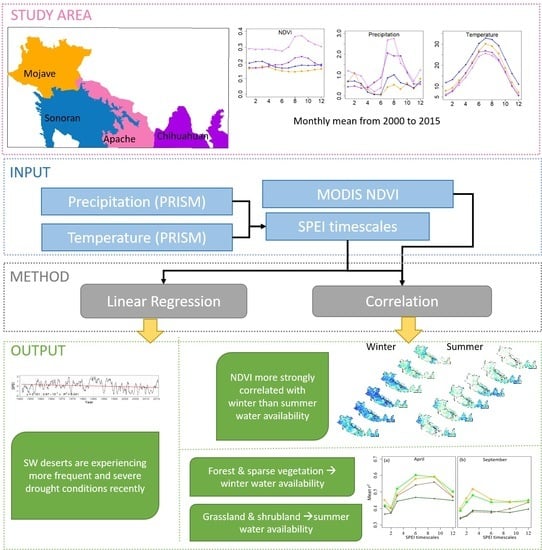
2.1. Study Area

This study was conducted in the Mojave, Sonoran, and Chihuahuan Deserts, and Apache Highlands ecoregions [24] (Figure 1) of the Southwest United States. These ecoregions have some commonalities in terms of aridity and extreme climatic conditions, and differences in terms of elevation, geography, vegetation types, and precipitation patterns. The average summer and winter temperatures of the Sonoran Desert are higher than the other ecoregions (Figure 2) [1]. While on average the Mojave Desert receives the majority of its annual precipitation during the winter-spring season [1,25], the Chihuahuan Desert and Apache Highlands receive precipitation primarily during the summer-monsoon season (Figure 3) [26]. The Sonoran Desert has bimodal precipitation occurring both in the winter and in the summer during the monsoon season. These ecoregions have higher summer precipitation in the east and higher winter precipitation in the west. This difference in precipitation patterns creates an east to west gradient of average seasonal precipitation that creates a distinct climatic regime (Figure 3) [27].
Desert scrub, shrub-steppe, desert grassland, saguaro cacti, and organ pipe cacti are found in these regions [1]. The Mojave Desert consists of perennial vegetation composed mostly of low shrubs; the Sonoran Desert has distinctive vegetation types such as legume trees such as Acacia and mesquite and large cacti at lower elevations and diverse plant communities at higher elevations [27]. The Chihuahuan Desert consists of low shrubs, succulent species, and sparse woodlands at higher elevations and in riparian zones [27]. The Apache Highlands is dominated by woody savannas and closed grasslands [27].
In this study, we focused on April as the representative month of the winter-spring seasons (referred to as ‘winter’) and September as the representative month of the summer monsoon season (referred to as ‘summer’). These representative months were selected based on seasonal peak values in vegetation productivity (NDVI) for each season (Figure 2) to understand the response of seasonal peak NDVI to different SPEI timescales. Similarly, other studies have also used a single month of peak productivity during a growing season to understand the effect of water stress on vegetation during different seasons [7,23].

2.2. Data

2.2.1. Vegetation Productivity (MODIS NDVI)

In this study we derived time series (2000–2015) of biweekly (16-days) composite NDVI data at 250 m resolution from MODIS (MOD13Q1) on the Terra platform [29] from the NASA’s Land Process Distributed Active Archive Center (LP DAAC) at https://lpdaac.usgs.gov/ (accessed on 14 March 2021). We used a 16-day NDVI period to calculate the monthly NDVI values. We took the weighted mean of the 16-day NDVI periods that fell in each month and summed them to get the monthly NDVI. The equation for the weighted mean NDVI for each pixel for each month is given below:
N D V I m o n t h l y = i N D V I i N o .   o f   d a y s   i n   p e r i o d   i   i n   M o n t h N o .   o f   d a y s   i n   M o n t h
where NDVIi is the 16-day composite NDVI value for the period i. The monthly NDVI data was calculated for April and September as the representative months of the winter and summer season, respectively. These months were selected based on seasonal peaks in productivity during each growing season and precipitation patterns in the four ecoregions.

2.2.2. Climate Data (Temperature and Precipitation)

We used monthly precipitation and temperature data modeled at a spatial resolution of 4 km from Oregon State University’s Parameter Regression on Independent Slopes Models (PRISM) for the Conterminous United States (https://prism.oregonstate.edu/recent/ (accessed on 14 March 2021)) from 2000 to 2015 [29]. Monthly precipitation and mean temperature datasets were clipped to the study area and re-projected to the Lambert Azimuth Equal Area projection to match the MODIS NDVI dataset. We used these data to calculate the drought index.

2.2.3. Drought Index (SPEI)

Both precipitation and temperature data were used in calculating the Standardized Precipitation Evapotranspiration Index (SPEI) [14]. The negative SPEI values represent dry conditions and positive SPEI values represent wet conditions. The three main steps for calculating SPEI are as follows: First, Potential Evapotranspiration (PET) is calculated using the Thornthwaite method [30] using temperature as an input. Second, accumulated water balance is calculated by subtracting precipitation from PET at different timescales. Third, the water balance is normalized using the log-logistic probability distribution to convert original values to standardized units that can be compared over time and space [31].
To understand the response of vegetation productivity to different SPEI timescales, we computed the pixel-by-pixel SPEI values for the study area using PRISM precipitation and temperature data at 4 × 4 km resolution from 2000 to 2015. We used the R (version 3.3.2) “SPEI” [32] software package. We used the SPEI package’s “Thornthwaite” [30] function to calculate PET and the “spei” function to calculate SPEI from PET and monthly precipitation. To understand the relationship between vegetation productivity and different short- to long-term water stress we chose to use 1-, 2-, 3-, 6-, 9-, 12-month SPEI timescales. These SPEI timescales were calculated for both April and September and each SPEI timescale represent the cumulative water balance over the previous number of months [10]. Where 3-month SPEI for April was computed from data over the 3 months going back from April to February (Figure A1a). Similarly, 3-month SPEI of September was computed over the 3 months data going back from September to July (Figure A1b) [14]. These SPEI data were resampled to 250 m resolution and re-projected to the Lambert Azimuthal Equal Area projection to match the MODIS NDVI dataset.
To allow us to assess our study period (2000–2015) against longer term trends, the ecoregions scale SPEI time series data were obtained from the SPEI Global Drought Monitor [31] (https://spei.csic.es/map/maps.htm (accessed on 14 March 2021)) at 0.5 degree resolution from January 1950 to December 2015. We used the SPEI time series over each region to extract the average SPEI values for the region. We selected 1-, 3-, 6- and 12-month SPEI for the trend analysis. The 12-month SPEI was also used for understanding the changes in the intensity and frequency of early 21st century drought (2000–2015) in the context of the historic drought (1950–1999).

2.2.4. Landcover Data

MODIS land cover data [28] was used to analyze the relationship between NDVI and SPEI by vegetation type. The MODIS 500 m International Geosphere-Biosphere Programme (IGBP Type 1) landcover data product (MCD12Q1) was downloaded (https://lpdaac.usgs.gov/products/mcd12q1v006/ (accessed on 14 March 2021)). These data were resampled to 250 m resolution and re-projected to the Lambert Azimuth Equal Area projection (Figure 1). Based on the MODIS land cover classification product, the four ecoregions are predominantly vegetated with open shrublands, grasslands, and barren or sparsely vegetated areas (Figure 1: bar graph).

2.3. Methods and Analysis

2.3.1. Long Term Trends and Variation of Different SPEI Timescales by Ecoregions

We used a linear regression method to analyze the trend and interannual variation of different SPEI timescales for 66 years from 1950 to 2015. To understand the changes in dryness and wetness values for the short-term (1-, 2-, 3-month), medium (6-, 9-month), and long-term (12-month) SPEI, we selected four different monthly SPEI timescales, 1-month, 3-month, 6-month, and 12-month. The ecoregion scale SPEI data from the Global Drought monitor [32] was used to analyze the time series of all four ecoregions. To evaluate if there is a significant difference between the historic (1950–1999) and early 21st century (2000–2015) drought period we also calculated the mean SPEI for both periods using the student t-test. To justify using linear regression on long term SPEI values, we tested for trend-stationarity in selected SPEI timescales by running the augmented Dickey-Fuller Test implemented in the “tseries” package in R.

2.3.2. Correlation Analysis for the Relationship of NDVI to SPEI

We used the Pearson Correlation coefficient to study how seasonal vegetation productivity (NDVI) was related to different water stress (SPEI) timescales for each 250 m pixel of NDVI and different SPEI timescales rasters across our study area. For this correlation analysis, we model monthly NDVI as a function of the SPEI value at that month over a precedent timescale (as shown in Equation (2)).
N D V I m o n t h l y = f ( S P E I ) t i m e s c a l e s ,
where, timescale is equal to 1, 3, 6, 9, or 12 months.
The April and September month NDVI were used as the representative months of winter and summer seasons based on seasonal peak NDVI and SPEI of different timescales going back from April and September, respectively (Figure A1). The correlation between monthly NDVI values and monthly SPEI for different timescales including 1-, 2-, 3-, 6-, 9-, 12-month were computed for each pixel of the study area for 16 years (2000 to 2015) [11,28]. For each month of April and September, six correlation coefficient matrices at a significance level of p ≤ 0.05 were produced (for 1-, 2-, 3-, 6-, 9-, and 12-month SPEI timescales). A total of twelve correlation matrices were computed. We used these matrices to examine the relationship between monthly NDVI and different SPEI timescales.
To understand the strength of the relationship between NDVI and SPEI across the spatial extent of each ecoregion, we determined the proportion of the number of pixels with significant correlation (p ≤ 0.05) between NDVI and different SPEI timescales for the 16-year period. This measure was used to understand the change in response of NDVI to different SPEI timescales across the ecoregions between April and September. We also computed the spatial mean of the coefficient of determination (r2) for each ecoregion to study the dominant SPEI timescale. We define the dominant SPEI timescale as the SPEI timescale that has strongest correlation between NDVI and SPEI.
To understand the response of vegetation types to different SPEI timescales, we chose four major vegetation types based on the MODIS landcover classification open shrublands (referred to as ‘shrublands’ hereafter), grasslands, barren or sparsely vegetated (referred to as ‘sparse vegetation’ hereafter), and evergreen needle leaf forest (referred to as ‘forest’ hereafter). To analyze the relationship between different vegetation types and SPEI timescales, we computed the spatial mean of the coefficient of determination (r2) from the correlation matrices based on different vegetation types. We also computed the mean r2 for each vegetation type by each ecoregion and overall study area (i.e., no separate ecoregions).

3. Results

3.1. Long Term Trend and Variation of Different SPEI Timescales by Ecoregions

We found that the the SPEI data was trend-stationary from 1950 to 2015 using SPEI data from the Global Drought monitor [32] for 1-, 3-, 6- and 12-month timescale (Figure 4). This indicates that the pattern of variance for our focal time period for this study (2000 to 2015) was similar to that for the longer periods. Relative water stress as measured by SPEI showed frequent alternation from lower to higher stress across all timescales. The frequency of these swings is determined by the timescale considered. For example, the 1-month SPEI shows frequent alternation between positive and negative SPEI values reflecting monthly variations in water availability conditions. Changes in SPEI values at the 3- and 6-month timescales reflect changes in water stress between seasons, while the 12-month timescale reflects changes between years (Figure 4).
We found slight negative linear trends in 1-, 3-, 6-, and 12-month SPEI timescales (significant at p ≤ 0.05) from 1950 to 2015 across the study area shown by timeseries graph of SPEI (Figure 1, Figure A1, Figure A2, Figure A3 and Figure A4; Table 1). The negative trend indicates that negative SPEI values will increase meaning that drought stress will increase in these ecoregions. This trend increases with longer timescales. For example, the increase in drought stress was greater for the 12-month timescale than the 6-month timescale (Table 1) for all ecoregions. The frequency of more intense water stress (SPEI values below −1.3) become more common in the early 21st century (2000 to 2015) than in the historic period (1950–1999) (Figure 5). There was a significant difference in 12-month SPEI between the historic period and early 21st century (Table 2). Shown by the shift towards the negative SPEI mean values during the study period compared to the historic period. The 12-month SPEI also showed that there are more frequent and severe droughts during the 2000 to 2015 study period than the longer historic period (Figure 6). This means plant communities in these ecoregions were experiencing more intense dry long periods during the study period than in previous decades (Table 2, Figure 6). The Mojave and Sonoran Deserts showed relatively greater decreases in SPEI than the Apache Highlands and Chihuahuan Desert (Figure 5).

3.2. Seasonal NDVI Response to Different SPEI Timescales

Correlation (p ≤ 0.05) between the vegetation productivity and SPEI were mostly positive but varied spatially in magnitude among ecoregions during both winter (April) and summer (September) seasons. (Figure 7). The Mojave Desert has the highest percentage of significantly correlated pixels among all ecoregions during the winter (Figure 8b). However, the percentage of significantly correlated pixels is higher in the Chihuahuan Desert during the summer. Overall, the mean r2 of the dominant SPEI timescale is higher during the winter than in the summer for all ecoregions (Figure 8a). In the following subsections, we analyzed these results of winter and summer season in more detail.

3.2.1. April NDVI Response to Different SPEI Timescales

In April (winter) we found that the correlation between NDVI and SPEI for the Mojave and Sonoran Deserts was strongest for the 6-month SPEI timescale (Figure 8a). However, the correlation between vegetation productivity and water availability for the Apache Highland and the Chihuahuan Desert was strongest for the 9-month SPEI timescale (Figure 8a). The number of pixels in which NDVI and SPEI were strongly correlated was highest at 6-month and 9-month SPEI timescales for Mojave (~92%) and Sonoran (~61%) deserts (Figure 8b). Similarly, it was highest at the 9-month SPEI timescale for Apache Highlands (74%) and Chihuahuan Desert (83%) (Figure 8b). For the winter NDVI response to SPEI, there was no clear west–east gradient for any correlation between NDVI and SPEI timescales among four ecoregions (Figure 8b).

3.2.2. September NDVI Response to SPEI Timescales

In September (summer) we found that the correlation between the vegetation productivity and water availability for the Apache Highlands, Chihuahuan, and Sonoran deserts was strongest with the 3-month SPEI timescale (Figure 8a). However, the correlation between vegetation productivity and water availability for the Mojave Desert was strongest with the 12-month SPEI timescale (Figure 8a). The number of correlated pixels between NDVI and SPEI were low for 1-month SPEI except for the Chihuahuan Desert (Figure 7b). The number of pixels in which NDVI and SPEI were strongly correlated well were highest at the 3-month SPEI timescale for the Chihuahuan Desert (~81%) and Apache Highlands (65%) (Figure 8b). Similarly, number of correlated pixels were highest at 2-month SPEI timescale for the Sonoran Desert (~30%) and it was highest at 12-month SPEI timescale for the Mojave Desert (57%) (Figure 8b). The percentage of significant pixels decreases with the increase in SPEI timescales after a 3-month SPEI timescale for Apache Highlands and the Chihuahuan Desert (Figure 8b). Whereas the percentage of significant pixels increases with the increase in SPEI timescales after 3-month SPEI for the Mojave Desert (Figure 8b). However, there was no clear increase or decreasing pattern in the Sonoran Desert.
For the summer NDVI response to SPEI, there was a high to low east–west (Chihuahuan-Mojave) gradient of correlation values between NDVI and SPEI for 1-, 2-, and 3-month SPEI among the four ecoregions but not for the 6-, 9- and 12-month SPEI timescale (Figure 8b).

3.3. Vegetation Types Response by Ecoregions

For the Mojave, Sonoran, and Apache Highlands, the strongest correlation between vegetation productivity and SPEI was found for winter (April) at 6- and 9-month SPEI timescale for all vegetation types (Figure 9a). For these ecoregions, the correlation for summer (September) average half to a third of that during the winter correlation. The exception was the Chihuahuan Desert where there was a strong correlation during both winter and summer water stress. In this desert, the strongest correlation was at 6- and 9-month SPEI timescales during the winter (Figure 9a) and 3-month SPEI timescale during the summer (Figure 9b).
Across all four desert ecoregions, shrubland and grassland vegetation types have the strongest correlation between vegetation productivity and SPEI during the winter season (Figure 9a). The relative strength of the correlation for forest and sparse vegetation varied among the ecoregions. During summer, all vegetation types generally had a similar correlation to SPEI timescales across all four ecoregions (Figure 9b).
We also found that the correlation by vegetation types to SPEI timescales was different between winter and summer season across the study area without separating four ecoregions (Figure 10). During winter, the different vegetation types have the strongest correlation at 6- and 9- month SPEI timescales. However, during summer, we found a clear distinction between the SPEI timescale responses based on the vegetation types. For summer, grassland and shrubland had the strongest correlation at 3-month SPEI timescales while sparse vegetation and forest cover showed the strongest correlation at the 12-month SPEI timescale.

4. Discussion

In this study, we analyzed the variations in drought stress and its impact on vegetation productivity in four ecoregions of the Southwest United States. We found a trend of increasing water stress for all four ecoregions with more frequent and severe drought conditions in recent years as measured by decreasing 12-month SPEI values. These results are in line with the findings of Cayan et al. [33], Garfin et al. [3]. We also found that the relationship of vegetation productivity (NDVI) to water stress (SPEI) varies for different timescales and the effects of drought on vegetation are dependent on multiple climatic and ecological factors including drought timescale, season, vegetation type, and ecoregion. These results agree with the findings of Vicente-Serrano et al. [11], Gouveia et al. [23], and Li and Zhou [34]. In the following sections, we first discuss the trend in different SPEI timescales in four ecoregions and the ecoregion, and vegetation types response to dominant SPEI timescales. One of our key objectives was to understand the effects that plant physiology, as represented by ecoregion and vegetation cover types, have on large scale responses of NDVI to SPEI, which we discuss below within Section 4.2 and Section 4.3.

4.1. Trend and Interannual Variations of Different SPEI Timescales

We found a weak decreasing trend of 12-month SPEI for all ecoregions from 1950 to 2015 (Figure 5) indicating that drought stress is increasing. In line with other studies, the interannual 12-month SPEI showed more frequent and severe dry conditions in the 21st century [33,35,36]. These dry conditions are occurring due to the combination of consistent higher temperatures and lower precipitation [1,3,14,31] and causing higher water stress in the plant communities. The changes in climatic drivers are more likely to push the ecosystems in these regions beyond the tolerance climate threshold that could potentially result in increased drought-induced tree mortality, forest fires [37,38], species loss [2], and potential changes in vegetation communities with the possible replacement of native vegetation by nonnative species that have higher drought tolerance [1] or shifts in species ranges.

4.2. Ecoregion Response to Different SPEI Timescales

The seasonal precipitation forms strong east–west gradients across these ecoregions that show reversed patterns between winter and summer precipitation (Figure 3). We wondered if this would lead to a corresponding gradient of correlation strength between water stress and vegetation productivity. During winter, we did not see a correlation gradient when we looked at spatial patterns (Figure 7 and Figure 8). However, during summer we found an east–west correlation gradient for 1-, 2-, 3-month SPEI timescale (Figure 7 and Figure 8) similar to summer precipitation pattern (Figure 3) in these ecoregions. The lack of a correlation gradient during winter despite a strong precipitation gradient suggests that the plant communities across our four study ecoregions have adapted to make use of the precipitation available to them during this season whether the amounts are relatively high or low.
We have also identified the seasons and regions in which vegetation was most affected by increasing water stress as shown by the correlation between NDVI and SPEI with six different timescales (Figure 7). In all four ecoregions, large areas show significant positive correlations between NDVI and SPEI during both winter and summer seasons. However, the correlations were not homogenous in space (Figure 7). Regardless of the difference in seasonal precipitation gradient across four ecoregions (Figure 3), the winter season has a greater proportion of area than the summer season that showed a significant correlation between NDVI and SPEI across all SPEI timescales (Figure 8) in all deserts except the Chihuahuan desert. This suggests that winter season water availability plays an important role in vegetation productivity in these ecoregions. Similarly, other studies have shown that the winter precipitation events tend to be gentler and long lasting, allowing more of the precipitation to soak into the soil, and more water is available to vegetation than summer rainfall [6,26]. We also found that vegetation in the Mojave Desert is affected the most by variations in SPEI during winter and the Chihuahuan desert vegetation was affected the most during the summer, which are the seasons in which each desert receives the most precipitation, respectively.
We also identified the dominant SPEI timescale for vegetation productivity of each ecoregion from the highest average coefficient of determination (r2) between NDVI and SPEI. We now discuss each ecoregion’s response to dominant SPEI timescales during both winter and summer seasons. In the Sonoran Desert, the vegetation productivity responded most strongly to the 3-month SPEI timescale during the summer season (Figure 8). The summer monsoonal precipitation results in shallow soil moisture that can be used by the shallow-rooted plant species such as grass [39,40]. On the other hand, higher summer temperatures limit plant growth, create unfavorable conditions by increasing the evaporative demand [40,41] and summer precipitation tends to run off without soaking into the soil [41]. In contrast winter precipitation is available to more deeply rooted plants [26,39]. This enables a physiological response where the plant communities delay their response to variations in water stress and responded most strongly to the 6-month SPEI timescale (Figure 8).
In contrast, the vegetation productivity in the Mojave Desert was more strongly related to the 12-month SPEI timescale during summer and the 6-month SPEI timescale during winter (Figure 8). This showed there was a slower response to precipitation and suggests longer growing periods during both seasons than other ecoregions. The vegetation productivity in this region is limited by winter rainfall and dry summer condition [42]. The plants in this region can withstand the dry conditions by decreasing their activity during dry periods [42]. Other studies have shown that since 2000 there is decreasing precipitation during the winter with increases in annual temperature [33]. These changes in climatic variables reduce water availability, exacerbating the impacts of drought on vegetation growth.
Similarly, in the Apache Highlands and Chihuahuan Desert vegetation productivity is higher during the summer season (Figure 2). In these ecoregions, the vegetation productivity responded most to the 3-month SPEI timescale during the summer season (Figure 8). The summer rainfall is less available to plants because of evaporation due to high temperatures [26], therefore there is a shorter growing period and limited plant growth. During the winter, the vegetation productivity responded to the 9-month SPEI timescale (Figure 8) as there is less rainfall during winter leading to slow and long growing periods. Kemp [43] has shown the vegetation productivity of different species occurs during early spring and late summer in these regions; we found vegetation productivity response to 3-month SPEI timescale during summer and 9-month timescale during winter (Figure 8).

4.3. Vegetation Type Responses to SPEI Timescales

The differences in vegetation productivity among these desert ecoregions likely is related to the relative proportions of the area covered by different vegetation types. In line with other research, we found that the impact of SPEI on vegetation productivity varied depending on vegetation type [28,34]. Mostly, in grasslands and shrublands, water stress effects (SPEI) were prominent at short timescales (3-month) for the drier and warmer season and peak at 6- and 9-month during wet and cold seasons (Figure 9). Over forested and sparse vegetation landscapes, the correlations between NDVI and SPEI were strongest at longer timescales (12-month) for the summer season and 6 and 9-month timescale at the winter season (Figure 9).
Vegetation types such as grassland, shrubland, forest, and sparse vegetation regions responded differently to seasonal water availability. Across the entire study area, the grassland and shrubland productivity was more dependent on the summer water availability whereas forest and sparse vegetation productivity is more dependent on the winter water availability. During the summer, we found that the short-rooted plant species such as grasslands and shrublands show a more immediate response to water availability (3-month SPEI, Figure 10), similar to the findings of Barnes et al. [7]. However, forest and sparse vegetation responded most to the 12-month SPEI timescale. Forests have deep-rooted systems and plants in sparse vegetation ecosystems tend to have the physiological ability to withstand short term water stress [11]. On the other hand, the winter rainfall creates deeper soil moisture [44] providing water availability to both forest and desert vegetation. The forest responded most to 6-month SPEI during the winter. This showed that the productivity of the forest was dependent on winter water availability and was limited by summer temperature as found by Barnes et al. [7] as well. However, the sparse vegetation responded most to the 9-month SPEI timescale during winter which shows their productivity is also limited by low winter temperature [45].

5. Conclusions

In this study, we explored the temporal dynamics of SPEI, as a proxy for drought, and NDVI, as a proxy for vegetation productivity, over four ecoregions across the Southwest United States. We investigated the impact of drought on NDVI during winter (April) and summer (September) growing seasons.
Our specific key findings were:
  • There was a weak downward interannual trend of SPEI from 1950 to 2015, and the frequency and severity of dry periods are increasing in the 21st century.
  • Vegetation productivity depends on seasonal water availability and drought conditions. The impact of water stress (SPEI) was greater on vegetation productivity during the winter than during the summer.
  • The vegetation productivity response to SPEI timescales also depends on the vegetation types and was different between winter and summer. Grassland and shrubland productivity were more dependent on summer water availability whereas forest and sparse vegetation productivity was more dependent on winter water availability.
  • We identified the dominant drought timescale that has the strongest influence on vegetation productivity on each ecoregion and vegetation types. This information can be useful for land managers to understand and mitigate drought impacts and help in enhancing our understanding of vegetation vulnerability to climate change.
This is the first large-scale study of the temporal trends and variability in the drought index and the spatiotemporal relationship between vegetation productivity and different SPEI timescales across four ecoregions of the southwestern United States. This research highlights the varied effects of drought on vegetation productivity and response of vegetation to cumulative water availability of previous months. during the winter and summer seasons. We found that the ecoregions in this study had frequent periods of drought stress in line with the findings of other studies [34]. As with other studies [11,28,35], we found that vegetation productivity depends on multiple factors including drought timescale, season, vegetation type, and ecoregion. In particular, we found that the effects of drought on vegetation productivity are dependent on the season in which the drought occurs, the seasonal precipitation patterns of the region, and the dominant vegetation types. This work could be extended by using longer time series data, and finer resolution climate and vegetation cover data. Future research could also explore the impact of soils, elevation, latitude, and growing degree days on vegetation productivity since not all variability in vegetation productivity metrics were explained by the SPEI timescales. Our research suggests that the development of a multivariate bioclimatic model that relates productivity metrics to different SPEI timescales and climate variables is a promising avenue for exploration.

Author Contributions

P.K.-C. Designed the research, analyzed the data, and wrote the manuscript. S.M.H. contributed to data preparation, analyses, and editing the manuscript. K.A.H. contributed to dataset preparation, running analyses, and editing the manuscript. M.A.C. contributed to selecting methods and editing the manuscript. W.J.D.v.L. contributed to research design, methods selection and editing the manuscript. V.R.K. contributed to selecting methods, analyzing data, and writing the manuscript. All authors have read and agreed to the published version of the manuscript.

Funding

This research received no external funding.

Data Availability Statement

The data presented in this study are available on request from the corresponding author. The data are not publicly available due to large data size.

Acknowledgments

This research was supported by the University of Arizona TRIF-funded Water, Environmental and Energy Solution initiative ‘Drought Assessment and Ecological Forecasting for the Southwest Through Improved Data Integration and Analysis”, and the Arizona Remote Sensing Center (ARSC). The data used in the research was obtained from PRISM (https://prism.oregonstate.edu (accessed on 14 March 2021)), Land Processes Distributed Active Archive Center (LP DAAC) (http://lpdaac.usgs.gov) and Global Drought Monitor (https://spei.csic.es/map/maps.htm (accessed on 14 March 2021)). We would like to thank Stuart E. Marsh, Patrick Broxton, Andrew M. Honaman, and Susan Prichard for their invaluable feedback and support in this project.

Conflicts of Interest

The authors declare no conflict of interest.

Appendix A

Figure A1. The conceptual figure of different SPEI timescales used in the study for April (a) and September (b).
Remotesensing 13 01103 g0a1
Figure A2. Time series of the spatial mean of 1-, 3-, 6-, and 12-month SPEI timescales for a period of 1950 January to 2015 December significant at p ≤ 0.05 of the Sonoran Desert [31].
Remotesensing 13 01103 g0a2
Figure A3. Time series of the spatial mean of 1-, 3-, 6-, and 12-month SPEI timescales for a period of 1950 January to 2015 December significant at p ≤ 0.05 of the Apache Highlands [31].
Remotesensing 13 01103 g0a3
Figure A4. Time series of the spatial mean of 1-, 3-, 6-, and 12-month SPEI timescales for a period of 1950 January to 2015 December significant at p ≤ 0.05 of the Chihuahuan Desert [31].
Remotesensing 13 01103 g0a4

References

  1. Archer, S.R.; Predick, K.I. Climate change and ecosystems of the Southwestern United States. Rangelands 2008, 30, 23–28. [Google Scholar] [CrossRef] [Green Version]
  2. Gremer, J.R.; Bradford, J.B.; Munson, S.M.; Duniway, M.C. Desert grassland responses to climate and soil moisture suggest divergent vulnerabilities across the southwestern United States. Glob. Chang. Biol. 2015, 21, 4049–4062. [Google Scholar] [CrossRef] [PubMed] [Green Version]
  3. Garfin, G.; Jardine, A.; Merideth, R.; Black, M.; LeRoy, S. Assessment of Climate Change in the Southwest United States; Island Press: Washington, DC, USA, 2013; 531p. [Google Scholar] [CrossRef]
  4. Zhang, X.; Goldberg, M.; Tarpley, D.; Friedl, M.A.; Morisette, J.; Kogan, F.; Yu, Y. Drought-induced vegetation stress in southwestern North America. Environ. Res. Lett. Environ. Res. Lett. 2010, 5, 24008–24011. [Google Scholar] [CrossRef]
  5. Munson, S.M.; Muldavin, E.H.; Belnap, J.; Peters, D.P.C.; Anderson, J.P.; Reiser, M.H.; Gallo, K.; Melgoza-Castillo, A.; Herrick, J.E.; Christiansen, T.A. Regional signatures of plant response to drought and elevated temperature across a desert ecosystem. Ecology 2013, 94, 2030–2041. [Google Scholar] [CrossRef] [Green Version]
  6. Cañón, J.; Domínguez, F.; Valdes, J.B. Vegetation responses to precipitation and temperature: A spatiotemporal analysis of ecoregions in the Colorado River Basin. Int. J. Remote Sens. 2011, 1161. [Google Scholar] [CrossRef]
  7. Barnes, M.L.; Moran, M.S.; Scott, R.L.; Kolb, T.E.; Ponce-campos, G.E.; Moore, D.J.P.; Ross, M.A.; Mitra, B.; Dore, S. Vegetation productivity responds to sub—Annual climate conditions across semiarid biomes. Ecosphere 2016, 7, 1–20. [Google Scholar] [CrossRef] [Green Version]
  8. Ichii, K.; Kawabata, A.; Yamaguchi, Y. Global correlation analysis for NDVI and climatic variables and NDVI trends: 1982–1990. Int. J. Remote Sens. 2002, 23, 3873–3878. [Google Scholar] [CrossRef]
  9. Kawabata, A.; Ichii, K.; Yamaguchi, Y. Global monitoring of interannual changes in vegetation activities using NDVI and its relationships to temperature and precipitation. Int. J. Remote Sens. 2001, 22, 1377–1382. [Google Scholar] [CrossRef]
  10. Wang, J.; Rich, P.M.; Price, K.P. Temporal responses of NDVI to precipitation and temperature in the central Great Plains, USA. Int. J. Remote Sens. 2003, 24, 2345–2364. [Google Scholar] [CrossRef]
  11. Vicente-serrano, S.M.; Gouveia, C.; Julio, J.; Beguería, S.; Trigo, R. Response of vegetation to drought time-scales across global land biomes. Proc. Natl. Acad. Sci. USA 2012, 110, 52–57. [Google Scholar] [CrossRef] [PubMed] [Green Version]
  12. McKee, T.B.; Doesken, N.J.; Kleist, J. The relationship of drought frequency and duration to time scales. In Proceedings of the 8th Conference of Applied Climatology, Anaheim, CA, USA, 17–22 January 1993; pp. 17–22. [Google Scholar]
  13. Ji, L.; Peters, A.J. Assessing vegetation response to drought in the northern Great Plains using vegetation and drought indices. Remote Sens. Environ. 2003, 87, 85–98. [Google Scholar] [CrossRef]
  14. Vicente-Serrano, S.M.; Beguería, S.; López-Moreno, J.I. A multiscalar drought index sensitive to global warming: The standardized precipitation evapotranspiration index. J. Clim. 2010, 23, 1696–1718. [Google Scholar] [CrossRef] [Green Version]
  15. McClaran, M.P.; Wei, H. Recent drought phase in a 73-year record at two spatial scales: Implications for livestock production on rangelands in the Southwestern United States. Agric. For. Meteorol. 2014, 197, 40–51. [Google Scholar] [CrossRef]
  16. Rouse, J.W. Monitoring the Vernal Advancement and Retrogradation of Natural Vegetation. NASA/GSFCT 1973. Available online: https://scholar.google.com/scholar?hl=en&as_sdt=0%2C48&q=Monitoring+the+vernal+advancement+and+retrogradation+of+natural+vegetation.+&btnG= (accessed on 23 February 2021).
  17. Tucker, C.J. Red and Photographic Infrared, linear Combinations for Monitoring Vegetation. Remote Sens. Environ. 1979, 150, 127–150. [Google Scholar] [CrossRef] [Green Version]
  18. Geng, L.; Ma, M.; Yu, W.; Wang, X.; Jia, S. Validation of the MODIS NDVI Products in Different Land-Use Types Using In Situ Measurements in the Heihe River Basin. IEEE Geosci. Remote Sens. Lett. 2014, 11, 1649–1653. [Google Scholar] [CrossRef]
  19. Anees, A.; Aryal, J. A Statistical Framework for Near-Real Time Detection of Beetle Infestation in Pine Forests Using MODIS Data. IEEE Geosci. Remote Sens. Lett. 2014, 11, 1717–1721. [Google Scholar] [CrossRef]
  20. Anees, A.; Aryal, J. Near-Real Time Detection of Beetle Infestation in Pine Forests Using MODIS Data. IEEE J. Sel. Top. Appl. Earth Obs. Remote Sens. 2014, 7, 3713–3723. [Google Scholar] [CrossRef]
  21. Ardakani, A.S.; Zoej, M.J.V.; Mohammadzadeh, A.; Mansourian, A. Spatial and Temporal Analysis of Fires Detected by MODIS Data in Northern Iran from 2001 to 2008. IEEE J. Sel. Top. Appl. Earth Obs. Remote Sens. 2011, 4, 216–225. [Google Scholar] [CrossRef]
  22. Shahabfar, A.; Ghulam, A.; Conrad, C. Understanding Hydrological Repartitioning and Shifts in Drought Regimes in Central and South-West Asia Using MODIS Derived Perpendicular Drought Index and TRMM Data. IEEE J. Sel. Top. Appl. Earth Obs. Remote Sens. 2014, 7, 983–993. [Google Scholar] [CrossRef]
  23. Gouveia, C.M.; Trigo, R.M.; Beguería, S.; Vicente-Serrano, S.M. Drought impacts on vegetation activity in the Mediterranean region: An assessment using remote sensing data and multi-scale drought indicators. Glob. Planet. Chang. 2017, 151, 15–27. [Google Scholar] [CrossRef] [Green Version]
  24. The Nature Conservancy. TNC Terrestrial Ecoregions; The Nature Conservancy: Arlington, VA, USA, 2012. [Google Scholar]
  25. Shepard, C.; Schaap, M.G.; Crimmins, M.A.; Van Leeuwen, W.J.D.; Rasmussen, C. Geoderma Regional Subsurface soil textural control of aboveground productivity in the US Desert Southwest. GEODRS 2015, 4, 44–54. [Google Scholar] [CrossRef]
  26. Reynolds, J.F.; Kemp, P.R.; Ogle, K.; Fernández, R.J. Modifying the “pulse-reserve” paradigm for deserts of North America: Precipitation pulses, soil water, and plant responses. Oecologia 2004, 141, 194–210. [Google Scholar] [CrossRef]
  27. Lee, J.; Dimmitt, M.; Lee, C.; Arroyo, R. Deserts of North America. 2016. Available online: http://editors.eol.org/eoearth/wiki/Deserts_of_North_America (accessed on 14 March 2021).
  28. NASA LP DAAC. MODIS NDVI Data Version 6; NASA LP DAAC: Sioux Falls, SD, USA, 2016. [Google Scholar]
  29. PRISM Climate Group. PRISM Gridded Climate Data; PRISM Climate Group: Corvallis, OR, USA, 2016. [Google Scholar]
  30. Thornthwaite, C.W. An Approach toward a Rational Classification of Climate. Geogr. Rev. 1948, 38, 55. [Google Scholar] [CrossRef]
  31. Beguería, S.; Vicente-Serrano, S.M.; Reig, F.; Latorre, B. Standardized precipitation evapotranspiration index (SPEI) revisited: Parameter fitting, evapotranspiration models, tools, datasets and drought monitoring. Int. J. Climatol. 2014, 34, 3001–3023. [Google Scholar] [CrossRef] [Green Version]
  32. Begueria, S.; Vicente-Serrano, S.M. SPEI: Calculation of the Standardised Precipitation-Evapotranspiration Index. R Package Version 1.3. 2013. Available online: https://cran.r-project.org/web/packages/SPEI/index.html (accessed on 14 March 2021).
  33. Cayan, D.R.; Das, T.; Pierce, D.W.; Barnett, T.P.; Tyree, M.; Gershunova, A. Future dryness in the Southwest US and the hydrology of the early 21st century drought. Proc. Natl. Acad. Sci. USA 2010, 107, 21271–21276. [Google Scholar] [CrossRef] [Green Version]
  34. Li, Z.; Zhou, T. Responses of vegetation growth to climate change in china. Int. Arch. Photogramm. Remote Sens. Spat. Inf. Sci. ISPRS Arch. 2015, 40, 225–229. [Google Scholar] [CrossRef] [Green Version]
  35. El-Vilaly, M.A.S.; Didan, K.; Marsh, S.E.; Crimmins, M.A.; Munoz, A.B. Characterizing Drought Effects on Vegetation Productivity in the Four Corners Region of the US Southwest. Sustainability 2018, 10, 1643. [Google Scholar] [CrossRef] [Green Version]
  36. Seager, R.; Ting, M.; Held, I.; Kushnir, Y.; Lu, J.; Vecchi, G.; Huang, H.P.; Harnik, N.; Leetmaa, A.; Lau, N.C.; et al. Model projections of an imminent transition to a more arid climate in southwestern North America. Science 2007, 316, 1181–1184. [Google Scholar] [CrossRef] [PubMed]
  37. Breshears, D.D.; Cobb, N.S.; Rich, P.M.; Price, K.P.; Allen, C.D.; Balice, R.G.; Romme, W.H.; Kastens, J.H.; Floyd, M.L.; Belnap, J.; et al. Regional vegetation die-off in response to global-change-type drought. Proc. Natl. Acad. Sci. USA 2005, 102, 15144–15148. [Google Scholar] [CrossRef] [Green Version]
  38. Westerling, A.L.; Hidalgo, H.G.; Cayan, D.R.; Swetnam, T.W. Warming and earlier spring increase western U.S. forest wildfire activity. Science 2006, 313, 940–943. [Google Scholar] [CrossRef] [PubMed] [Green Version]
  39. Walter, H. Natural savannahs as a transition to the arid zone. Ecol. Trop. Subtrop. Veg. 1971, 238–265. [Google Scholar]
  40. Munson, S.M.; Webb, R.H.; Belnap, J.; Hubbard, J.A.; Swann, D.E.; Rutman, S. Forecasting climate change impacts to plant community composition in the Sonoran Desert region. Glob. Chang. Biol. 2012, 18, 1083–1095. [Google Scholar] [CrossRef]
  41. Smith, S.D.; Monson, R.K.; Anderson, J.E. Physiological Ecology of North. American Desert Plants; Springer: Berlin/Heidelberg, Germany, 1997. [Google Scholar]
  42. Munson, S.M.; Webb, R.H.; Housman, D.C.; Veblen, K.E.; Nussear, K.E.; Beever, E.A.; Hartney, K.B.; Miriti, M.N.; Phillips, S.L.; Fulton, R.E.; et al. Long-term plant responses to climate are moderated by biophysical attributes in a North American desert. J. Ecol. 2015, 103, 657–668. [Google Scholar] [CrossRef]
  43. Kemp, P.R. Phenological Patterns of Chihuahuan Desert Plants in Relation to the Timing of Water Availability. J. Ecol. 1983, 71, 427. [Google Scholar] [CrossRef]
  44. Reynolds, J.F.; Virginia, R.A.; Kemp, P.R.; De Soyza, A.G.; Tremmel, D.C. Impact of drought on desert shrubs: Effects of seasonality and degree of resource island development. Ecol. Monogr. 1999, 69, 69–106. [Google Scholar] [CrossRef]
  45. Shreve, F.; Wiggins, I. Vegetation and Flora of the Sonoran Desert; Stanford University Press: Stanford, CA, USA, 1964. [Google Scholar]
Figure 1. The study area showing the four ecoregions data from the nature conservancy [24]: the Mojave, Sonoran, and Chihuahuan Deserts and the Apache Highlands. The major percentage of vegetation cover based on MODIS land cover classification [28] is shown in the bar graph. The color of vegetation types in the bar graph is the same as used in the map and legend.
Remotesensing 13 01103 g001
Figure 2. The spatiotemporal monthly mean graph of vegetation productivity (Normalized Difference Vegetation Index: NDVI) and climatic variables such as precipitation and temperature for four ecoregions from 2000 to 2015 where months are shown in numeric order starting with January [24,28,29].
Remotesensing 13 01103 g002
Figure 3. The average seasonal precipitation percent showing the east–west gradient of winter (January to June: left) and summer (July to December: right) in the four ecoregions is computed by dividing the sum of total seasonal precipitation by the total annual precipitation for 2000–2015. The distributions of average season precipitation percent for each region are shown in the density plots where MD = Mojave Desert, SD = Sonoran Desert, AH = Apache Highlands, and CD = Chihuahuan Desert [24,29].
Remotesensing 13 01103 g003
Figure 4. Time series of the spatial mean of 1-, 3-, 6-, and 12-month Standardized Precipitation Evapotranspiration Index (SPEI) timescales for a period of 1950 January to 2015 December significant at p ≤ 0.05 of the Mojave Desert (Global Drought Monitor SPEI data [31]). Trends in other ecoregions were similar (data are shown in Appendix A Figure A2, Figure A3 and Figure A4).
Remotesensing 13 01103 g004
Figure 5. Time series of the spatial mean of monthly 12-month SPEI timescales for a period of 1950 January to 2015 December significant at p ≤ 0.05 for the Mojave, Sonoran, Chihuahuan deserts, and Apache Highlands. The data is obtained from Global Drought Monitor [31] and breaks in lines represent missing data.
Remotesensing 13 01103 g005
Figure 6. The number of months per year in which 12-month SPEI values indicated severe drought are shown for each year from 1950 to 2015 for all four ecoregions. The recent years focused on this Scheme 2000. had more severe drought compared to the preceding 50 years [31]. There is no classification for the SPEI values in the U.S. Drought Monitor. Therefore, similar to Barnes et al. [7] we used the drought severity classification of Standardized Precipitation Index (SPI) to classify SPEI used by U.S. Drought Monitor (https://droughtmonitor.unl.edu/About/AbouttheData/DroughtClassification.aspx (accessed on 14 March 2021)).
Remotesensing 13 01103 g006
Figure 7. The spatial distribution of pixels with significant (p ≤ 0.05) correlations between vegetation productivity (NDVI) and varying SPEI timescales (1-, 2-, 3-, 6-, 9-, 12-month) for April (winter: a) and September (summer: b) for 16 years (2000–2016) where the strongest negative (r) is represented by red and the strongest positive (r) is represented by dark blue color.
Remotesensing 13 01103 g007
Figure 8. The spatial mean r2 (a: top) and percentage of the significantly correlated pixel (b: bottom) computed from the correlation matrices of NDVI and different SPEI timescales of four ecoregions that are significant at p ≤ 0.05 for April (winter: left) and September (summer: right).
Remotesensing 13 01103 g008
Figure 9. Mean r2 computed from the correlation matrices of NDVI and different SPEI timescales based on the different vegetation types by each ecoregion for April (winter: a) and September (summer: b).
Remotesensing 13 01103 g009
Figure 10. Mean coefficient of variation (r2) computed from the correlation matrices of NDVI and different SPEI timescales based on different vegetation types for the overall study area (i.e., without ecoregions) for April (winter: a) and September (summer: b).
Remotesensing 13 01103 g010
Table 1. The linear trend output of SPEI significant at p ≤ 0.05 from 1950 January to 2015 December for all ecoregions using the ecoregion scale SPEI data obtained from Global Drought Monitor [31].
SPEI TimescaleEcoregionsSloper2
1 month—SPEIMojave−1.77 × 10−50.021
3 month—SPEIMojave−2.6 × 10−50.044
6 month—SPEIMojave−3.26 × 10−50.071
12 month—SPEIMojave−3.97 × 10−50.102
1 month—SPEISonoran−3.18 × 10−50.063
3 month—SPEISonoran−4.69 × 10−50.140
6 month—SPEISonoran−5.98 × 10−50.200
12 month—SPEISonoran−7.29 × 10−50.300
1 month—SPEIApache−1.46 × 10−50.013
3 month—SPEIApache−1.74 × 10−50.018
6 month—SPEIApache−2.1 × 10−50.025
12 month—SPEIApache−2.67 × 10−50.041
1 month—SPEIChihuahuan−7.62 × 10−60.005
3 month—SPEIChihuahuan−9.5 × 10−60.007
6 month—SPEIChihuahuan−1.02 × 10−50.008
12 month—SPEIChihuahuan−1.02 × 10−50.007
Table 2. Differences between historic mean SPEI (1950–1999) and mean SPEI of the early 21st century (2000–2015) significant at p < 0.05 using 12-month SPEI data obtained from Global Drought Monitor for all four ecoregions [31].
EcoregionHistoric Mean SPEI (1950–1999) 21st Century Mean SPEI (2000–2015)
Mojave0.190−0.658
Sonoran0.303−1.038
Apache Highlands 0.218−0.592
Chihuahuan0.184−0.493
Publisher’s Note: MDPI stays neutral with regard to jurisdictional claims in published maps and institutional affiliations.

