Improved Cycle Slip Repair with GPS Triple-Frequency Measurements by Minifying the Influences of Ionospheric Variation and Pseudorange Errors

Abstract

In advance of precise positioning with phase data, cycle slip detection (CSD) is a basic work that should be implemented in phase data possessing. When the cycle slip occurred, cycle slip repair (CSR) can be taken to rebuild the continuity of phase data. Unfortunately, the large pseudorange errors can contaminate the combinations with the pseudoranges and phases such as the Hatch–Melbourne–Wubbena combination (HMW) and cause false CSD or wrong CSR results. On the other hand, the severe ionospheric time variation can deteriorate the epoch-difference geometry-free phase (GF), and tremendously interfere with the performances of CSD and CSR. To handle the aforementioned limitations, a global position system (GPS) triple-frequency CSR method (GTCSR) is proposed with two efficient treatments: (1) the significant ionospheric variations are corrected, and the influences from the residual ionospheric effects are minimized along with the observational noises; and (2) the impacts of large pseudorange errors are refrained by designing a discrimination function with a geometry-free and ionosphere-free phase to identify the correct cycle slip values. Consequently, CSR tests were conducted with three monitoring stations at different regions. First, during a strong geomagnetic storm, without correcting the ionospheric variation of CSR (WICSR) displayed obvious failures, and many epochs of cycle slip values from WICSR deviated from the known values. However, the results of the GTCSR were correct, and GTCSR presented a higher success rate than that of WICSR. Furthermore, for the real triple-frequency data, by adding gross errors of 2.5 m on all epoch-difference pseudoranges epoch by epoch, the conventional triple-frequency CSR with the optimized combinations (CTCSR) and the CSD with HMW (HMWCSD) showed many mistakes, where the results of CTCSR and HMWCSD on numerous epochs were inconsistent with the actual situations, but the success rate of GTCSR was significantly higher than those of CTCSR and HMWCSD. In summary, in the condition of the cutoff elevation being larger than 10 degrees, improved performances and higher success rates were achieved from GTCSR under environments of large pseudorange errors and severe ionospheric variations.

1. Introduction

Along with the modernization of global position system (GPS) constellations, some GPS satellites are sending triple-frequency navigation signals [1,2]. More and more GPS triple-frequency resources will be available to GPS precise services such as precise positioning, navigation, and timing [1,3,4]. Unfortunately, the phase observations are occasionally interrupted by worse observational conditions. In the case of the GPS signals being blocked or lost, the continuity of phase observations is broken, and cycle slips emerge in the phase data. Without proper preprocessing, the cycle slip will interrupt the stable and continuous performance of GPS services with the phase data, and may cause unexpected results [5]. Hence, as a basic procedure, the detection or repair of the cycle slip should be carried out before the global navigation satellite system (GNSS) phase data processing [6].

In conventional methods, cycle slip detection (CSD) employs the Hatch–Melbourne-Wubbena combination (HMW) [7,8] and the geometry-free phase (GF) to detect abnormal values and identify cycle slip occurrence [9]. Since the HMW contains pseudoranges, the pseudorange error is an inevitable and adverse factor to the correctness of CSD with HMW. In particular, when the large pseudorange error gives rise to a significant bias on the HMW of more than the tolerable limitation, the result of CSD with HMW may lead to a misjudgment. On the other hand, as the GF contains the influence of ionospheric delay, the severe ionospheric variation threatens the correctness of CSD with GF [10,11]. Since the ionospheric variation produces a remarkable bias on the GF larger than the tolerable limitation, serious degradation occurs in the reliability of CSD with GF. Therefore, the large pseudorange error and severe ionospheric variation are critical problems required to be overcome for CSD or cycle slip repair (CSR).

Practically, mature GNSS software adopts the CSD with GF (GFCSD) and the ambiguity reconvergence to process the cycle slip [5,12], and has achieved reliable results in most conditions of the quiet ionosphere. In an alternative approach, CSR can be utilized to repair the cycle slip, where the technologies of filtering, predicting, and estimating are adopted to determine the cycle slip values [13]. In particular, Kim and Langley (2001) provided the filtering algorithm to determine the cycle slip candidates [14]. Ji et al. (2007) provided single-epoch ambiguity resolution with the least-squares ambiguity decorrelation adjustment (LAMBDA) technique [15,16]. Banville and Langley (2013) conducted the cycle slip estimation and fixation with the rigorous observation model [17]. Li et al. (2019) estimated the undifferenced cycle slips with the epoch-difference observations via the Kalman filter and precise point positioning (PPP) model [18]. For multiple navigation satellite systems, ionospheric variation prediction and partial CSR have been presented [1,5,11]. Furthermore, the model of cycle slip estimation was strengthened with the multiple epoch-difference observations by Li et al. (2019) [2]. However, the aforementioned effective CSR methods are provided to process the observation data of more than four satellites.

In situations of processing a single satellite data, some repair methods with hybrids of HMW and GF achieved better CSR performance [10,19,20]. Through filtering and smoothing, the ionospheric variation could be corrected in the GF. Meanwhile, the accuracy of the HMW was improved. However, the smoothing mode presumed a precondition that any cycle slips should not be contained in all observations within the filtering window. Nevertheless, this requirement may be hard to fulfill in the background of real time CSR because the observations on the current and coming epochs are uncertain and uncontrollable.

In order to complete real time CSR on a single satellite data, many promising studies have focused on the CSR with combinations of GPS triple-frequency phases and pseudoranges [21,22]. The following are common steps of CSR with GPS triple-frequency combinations [23,24]. First, the optimization is conducted with GPS triple-frequency phases and pseudoranges. In the next step, the epoch-difference operation is imposed on the combinations to obtain the values of the cycle slip combinations. Finally, the cycle slip combinations are transformed to the original cycle slips on the triple-frequency carriers.

The most combinatorial optimizations have mainly aimed at the longer wavelength and lower level of observational noises [25]. However, the amplified ionospheric effects resulting from the combinations are hard to reasonably handle [26,27], and the large pseudorange error is another fatal flaw to successful CSD and CSR [28]. Thereby, we developed a GPS triple-frequency CSR method (GTCSR) to improve the CSR performance. Under the environments of strong geomagnetic storm and adding gross errors on the pseudoranges of the real GPS triple-frequency data, the performance of GTCSR was verified through a comparison with the conventional CSR with the GPS triple-frequency combinations, the traditional CSD with GF, and HMW.

Although many studies have been conducted on BDS triple-frequency CSR [28,29], it should be stressed that there are some noticeable differences between triple-frequency GPS and triple-frequency BDS [30]. Results of the optimized CSR in this study are suitable for GPS signals only. The performance of GTCSR was investigated and compared with the conventional CSR with the optimized GPS triple-frequency combinations, the CSD with GPS triple-frequency HMW, and GF. How the GTCSR would work and perform with other triple-frequency GNSS is treated as a separate work.

In this contribution, the following improvements were achieved in GTCSR. First, GTCSR provided a more feasible and practical method for correcting the ionospheric variation compared to the multi-epoch fitting method. In GTCSR, as less as two epochs of the data from the previous observations could complete the current correction of the ionospheric variation. As a result, the lower complexity and uncertainty were achieved by involving fewer epochs of data [1]. Second, compared to the existing step-by-step optimization on the GPS triple-frequency combination, GTCSR established a unified optimal model to achieve integrated optimization. In the existing step-by-step optimization, the first step was set to obtain the coefficients of the optimized combinations without regard to the ionospheric effect; then, the next step calculated the ionospheric scaling factors with the coefficients of the optimized combinations provided from the first step; and finally, the ionospheric amplifications were analyzed to select the final optimized combinations [23,24,25,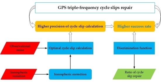26]. In contrast, GTCSR constructs a unified optimal model whose optimization objective has taken into account the influence of ionospheric delay, and minimizes the variance of the cycle slip combination at one time. Finally, GTCSR builds a cycle slip discrimination function to eliminate the adverse influence of large pseudorange errors on the fixation of the cycle slip combination. The epoch-difference, ionosphere-free, and geometry-free phase under GPS triple-frequency condition are designed as the discrimination function [28,29]. In this discrimination function, the pseudoranges are uninvolved; the ionospheric delay, geometric terms, and hardware biases are offset; and only the influence of cycle slips is retained. If the cycle slip values are correct, the absolute value of the discrimination function will be the smallest. Then, by sorting the discrimination values calculated by the candidates of the cycle slips, the reasonable cycle slip values are selected. Therefore, GTCSR is able to exclude the failure of cycle slip fixation caused by the significant bias in the cycle slip combination due to the large pseudorange error. In subsequent parts of this paper, the mathematical model of GTCSR is described. This is followed by an explanation of the testing strategies and conditions, and the experimental results are presented and analyzed. Finally, an in-depth discussion is carried out, and some beneficial conclusions are summarized.

2. Materials and Methods

The CSR method was established as follows. First, the mathematic model of calculating the cycle slip combination was built by correcting the ionospheric variation. Second, with the target to achieve the minimized variance of the cycle slip combination after correcting the ionospheric variation, the coefficients of the GPS triple-frequency combinations were supplied. Finally, a discrimination function was designed with the ionosphere-free and geometry-free phase, and the interference from the pseudorange error on CSR was excluded.

2.1. Ionospheric Variation Correction

If no cycle slip is contained in the epoch-difference phases, the ionospheric variation can be treated as the first-order difference of ionospheric delay [31,32], calculated with the epoch-difference phases as:

$$\Delta {\mathrm{iono}}_{1,\mathrm{k}}^{}=(\frac{\Delta {\varphi }_1^{}{\lambda }_1^{}-\Delta {\varphi }_2^{}{\lambda }_2^{}}{1-{\mathrm{f}}_1^2/{\mathrm{f}}_2^2}+\frac{\Delta {\varphi }_1^{}{\lambda }_1^{}-\Delta {\varphi }_3^{}{\lambda }_3^{}}{1-{\mathrm{f}}_1^2/{\mathrm{f}}_3^2})/2$$

(1)

where $\Delta$ is the epoch-difference operator on the adjacent epochs; $\Delta {\mathrm{iono}}_{1,\mathrm{k}}^{}$ is the ionospheric variation on carrier L1 at epoch k; $f_j^{}$ (j = 1,2,3) are the original frequencies on the GPS carriers of L1, L2, and L5, respectively; $\Delta {\varphi }_j^{}$ represents the epoch-difference phase on the frequency $f_j^{}$; and ${\lambda }_j^{}$ is the wavelength. If the triple-frequency phases are treated as independent on different frequencies and epochs, the variance of $\Delta {\mathrm{iono}}_{1,\mathrm{k}}^{}$ can be deduced as:

$${\delta }_{1,\Delta \mathrm{iono}}^2=(\frac{{\delta }_{\Delta {\varphi }_1^{}}^2{\lambda }_1^2+{\delta }_{\Delta {\varphi }_2^{}}^2{\lambda }_2^2}{(1-{\mathrm{f}}_1^2/{\mathrm{f}}_2^2{)}_{}^2}+\frac{{\delta }_{\Delta {\varphi }_1^{}}^2{\lambda }_1^2+{\delta }_{\Delta {\varphi }_3^{}}^2{\lambda }_3^2}{(1-{\mathrm{f}}_1^2/{\mathrm{f}}_3^2{)}_{}^2})/4$$

(2)

where ${\sigma }_{1,\Delta \mathrm{iono}}^{}$ is the standard deviation (STD) of $\Delta {\mathrm{iono}}_{1,k}^{}$ with the unit of m; and ${\sigma }_{\Delta {\varphi }_j^{}}^{}$ is the STD of $\Delta {\varphi }_j^{}$. If the STD of GPS phase ${\sigma }_{{\varphi }_j}^{}$ is 0.01 cycles, then ${\sigma }_{\Delta {\varphi }_j^{}}^2$= 0.0002 $cycl{e}_{}^2$ [33,34].

Furthermore, the second-order difference of ionospheric delay can be designed to investigate the characteristics of the ionospheric variation [10,20,24], and is expressed as:

$$\Delta \Delta {\mathrm{iono}}_{1,\mathrm{k}}^{}=\Delta {\mathrm{iono}}_{1,\mathrm{k}}^{}-\Delta {\mathrm{iono}}_{1,\mathrm{k}-1}^{}$$

(3)

The traditional CSD method with GF has been widely used in various GNSS data processing software. This method assumes a precondition that the first-order difference of ionospheric delay approaches 0. In this work, a more reasonable precondition is premised that the second-order difference of ionospheric delay approaches 0 [10,20,24]. Accordingly, the ionospheric variation calculated from the previous epoch is adopted to correct the ionospheric variation at the current epoch. The ionospheric variation can be gotten from the epoch-difference phases at the previous epoch. The preprocessing is implemented to find the first epoch without the cycle slip by using the CSD with GF (GFCSD). Then, we can start from the first epoch without the cycle slip to correct the ionospheric variation, and a lower ionospheric effect on CSR methods can be achieved.

2.2. Optimization of Cycle Slip Combination

The instrumental bias and multipath effect between adjacent epochs are regarded as constant over a short time interval [35,36,37]. After correcting the ionospheric variation, the cycle slip combination can be calculated with the combinations of triple-frequency phases and pseudoranges by:

$$\Delta N_{\mathrm{c}}^{}=\frac{\Delta p_c^{}}{{\lambda }_c^{}}-\Delta {\varphi }_c^{}-\Delta {\mathrm{iono}}_c^{}$$

(4)

where $\Delta N_c^{}={\displaystyle \sum _{j=1}^3{m}_j^{}}\Delta N_j^{}$ is the cycle slip combination; $m_j^{}$(j = 1,2,3) are the coefficients in the phase combination; $\Delta N_j^{}$ is the original cycle slip; ${\varphi }_c^{}={\displaystyle \sum _{j=1}^3{m}_j^{}}{\varphi }_j^{}$ is the phase combination; c is the velocity of light; ${\lambda }_c^{}=c/({\displaystyle \sum _{j=1}^3{m}_j^{}}{f}_j^{})$ represents the wavelength of ${\varphi }_c^{}$; $n_j^{}$(j = 1,2,3) are the coefficients in the pseudorange combination; $p_j^{}$ represents the pseudorange on the frequency $f_j^{}$; $p_c^{}={\displaystyle \sum _{j=1}^3{n}_j^{}}{p}_j^{}$ is the pseudorange combination; $ISF{C}_c={\displaystyle \sum _{j=1}^3{m}_j^{}}\frac{f_1^2}{{\lambda }_j^{}{f}_j^2}$ (wrt: L1, unit: cycle) is the ionospheric scaling factor (ISF) in ${\varphi }_c$; $ISF{P}_c={\displaystyle \sum _{j=1}^3{n}_j^{}}\frac{f_1^2}{f_j^2}$ (wrt: L1, unit: m) is the ISF in $p_c$; $IS{F}_c=ISF{\mathrm{C}}_c+ISF{P}_c/{\lambda }_c^{}$ (wrt: L1, unit: cycle) is the ISF in $N_c^{}$; $\Delta {\mathrm{iono}}_1^{}$(wrt: L1, unit: m) is the ionospheric variation on L1; so the ionospheric correction in $\Delta N_c^{}$ is $\Delta {\mathrm{iono}}_c^{}=\Delta {\mathrm{iono}}_1^{}IS{F}_c$.

The stochastic model of GNSS triple-frequency measurements is governed by both the internal errors of the receivers and external errors at the sites [38]. Different receivers or sites may result in distinct variances and covariance in the GNSS measurements. Considering the feasibility of optimization implementation and the wide reference of optimization results, the optimization on the multi-frequency combination usually takes the measurements on different frequencies and epochs to be independent. Therefore, the variance of $\Delta N_c^{}$ in (4) is presented as:

$${\sigma }_{\Delta N_c^{}}^2=\frac{2{\sigma }_{p_c^{}}^2}{{\lambda }_c^2}+2{\sigma }_{{\varphi }_c^{}}^2+{\sigma }_{c,\Delta iono}^2$$

(5)

where ${\sigma }_{{\varphi }_c}^{}=\sqrt{{\displaystyle \sum _{j=1}^3{\sigma }_{{\varphi }_{{}_j}^{}}^2}{m}_j^2}$ is the STD of ${\varphi }_c^{}$, and the unit of ${\sigma }_{{\varphi }_c}^{}$ is the cycle; ${\sigma }_{p_j}^{}$ is the STD of the GPS pseudorange; ${\sigma }_{P_c^{}}^{}=\sqrt{{\displaystyle \sum _{j=1}^3{\sigma }_{p_{{}_j}^{}}^2}{n}_j^2}$ is the STD of $p_c^{}$, and the unit of ${\sigma }_{p_c}^{}$ is meters. ${\sigma }_{1,\Delta iono}^{}$ is the STD of ionospheric variation correction on the L1 with the unit of m; ${\sigma }_{c,\varphi ,\Delta iono}^{}=\sqrt{{\displaystyle \sum _{j=1}^3(}\frac{{\sigma }_{1,\Delta iono}^{}{m}_j^{}{f}_1^2}{{\lambda }_j^{}{f}_j^2}{)}_{}^2}$ is the STD of ionospheric variation correction on the ${\varphi }_c^{}$, with the unit of cycle; and ${\sigma }_{c,p,\Delta iono}^{}=\sqrt{{\displaystyle \sum _{j=1}^3(\frac{{\sigma }_{1,\Delta iono}^{}{n}_j^{}{f}_1^2}{f_j^2}}{)}_{}^2}$ is the STD of ionospheric variation correction on the $p_c^{}$ with the unit of m. ${\sigma }_{c,\Delta iono}^{}=\sqrt{{\sigma }_{c,\varphi ,\Delta iono}^2+{\sigma }_{c,p,\Delta iono}^2/{\lambda }_c^2}$ is the STD of ionospheric variation correction on the cycle slip combination, with the unit of cycle.

As shown in (5), the variance of cycle slip combination is manipulated by the wavelength, the variances of phase and pseudorange, and the ionospheric correction noise. In nature, Equation (5) demonstrates that the longer the wavelength, the smaller the variances of phase combination and pseudorange combination, and the lower the residual effect after the ionospheric correction, which are beneficial to the smaller variance of the cycle slip combination. Thereby, this principle should be exerted to search the optimal coefficients in the combination of GPS triple-frequency phases and pseudoranges.

In order to achieve a higher precision of cycle slip combination, an optimal function is established to minimize the variance of the cycle slip combination as:

$$\min ({\sigma }_{\Delta N_{\mathrm{c}}^{}}^2)$$

(6)

with a geometry-free constraint:

$${\displaystyle \sum _{j=1}^3\frac{{\lambda }_c^{}}{{\lambda }_j^{}}{m}_j^{}}-{\displaystyle \sum _{j=1}^3{n}_j^{}}=0$$

(7)

A unified optimization model is formed with the target function of (6) by adding the constraint condition of (7). As a simple and useful way, the traversal search method can be employed to solve the optimization model. Consequently, three combinations are searched for the cycle slip combination, and the coefficients of the phase combinations should be linearly independent, so as to be utilized to transform the cycle slip combinations to the original cycle slips.

Results of the optimization model for the optimal calculation of GPS triple-frequency cycle slip combinations are listed.

Table 1. The optimized phase combinations of triple-frequency global position system (GPS).

${\mathit{\varphi }}_{7,\mathit{i}}$	${\mathit{m}}_{\mathit{i},\mathit{j}}^{}$	${\mathit{\lambda }}_{7,\mathit{i}}^{}\left(\mathbf{m}\right)$	${\mathit{\sigma }}_{{\mathit{\varphi }}_{7,\mathit{i}}}^{}\left(\mathbf{Cycle}\right)$	$\mathit{I}\mathit{S}\mathit{F}{\mathit{C}}_{7,\mathit{i}}(\mathbf{wrt}:\mathbf{L}1,\mathbf{Cycle})$
${\varphi }_{7,1}$	0,1,−1	5.861	0.0141	0.2932
${\varphi }_{7,2}$	−3,1,3	9.768	0.0436	−2.3686
${\varphi }_{7,3}$	4,−8,3	29.305	0.0943	13.8725

exhibits three optimized phase combinations, and

Table 2. The optimized pseudorange combinations and cycle slip combinations of triple-frequency GPS.

${\mathit{p}}_{7,\mathit{i}}$	${\mathit{n}}_{\mathit{i},\mathit{j}}^{}$	${\mathit{\sigma }}_{{\mathit{p}}_{7,\mathit{i}}}^{}\left(\mathbf{m}\right)$	$\mathit{I}\mathit{S}\mathit{F}{\mathit{P}}_{7,\mathit{i}}(\mathbf{wrt}:\mathbf{L}1,\mathbf{m})$	$\mathit{I}\mathit{S}{\mathit{F}}_{7,\mathit{i}}(\mathbf{wrt}:\mathbf{L}1,\mathbf{Cycle})$	${\mathit{\sigma }}_{\mathbf{\Delta }{\mathit{N}}_{7,\mathit{i}}}^{}\left(\mathbf{Cycle}\right)$
$p_{7,1}$	0,0.5106,0.4894	0.212	1.7219	0	0.0550
$p_{7,2}$	0.4,0.3,0.3	0.175	1.0280	12.2370	0.0858
$p_{7,3}$	0.3,0.3,0.4	0.175	1.5114	−11.7684	0.1434

shows three optimized pseudorange combinations. In brief, $m_{i,j}^{}$ (i = 1,2,3; j = 1,2,3) are the coefficients of phase combinations; ${\varphi }_{7,i}={\displaystyle \sum _{j=1}^3{\mathrm{m}}_{i,j}^{}}{\varphi }_j^{}$ (i = 1,2,3) are the optimized phase combinations; $n_{i,j}^{}$ (i = 1,2,3; j = 1,2,3) are the coefficients of pseudorange combinations; and $p_{7,i}={\displaystyle \sum _{j=1}^3{n}_{i,j}^{}}{p}_j^{}$ (i = 1,2,3) are the optimized pseudorange combinations.

With respect to ${\varphi }_{7,i}$ in Table 1, ${\lambda }_{7,i}^{}=c/({\displaystyle \sum _{j=1}^3{m}_{i,j}^{}}{f}_j^{})$ is the wavelength; ${\sigma }_{{\varphi }_{7,i}}^{}$ is the STD of ${\varphi }_{7,i}$; $N_{7,i}={\displaystyle \sum _{j=1}^3{\mathrm{m}}_{i,j}^{}}{N}_j^{}$ is the ambiguity combination; and $ISF{C}_{7,i}$ (wrt: L1, unit: cycle) is the ISF in ${\varphi }_{7,i}$. With respect to $p_{7,i}$ in Table 2, ${\sigma }_{p_{7,i}}^{}$ is the STD of $p_{7,i}$, and $ISF{P}_{7,i}$ (wrt: L1, unit: m) is the ISF in $p_{7,i}$. Finally, $IS{F}_{7,i}=ISF{\mathrm{C}}_{7,i}+ISF{P}_{7,i}/{\lambda }_{7,i}^{}$ (wrt:L1, unit: cycle) is the ISF in $\Delta N_{7,i}^{}$, and ${\sigma }_{\Delta N_{7,i}}^{}$ is the STD of $\Delta N_{7,i}^{}$.

2.3. Cycle Slip Solution

After correcting the ionospheric variation with the observed values at the precious epochs, the phase combinations and corresponding pseudorange combinations can be employed to calculate the cycle slip combinations as:

$$\Delta N_{7,i}^{}=\frac{\Delta p_{7,i}^{}}{{\lambda }_{7,i}^{}}-\Delta {\varphi }_{7,i}^{}-IS{F}_{7,i}\Delta {\mathrm{iono}}_{1,k-1}^{}$$

(8)

Then, the floats of $\Delta N_{7,i}^{}$ and their covariance matrix are obtained.

At first sight, the simple rounding can obtain the integer value of the floating value of $\Delta N_{7,i}^{}$ from Equation (8). Nevertheless, if the float of $\Delta N_{7,i}^{}$ has been biased by the large pseudorange error, more candidates of the cycle slip combinations need to be searched, and the final cycle slips should be discriminated from the candidates. Since LAMBDA provides an efficient integer search service, it is suggested to search the candidates of $\Delta N_{7,i}^{}$ via LAMBDA with the floating estimates and covariance matrix of $\Delta N_{7,i}^{}$ as the inputs. From the integers of $\Delta N_{7,i}^{}$, cycle slips on the original carriers $\Delta N_j$ (j = 1,2,3) can be easily transformed by:

$$\left[\begin{array}{c}\Delta N_1\\ \Delta N_2\\ \Delta N_3\end{array}\right]={\left[\begin{array}{ccc}0& 1& -1\\ -3& 1& 3\\ 4& -8& 3\end{array}\right]}_{}^{-1}\left[\begin{array}{c}\Delta N_{7,1}\\ \Delta N_{7,2}\\ \Delta N_{7,3}\end{array}\right]={\left[\begin{array}{ccc}27& 5& 4\\ 21& 4& 3\\ 20& 4& 3\end{array}\right]}_{}^{}\left[\begin{array}{c}\Delta N_{7,1}\\ \Delta N_{7,2}\\ \Delta N_{7,3}\end{array}\right]$$

(9)

This transformation demonstrates that the combination matrix consisted of coefficients $m_{i,j}^{}$(i = 1,2,3; j = 1,2,3), which are all integers, and vice versa, all elements of the inverse of the combination matrix are also integers.

2.4. Cycle Slip Discrimination against the Influence of the Pseudorange Error

The constituents can be carefully analyzed in the cycle slip combination from (8). Since the pseudoranges are involved in the calculation of the cycle slip combination, a large pseudorange error would disturb the normal calculation of the cycle slip combination. Unfortunately, large, even gross errors, are more likely to emerge in the pseudorange observations. If gross errors exist in the pseudorange, then a significant bias may result in the calculated float of the cycle slip combination.

In order to search the integer value of the cycle slip combination, LAMBDA was employed with the inputs of floats of the cycle slip combination and their covariance matrix. Then, the integers closest to the inputted floats under the statistical space represented by the covariance matrix are supplied by LAMBDA. Additionally, several candidate integers are provided. In the condition of the input floats without significant bias, the user can correctly apply LAMBDA. However, if a large bias exists in the float of the cycle slip combination, then the user has inputted a biased reference value to search the nearest integer. In this situation, the actual true integer may be distributed in the candidate values. Thereby, reasonable discrimination is required to eliminate the interference of a larger pseudorange error on the cycle slip determination and select the correct integer of the cycle slip combination from the candidates.

In terms of merely including the original epoch-difference phases, a special phase without geometric elements and ionospheric delay is built as:

$$\Delta L_8=\frac{f_1^2(\Delta {\varphi }_1+\Delta N_1){\lambda }_1-f_2^2(\Delta {\varphi }_2+\Delta N_2){\lambda }_2}{f_1^2-f_2^2}-\frac{f_1^2(\Delta {\varphi }_1+\Delta N_1){\lambda }_1-f_3^2(\Delta {\varphi }_3+\Delta N_3){\lambda }_3}{f_1^2-f_3^2}$$

(10)

where $\Delta L_8^{}$ is the ionosphere-free and geometry-free phase (IFGF) after the epoch-difference operation, and the geometry-free and ionosphere-free characteristics are an inspiring advantage [39].

Obviously, the ionospheric delay, geometric distance, clock error, orbit error, tropospheric delay, earth rotation effect, and relativity effect are cancelled in $\Delta L_8^{}$, and the smooth bias and multipath error are mitigated by the epoch-difference operation between adjacent epochs, then the $\Delta L_8^{}$ calculated with the correct cycle slips should approximate 0:

$$\Delta L_8^{}\to 0$$

(11)

LAMBDA has provided several candidates $\Delta {\mathrm{N}}_{7,i}(n)$, where n is the index number of the candidate values of cycle slip combinations. Using (9), the cycle slip combination $\Delta {\mathrm{N}}_{7,i}(n)$ can be transformed to the original cycle slip $\Delta N_{\mathrm{j}}^{}\left(n\right)$. Then, $\Delta L_8^{}(n)$ is obtained from the original phase $\Delta {\varphi }_{\mathrm{j}}$ and $\Delta N_{\mathrm{j}}^{}\left(n\right)$. According to (11), the epoch difference of IFGF repaired by the correct cycle slip approaches zero. Therefore, a discrimination function for selecting the minimized absolute values of $\Delta L_8^{}(n)$ is expressed as:

$$\min (\left|\Delta L_8^{}(\mathrm{n})\right|)$$

(12)

Following this guideline, the absolute values of $\Delta L_8^{}(n)$ calculated by the cycle slip candidates are sorted. As a result, the cycle slip values leading to the minimum of the absolute $\Delta L_8^{}$ are proposed by the discrimination function as the final cycle slip. In order to clarify the steps of GTCSR implementation, the process flow diagram is provided in Figure 1.

3. Results

The tests selected the real data under the circumstances of the severely active ionosphere and the quiet ionosphere. The experimental conditions designed the pseudoranges with large errors and the phases with small and special cycle slips. Then, various compared methods were implemented to validate the improvements made by this study. The compared results were analyzed as follows. First, after describing the testing data, the tests schemed the representative experiments and listed the conditions of the compared methods. Second, the actual correction precision of the ionospheric variation was examined. Third, the tests compared the performances of CSR before and after correcting the ionospheric variation. Fourth, the CSR comparisons were conducted with the real data, adding large errors on the actual pseudoranges epoch by epoch. Fifth, the small cycle slips and special cycle slips were utilized to evaluate the validity of different CSR methods. Finally, the tests investigated the success rates of different methods from all observable GPS triple-frequency satellites.

3.1. Test Description

Some compared tests were carried out to evaluate the performance of GTCSR. Three stations at various sites with different receivers and antenna types were selected and are listed in

Table 3. The information of the receivers and antennas.

Station name	Latitude	Receiver	Antenna
CUT0	−32.00	TRIMBLE NETR9	TRM59800.00
HKFN	22.49	LEICA GRX1200	LEIAT504
HKKT	22.36	LEICA GR25	LEIAR25.R4

. The CSR tests were conducted in two typical ionospheric circumstances. The one was the active ionosphere with severe variation under the 7-level geomagnetic storm that started from UTC 2016/05/08 00:00:00. The other was the quiet ionosphere that started from UTC 2016/05/10 00:00:00. The observation data were collected from the CUT0 station and the network of the Hong Kong Geodetic Survey Service with an interval of 30 s and the cutoff elevation of 10 degrees. All observable GPS triple-frequency satellites were included in the tests, and the statistical results are listed in the following section. In particular, considering the limitation of the paper length, only the results of satellites 10 and 25 during the geomagnetic storm were explicitly compared and exhibited.

The comparative schemes were arranged in

Table 4. The comparison of the different testing methods.

Compared Methods.	MW Cycle Slip Combination	Optimized Cycle Slip Combination	Correction the Ionospheric Variation	Selection with the Discrimination Function
GTCSR (Proposed)		✓	✓	✓
WICSR (Conventional)		✓
CTCSR (Conventional)		✓	✓
HMWCSD (Conventional)	✓

as follows. Scheme 1, the GTCSR developed in this study was tested, where the $\Delta N_{7,i}$(i = 1,2,3), after correcting the ionospheric variation, and the discrimination function (12) were employed to determine the cycle slip. Scheme 2, a method of CSR without ionospheric correction (WICSR) was used, where the ionospheric variations over the observed interval were treated as zero, and $\Delta N_{7,i}$(i=1,2,3) before ionospheric correction was directly used to fix the cycle slip. Scheme 3, a conventional triple-frequency CSR method (CTCSR) was utilized, where only $\Delta N_{7,i}$(i = 1,2,3) after ionospheric correction was employed, so the CSR results before the selection with the discrimination function were provided. Scheme 4, a conventional CSD method with GPS triple-frequency HMWs (HMWCSD) was employed to detect the cycle slip.

The extreme testing conditions were specified. First, a period during the geomagnetic storm was selected to investigate the influences of ionospheric variation on CSR and CSD, and examine the precision of ionospheric correction. Second, a gross error of 2.5 m, covering 99.99% pseudorange noises with the STD of 0.3 m was appended on all real triple-frequency pseudoranges epoch by epoch to inspect the performance of GTCSR resisting the influence of large pseudorange error. Finally, small cycle slips of (1,0,0), and (1,1,0) were chosen to confirm the validity of GTCSR, since these are hard to detect and repair, and have been usually utilized to test the CSR results by most researchers. Meanwhile, a special cycle slip of (1,1,1) was chosen, since this cycle slip causes HMWCSD to be invalid; moreover, a special cycle slip of (154,120,115) was chosen, since this cycle slip leads GFCSD to be invalid.

3.2. Precision Analysis of Ionospheric Variation Correction

For the observations during a 7-level geomagnetic storm at a low latitude region with an interval of 30 s, the ionospheric variations on L1 with the unit of meters were calculated from the real GPS data. Figure 2 shows the sequence of the first-order ionospheric delays, which describes the variations of ionospheric delays. In particular, the correction residuals of the ionospheric variations are embodied by the second-order ionospheric delays and are shown in the bottom parts of Figure 2.

Figure 2 shows that the ionospheric variations were remarkable, and reached up to 0.05 m in the latter time. The mean of the ionospheric variation was about 0.035 m. This indicates that significant ionospheric effects are contained in the epoch-difference phases. Unfortunately, the ionospheric effect will be magnified 12 times in the calculation of the cycle slip combination. Thereby, the variation of ionospheric delay must be corrected, otherwise, a striking bias will be produced in the calculation of the cycle slip combination.

The correction performance of ionospheric variation can be examined from the second-order difference of ionospheric delay. For the same data with an interval of 30 s, the mean of the second-order differences of ionospheric delays was about 0.00028 m. This indicates that, $\Delta \Delta {\mathrm{iono}}_{1,\mathrm{k}}^{}\to 0$, the ionospheric variation at the previous epoch $\Delta {\mathrm{iono}}_{1,\mathrm{k}-1}^{}$ can be employed to correct that of at the current epoch $\Delta {\mathrm{iono}}_{1,\mathrm{k}}^{}$.

3.3. Comparison of Cycle Slip Repair (CSR) Results under the Environment of Severe Ionospheric Variation

The period during the geomagnetic storm was selected to conducted the CSR tests. The test data experienced the environment with a severe ionospheric variation. The CSR performances were carefully compared with different CSR methods. GTCSR completed the correction of ionospheric variation, but WICSR was absent from correcting the ionospheric variation. Figure 3 shows the cycle slip combinations of GTCSR and WICSR, and the CSR results of GTCSR and WICSR are exhibited in Figure 4.

For the continuous phases, if $\left|\Delta {\mathrm{N}}_{7,i}\right|$ (i = 1,2,3) is far less than 0.5, the cycle slip value can be easily fixed to 0 as the true integer; otherwise, if $\left|\Delta {\mathrm{N}}_{7,i}\right|$ is close to or even larger than 0.5, the cycle slip value may be brought to the incorrect integer, leading to a repair failure. Figure 3 exhibits that the absolute values of $\Delta {\mathrm{N}}_{7,2}$ and $\Delta {\mathrm{N}}_{7,3}$ gradually approached and exceeded 0.5 in WICSR after 1000 s. Furthermore, the ionospheric variation contained in WICSR can be analyzed from Figure 2. The first-order difference of ionospheric delay increased obviously. After 1000 s, the ionospheric variation became larger than 0.03 m on L1, and reached 0.05 m. According to the ionospheric scaling factors in Table 2, the effects of ionospheric variation on the calculation of cycle slip combinations would be magnified 11–12 times. In this situation, the effects of ionospheric variation on the $\Delta {\mathrm{N}}_{7,2}$ and $\Delta {\mathrm{N}}_{7,3}$ could reach up to 0.3–0.6 cycles. Consequently, the CSR results in Figure 4 demonstrates that many failures occurred in WICSR due to the ionospheric variation, significantly polluting the calculation of the cycle slip combination.

For the same data without the cycle slip, GTCSR corrected the ionospheric variation, and obtained the cycle slip combinations shown in Figure 3. Figure 3 exhibits that the means of $\Delta {\mathrm{N}}_{7,2}$ and $\Delta {\mathrm{N}}_{7,3}$ in GTCSR approximated 0. The absolute values of $\Delta {\mathrm{N}}_{7,2}$ and $\Delta {\mathrm{N}}_{7,3}$ in GTCSR were distinctly smaller than those in the WICSR. This demonstrates that the ionospheric variation was notably diminished by GTCSR. Therefore, GTCSR can support the correct calculation of the cycle slip combination. As a result, the CSR results in Figure 4 demonstrate that all results of the GTCSR were correct.

3.4. Comparison of CSR Results under the Condition of Large Pseudorange Error

The random noise and multipath error were included in the actual pseudoranges. In order to inspect the upper limit of GTCSR on resisting the abnormal errors on the actual pseudoranges, gross error was imposed on the real pseudoranges. As the precision of normal pseudorange was 0.3 m, the STD of the epoch-difference pseudorange was 0.424 m. In fact, under the probability of 99.99%, the errors with a STD of 0.424 can be covered in the range of [−2.5, 2.5]. Thus, 2.5 m can almost cover the epoch-difference pseudorange errors of 99.99%, and was taken for the threshold value of epoch-difference pseudorange errors. In the following test of CSR against the larger pseudorange errors, we will append gross errors of (2.5,2.5,2.5) m epoch by epoch on all epoch-difference pseudoranges of real triple-frequency data collected from CUT0 station over a strong geomagnetic storm day.

CTCSR adopted the directly fixed cycle slip value $\Delta N_j$ from (8) and (9). The $\left|\Delta L_8\right|$ was calculated with the $\Delta N_j$ from CTCSR before the selection with the discrimination function. GTCSR offered the final cycle slip value $\Delta N_j$ after the selection with the discrimination function, and calculated the corresponding value of $\left|\Delta L_8\right|$. Then, the ratio was obtained with the $\left|\Delta L_8\right|$ of CTCSR before selection, dividing that of GTCSR after selection. Ratio equal to 1 indicates that the outputs from CTCSR are not falsely affected by the pseudorange error, while a ratio of larger than 1 declares that the outputs from CTCSR have been dramatically polluted by the pseudorange error.

The phases without the cycle slip and the epoch-difference pseudoranges adding a gross error of 2.5 m were employed to compare the performances of HMWCSD, GTCSR, and CTCSR. The cycle slip combinations of HMWCSD are exhibited in Figure 5. The results of CTCSR and GTCSR as well as the ratio are shown in Figure 6. The cycle slip combinations of GTCSR are displayed in Figure 7.

Figure 5 shows that all values of HMW visibly exceeded the detection limits, and HMWCSD appeared to have misjudgments in the situation of the epoch-difference pseudoranges with gross errors of 2.5 m and the phases without cycle slips. Looking into the values of the HMW cycle slip combinations, the range of the absolute values was between 0.5–4, that is, far larger than the detection limits of HMWCSD because remarkable biases were brought from the large pseudorange errors to the calculated values of the HMW cycle slip combinations. In fact, there were no cycle slips, and all cycle slips of HMW should stay within the detection limits.

Figure 6 shows that some cycle slip values from the CTCSR deviated from the correct value of 0, and CTCSR had failures in the situation of the epoch-difference pseudoranges with gross errors of 2.5 m and the phases without the cycle slip. As a result, many cycle slips are falsely fixed because of the interference of the large pseudorange error. The results of GTCSR after selection in Figure 6 show that the cycle slip values of GTCSR consisted with the correct value of 0, and GTCSR remained reliable in situations of the epoch-difference pseudoranges with gross errors of 2.5 m and the phases without the cycle slip. As the disturbance of the pseudorange error was eliminated by the selection with the discrimination function, the cycle slip values were determined reliably and correctly. Even though some absolute values of the cycle slip combinations approached or exceeded 0.5, the correct values of the cycle slip could also be found from the candidates by the discrimination function.

The discrimination ability can be investigated in light of the discrimination values, where the discrimination value is the $\left|\Delta L_8\right|$ calculated by the candidates of cycle slips. Figure 6 also shows the ratio of discrimination values between CTCSR and GTCSR. When the cycle slip value from CTCSR before selection is wrong, the ratio increases dramatically; while when the output of CTCSR is correct, the ratio stays at 1. This demonstrates that if the correct cycle slip is found, the absolute value of epoch-difference IFGF should be the smallest one among the $\left|\Delta L_8\right|$ calculated by the cycle slip candidates.

Figure 7 shows the values of cycle slip combinations during the period of strong geomagnetic storm. Some absolute values of $\Delta {\mathrm{N}}_{7,1}$ were between 0.4–0.6. This is the reason that resulted in the CDCSR output of the incorrect cycle slips. As significant biases were brought in the calculated values of the cycle slip combinations due to the pseudoranges polluted by large errors, once the biases approached or exceeded 0.5, the repaired results of CTCSR were incorrect.

3.5. Comparison of CSR Results against the Small and Special Cycle Slips

GTCSR dealt with the phase data with small cycle slips of (1,0,0) and (1,1,0) epoch by epoch, and output the floats of cycle slip combinations and the integers of original cycle slips, as shown in Figure 8 and Figure 9. On the other hand, GTCSR, GFCSD, and HMWCSD dealt with the phase data with special cycle slips of (1,1,1) and (154,120,115) epoch by epoch. GTCSR provided the floats of cycle slip combinations and the integers of original cycle slips, as shown in Figure 10 and Figure 11. The bottom parts of Figure 8, Figure 9, Figure 10 and Figure 11 are the sequence of original cycle slip values outputted from GTCSR. When the results of GTCSR are correct, the original cycle slip values outputted from GTCSR should be consistent with the inserted known cycle slip values.

Results of GTCSR processing the phase data with cycle slips of (1,0,0), (1,1,0), (1,1,1), and (154,120,115) are shown in Figure 8, Figure 9, Figure 10 and Figure 11. Since the values of the cycle slip combinations after correcting the ionospheric variation were distributed from −5 to 4, GTCSR received remarkable responses from the small cycle slips and special cycle slips. This means that GTCSR is sensitive and effective to the aforementioned small or special cycle slips, and better identification of the small or special cycle slips was achieved by GTCSR. Furthermore, the integers of the original cycle slips provided by GTCSR were consistent with the known cycle slip values. This demonstrates that the cycle slip values were determined correctly by GTCSR. Therefore, GTCSR can reliably and correctly repair the small and special cycle slips.

In contrast, HMWCSD was invalid to cope with the phase data with cycle slips of (1,1,1). Causally, for any integers N, the special cycle slips (N,N,N) on the original phases are embodied as zero in the HMW. This means that HMWCSD was insensitive to the aforementioned special cycle slips (N,N,N). Meanwhile, GFCSD was unable to deal with the phase data with cycle slips of (154,120,115). In reality, the special cycle slips (154N,120N,115N) on the original phases are embodied as zero in the GFs of L1–L2 and L1–L5 pairs because there is a principle that $154\mathrm{N}{\lambda }_1^{}=120\mathrm{N}{\lambda }_2^{}=115\mathrm{N}{\lambda }_3^{}$.

3.6. Statistical Results of All Observable Triple-Frequency GPS Satellites from Different CSR Methods

In this section, the real data collected from three types of receivers at different sites were processed during the geomagnetic storm and the quiet ionosphere. GTCSR, CTCSR, WICSR, and HMWCSD were employed to process the real GPS triple-frequency data, and those of adding a gross error of 2.5 m on all epoch-difference pseudoranges epoch by epoch. The statistical results of all observable triple-frequency GPS satellites can be analyzed in light of the CSR and CSD success rates. The CSR success rate is the correctly repaired number dividing the total repaired number. The CSD success rate is the correctly detected number dividing the total detected number.

Table 5. The success rates of all observable triple-frequency GPS satellites’ cycle slip processing results.

Compared Methods	Real Data During the Geomagnetic Storm	Real Data Adding Gross Errors of 2.5 m to all Epoch-Difference Pseudoranges during the Geomagnetic Storm	Real Data During the Quiet Ionosphere	Real Data Adding Gross Errors of 2.5 m to All Epoch-Difference Pseudoranges during the Quiet Ionosphere
HMWCSD (Conventional)	90.80%	1.17%	90.44%	1.00%
WICSR (Conventional)	94.89%	72.55%	98.57%	78.03%
CTCSR (Conventional)	100.00%	85.33%	99.79%	84.17%
GTCSR (Proposed)	100.00%	100.00%	100.00%	99.14%

shows the CSR success rates of GTCSR, CTCSR, WICSR, and the CSD success rate of HMWCSD from all observable triple-frequency GPS satellites.

For the real GPS triple-frequency data during the geomagnetic storm, the statistical results in Table 5 show that the CSR success rate of GTCSR was higher than that of WICSR. Obviously, the severe ionospheric variation caused a serious interference on the calculation and fixation of the cycle slip combination. WICSR does not correct the ionospheric variation, and results in a 5% failure rate. On the other hand, the calculation of the MW cycle slip combination and the detection of HMWCSD are affected by pseudorange noise, and a 10% failure rate occurs. However, the results of the GTCSR are correct. This confirms that GTCSR is capable of effectively correcting the ionospheric variations and suppressing the influence of pseudorange noise.

In the situation of adding a gross error of 2.5 m on all epoch-difference pseudoranges during the strong geomagnetic storm, Table 5 exhibits that 15% of the CTCSR results were incorrect because the large pseudorange error dramatically polluted the calculation and fixation of the cycle slip combination. In particular, the detection results of HMWCSD were almost completely wrong and unusable. However, the GTCSR results remained correct. This indicates that the discrimination function has a powerful ability to identify the correct cycle slip values, and eliminates the influence of large pseudorange errors on the fixation of the cycle slip combination.

For the real GPS triple-frequency data during the quiet ionosphere, the statistical results in Table 5 show that the CSR success rates of WICSR were higher than those during the geomagnetic storm. Clearly, the quiet ionospheric variation is beneficial to calculating the cycle slip combination, especially in the case of WICSR. However, on this day with the quiet ionosphere, the noise levels in the pseudoranges were higher than on that day with the geomagnetic storm, since the CSD success rates of HMWCSD were lower than those during the geomagnetic storm. Accordingly, the CSR success rates of CTCSR and GTCSR were lower than those during the geomagnetic storm. However, the success rate of GTCSR was still higher than that of CTCSR in the situation of adding a gross error of 2.5 m on all epoch-difference pseudoranges during the quiet ionosphere.

4. Discussion

All testing schemes were completed under various representative conditions covered by the weather including strong geomagnetic storm, the region over the ionospheric active area, and the observations with large pseudorange errors. The improvements of GTCSR were validated and compared with the following views. First, the correction performance of the ionospheric variation was evaluated with the second-order differences of ionospheric delays. Second, the performance of GTCSR resisting the severe ionospheric variation was compared with the WICSR without correcting the ionospheric variation during the geomagnetic storm. Third, the improvement of the discrimination function against the influence of large pseudorange error was evaluated by the comparisons of GTCSR, CTCSR, and HMWCSD in the case of adding large errors on all epoch-difference pseudoranges epoch by epoch. Fourth, the validity of GTCSR against small and special cycle slips was compared with those of HMWCSD and GFCSD. Finally, the actual success rates of all observable GPS triple-frequency satellites were compared from the aforementioned methods and the higher success rates were achieved in GTCSR.

GTCSR provides a simple and effective method to correct the ionospheric variation, and this method is more feasible and practical than the multi-epoch fitting method. Since as less than two epochs of the data already fulfill the correction of the ionospheric variation, this method would reduce the complexity and uncertainty resulting from involving more epochs of data. The correction residuals can be examined from the second-order differences of ionospheric delays. The ratio between the mean of first-order differences and that of second-order differences is about 125. This fact demonstrates that the ionospheric variations were significantly mitigated after the correction, and those of the residuals were merely 1/125 of the uncorrected ionospheric variations.

GTCSR established a unified optimal model to achieve the integrated optimization on calculating the cycle slip combination for the triple-frequency GPS. The influence of ionospheric delay is not separately considered behind the existing optimizations of triple-frequency combination. In an improved way, GTCSR built a unified optimal model with an integrated objective to minimize the variance of the cycle slip combination by taking into account the influence of ionospheric delay. Consequently, GTCSR provided an optimal way to calculate the cycle slip combination. The STDs of the cycle slip combinations of GTCSR were (0.055, 0.086, 0.143) cycles, which are clearly lower than those of the published optimal cycle slip combinations (0.186, 0.103, 0.189) cycles. Meanwhile, the ISFs of GTCSR were (0, 12.237, −11.768), which were obviously smaller than those of the published optimal cycle slip combinations (24.525, −12.283, −11.770) [24].

GTCSR obtained the cycle slip combinations that are valid to repair the small and special cycle slips, since the matrix of the combination coefficients is invertible, and the inverse matrix is also an integer matrix. The relationship between the original cycle slips and the cycle slip combinations is an integer transformation. A set of cycle slip combinations can only be converted into a unique set of original cycle slips, and there is no other polysemous values. When the cycle slip combinations are (0,0,0), the converted original cycle slips have a unique set with values of (0,0,0). There are no other nonzero original cycle slip values corresponding to the cycle slip combinations (0,0,0). Therefore, GTCSR can identify and repair all cycle slip values. In actual tests, small cycle slips (1,0,0), (1,1,0) and special cycle slips (1,1,1) and (154,120,115) were tested, respectively, and the results of GTCSR were correct.

GTCSR established a discrimination function to resist the adverse pollution of the pseudorange error on the fixation of the cycle slip. As the calculation of the discrimination function $\left|\Delta L_8\right|$ does not involve the pseudoranges, the pseudorange error no longer interferes with the value of $\left|\Delta L_8\right|$ and the sorting with $\left|\Delta L_8\right|$. Then, the influence of the pseudorange error is excluded by the selection with the discrimination function in GTCSR. The correct candidate of the cycle slip leads to a decrease in the value of $\left|\Delta L_8\right|$, but the wrong candidates result in increasing the value of $\left|\Delta L_8\right|$. Therefore, the discrimination function of GTCSR is effective at eliminating the interference of the pseudorange error and ensure the reliability of CSR. Following this principle, the sorting is implemented according to the $\left|\Delta L_8\right|$ calculated by the cycle slip candidates, then the cycle slip values resulting in the minimum $\left|\Delta L_8\right|$ are selected as the proposal cycle slip. In fact, as long as the correct cycle slip is covered by the candidates, the discrimination function could find the correct one as the proposal output. Thus, with the help of the discrimination function, the cycle slips are determined correctly and reliably, and the influence of pseudorange errors on CSR is also refrained.

It should be stressed that, although the results of GTCSR were correct in the case of the original real data during the quiet ionosphere and the severe active ionosphere experienced a geomagnetic storm, GTCSR produced a few mistakes in the situation of the original real data adding the gross error of 2.5 m on all epoch-difference pseudoranges during the quiet ionosphere. The reason is that they occasionally confronted abnormal influences that were 2.5 m of gross errors merging with the actual large noises of pseudoranges in the satellites with the elevations lower than 15 degrees, and the correct values of the cycle slip combinations would not be covered by the candidates. At this moment, GTCSR would also encounter CSR failures.

Fortunately, GTCSR dispenses with many restrictions such as the quiet ionosphere, the least number of observable satellites, or even the precise ephemeris, and so on. Thereby, GTCSR is helpful to the GPS precise application with the phase data such as the precise positioning, precise orbits determination, and so on. However, it is hard for a single study to traverse all extreme conditions and the vast observation data. In the future, it is recommended that GTCSR is evaluated by more users with a mass of observation data under both static and kinetic environments.

5. Conclusions

Cycle slip detection (CSD) is a prerequisite step in the generation and precise applications of GPS precise products with the phase data. For the phase data interrupted by the cycle slips, cycle slip repair (CSR) can play an important role in reducing the situations of ambiguity initialization and ensuring continuous convergence. Unfortunately, the severe ionospheric variation and large pseudorange error are adverse factors impeding the performances of CSD and CSR. Nevertheless, the developing triple-frequency research may bring new opportunities of coping with the aforementioned disadvantages. As some improvements on resisting the severe ionospheric variation and large pseudorange error, a GPS triple-frequency cycle slips repair method (GTCSR) was developed as follows:

(1)

An effective strategy was provided to correct the ionospheric variation. We introduced a more reasonable and rigorous condition where the second-order difference of the ionospheric delay approached 0. Therefore, the variation of the ionospheric delay at the previous epoch could be utilized to correct that of the current epoch, and the amplified ionospheric variation in the cycle slip combination was corrected before the calculation of the cycle slip combination.

(2)

The influences from the residuals of ionospheric correction were minimized for the purpose of optimal cycle slip calculation. This is the difference from the usual triple-frequency optimizations mainly focusing on the observational noises. As a result, the smaller amplified effect of the ionospheric correction residual, the lower noises, and the longer wavelength were achieved simultaneously, and the optimized coefficients were supplied to the optimal calculation of cycle slip combination.

(3)

A discrimination function was established to eliminate the influence of large pseudorange error on CSR and improve the reliability of CSR. We designed the epoch-difference expression of the ionosphere-free and geometry-free phase (IFGF), which solely reserves the significant respondence to the cycle slip, and excluded the interferences from the pseudorange error and ionospheric delay. With the help of the discrimination function, CSR failure was refrained from the biased cycle slip combination due to the pseudorange error.

Consequently, the performance of GTCSR was examined from comparative tests and extreme testing conditions. In the background of severe ionospheric variation during a strong geomagnetic storm over the low latitude area, the results of the GTCSR were correct, but the CSR without correcting the ionospheric variation (WICSR) appeared as failures. In the condition of adding 2.5 m gross errors to the real epoch-difference pseudoranges on each epoch, the conventional CSR with triple-frequency optimized combinations (CTCSR) and the CSD with HMW combination (HMWCSD) showed many incorrect results, but the success rate of GTCSR was significantly higher than those of CTCSR and HMWCSD. Meanwhile, GTCSR could repair the special cycle slips of (1,1,1) and (154,120,115), which were undetectable to the HMWCSD and GFCSD, respectively. Then, the ability of resisting the interferences of severe ionospheric variation and large pseudorange error on CSR was achieved by GTCSR, and the advantages of GTCSR were also evaluated.