Article

TomoSAR 3D Reconstruction for Buildings Using Very Few Tracks of Observation: A Conditional Generative Adversarial Network Approach

1
Key Laboratory of Technology in Geo-Spatial Information Processing and Application System, Chinese Academy of Sciences, Beijing 100194, China
2
Aerospace Information Research Institute, Chinese Academy of Sciences, Beijing 100094, China
3
School of Electronic, Electrical and Communication Engineering, University of Chinese Academy of Sciences, Beijing 101408, China
*
Author to whom correspondence should be addressed.
Remote Sens. 2021, 13(24), 5055; https://doi.org/10.3390/rs13245055
Submission received: 24 September 2021 / Revised: 28 October 2021 / Accepted: 10 December 2021 / Published: 13 December 2021
(This article belongs to the Special Issue Monitoring Urban Areas with Satellite SAR Remote Sensing)

Abstract

:
SAR tomography (TomoSAR) is an important technology for three-dimensional (3D) reconstruction of buildings through multiple coherent SAR images. In order to obtain sufficient signal-to-noise ratio (SNR), typical TomoSAR applications often require dozens of scenes of SAR images. However, limited by time and cost, the available SAR images are often only 3–5 scenes in practice, which makes the traditional TomoSAR technique unable to produce satisfactory SNR and elevation resolution. To tackle this problem, the conditional generative adversarial network (CGAN) is proposed to improve the TomoSAR 3D reconstruction by learning the prior information of building. Moreover, the number of tracks required can be reduced to three. Firstly, a TomoSAR 3D super-resolution dataset is constructed using high-quality data from the airborne array and low-quality data obtained from a small amount of tracks sampled from all observations. Then, the CGAN model is trained to estimate the corresponding high-quality result from the low-quality input. Airborne data experiments prove that the reconstruction results are improved in areas with and without overlap, both qualitatively and quantitatively. Furthermore, the network pretrained on the airborne dataset is directly used to process the spaceborne dataset without any tuning, and generates satisfactory results, proving the effectiveness and robustness of our method. The comparative experiment with nonlocal algorithm also shows that the proposed method has better height estimation and higher time efficiency.

Graphical Abstract

1. Introduction

The capability of inverting the spatial distribution in the elevation direction in each SAR azimuth-range imaging unit through multiple coherent SAR images makes TomoSAR an important technique in 3D information reconstruction of target objects [1,2]. Generally, numerous coherent SAR images (more than 20) [3] are required to obtain sufficient 3D reconstruction results. However, under realistic situations, only 3–5 practical tracks are available because of the constraints of cost and time. According to previous research, the accuracy of elevation inversion is proportional to the number of observation orbits and SNR [4]. Therefore, the accuracy of elevation inversion will decrease severely, which degrades the height estimation of buildings and damages the 3D architectural structures. Appropriate methods are needed in TomoSAR research under the condition of very few tracks.
Estimating the number of scatterers and their corresponding elevation are the essential steps in a TomoSAR procedure. The more accurate the elevation inversion is, the more refined information of buildings will be reconstructed, such as the overall architectural structure and the plane surface. However, the large errors in the elevation inversion with very few tracks severely damage these potential characteristics. As shown in Figure 1, the surface of a building is not a plane anymore and cannot be conjectured from the damaged blue points, the overall structure of building becomes fuzzy, and the height of the building will be estimated incorrectly.
Some traditional research of TomoSAR 3D reconstruction for buildings using a few tracks have been carried out. In 2015, XiaoXiang Zhu et al. used six-track coherent data to conduct research on building height estimation [5]. The geometric structures of the target buildings are obtained through the public optical building structure database to calculate the contour lines of buildings in SAR images. Then, the joint sparse estimation of the points on the contour lines are used to obtain the heights of contour lines. In 2020, HongLiang Lu et al. obtained the contour lines of the building directly from the SAR image through the contour line extraction algorithm (CLE) rather than other public databases [6]. However, the above methods need to be carried out by obtaining the geometry structures of the buildings, which is inconvenient and complicated. In 2020, Yilei Shi et al. proposed the nonlocal algorithm to deal with the building height estimation task with 3–5 tracks [4]. This algorithm performs patch-wise weighted filtering on the interferometric images, which effectively increases the SNR and obtains large-scale urban building 3D reconstruction results. However, the track configuration is specially set, so that the equivalent baseline length is long enough to maintain the elevation resolution. There is no research about the decrease of elevation resolution caused by the reduction of equivalent baseline length. In general, these studies lack automatic learning of the architectural structural characteristics and high-dimensional features of building.
There are also some studies on SAR 3D imaging using deep learning algorithms, which can automatically learn high-dimensional features of targets from data. In 2019, Siyan Zhou et al. proposed a deep fully connected network to denoise the 3D point cloud data of a single independent building to obtain a relatively flat surface [7]; however, this method cannot handle buildings with overlap and finds it hard to process the point cloud data of a large-scale scene. In 2021, Shihong Wang et al. proposed a 3D autoencoder network to filter the low-resolution 3D voxel data generated from three-track circular SAR data to approach the high-resolution results of all tracks [8]. However, this method requires a lot of computation and memory resources to process 3D voxel data, which is of low efficiency. In general, the deep learning algorithm has indeed brought new ideas into the research of SAR 3D reconstruction, enlightening the potential of deep learning algorithm in TomoSAR 3D information reconstruction for buildings with very few tracks.
The generation and development of generative adversarial network (GAN) has brought a major revolution into deep learning research. In 2014, Goodfellow first proposed the GAN principle and its network model [9], which gave rise to the research of generative networks. However, the native GAN is difficult to train and hard to converge. To deal with these problems, in 2015, Alec Radford et al. combined the GAN network structure with the deep convolutional network and proposed the Deep Convolutional GAN (DCGAN) [10]. The network structure of DCGAN solves the problems of unstable training and mode collapse, making it the main application of GAN network structures. Unfortunately, the DCGAN did not explain the problems of GAN theoretically. In order to fundamentally solve the problems, in 2017, Martin Arjovsky et al. analyzed the original loss function in depth and theoretically explained the problem of GAN nonconvergence, proposing WGAN [11]. Based on previous work, the GAN has important applications in image generation, style transfer, image synthesis, anti-spoofing, image deblurring, etc. [12,13,14,15,16]. However, the traditional GAN takes random noise as input. Generating a specific result based on the input content is called conditional GAN(CGAN), such as medical image segmentation and image deblurring tasks [17,18,19]. However, to our best knowledge, there is no research on the application of GAN in terms of SAR 3D reconstruction. This article will explore a method of applying a GAN network in SAR 3D imaging to generate refined and high-quality 3D results.
Traditional research of TomoSAR 3D reconstruction for buildings focuses on improving the solution of sparse equation by group sparsity based on contour lines or nonlocal algorithm increasing SNR. These methods are short of the automatic application of higher-dimensional features of buildings. In contrast, the deep learning algorithms show great potential in applying the high-dimensional features. The GAN network has a significant application in generating refined image results, which is very suitable for the task of 3D reconstruction of architectural targets. The code of our network is available here (https://gitee.com/WshongCola/cgan_for_few_tracks, accessed on 15 May 2021).
In summary, the key contributions of our work are as follows:
(1)
The Conditional generative adversarial network (CGAN) is originally applied to generate high-quality TomoSAR 3D reconstruction for buildings using very few tracks by learning the high-dimensional features of architectural structures.
(2)
Instead of directly processing large 3D data, the range-elevation 2D slices are processed to reduce network parameters and computational complexity, which makes it possible to deal with large-scale scenes. In order to solve the problem of possible misalignment among generations, the content loss between the input and generation is considered, so that the architectural structure can be reconstructed at the correct position.
(3)
The overlap of buildings in TomoSAR images makes buildings seem fused together and makes it hard to identify them from each other. The proposed method is able to distinguish the overlapped buildings correctly and estimate the heights of buildings. Compared with the widely used nonlocal algorithm, our method can estimate the height of buildings more accurately, and it is of higher time efficiency.

2. Materials and Methods

As shown in Figure 2, the proposed method is divided into two connected modules: data generation module and CGAN module.
Data Generation module:
Input: All coherent SAR images.
Output:
  • Low-quality slice set: The low-resolution and low-SNR range-elevation slices generated using three tracks by TomoSAR procedure.
  • High-quality slice set: The high-resolution and high-SNR range-elevation slices generated using all tracks.
The TomoSAR procedure is described in detail in Section 2.1.2
CGAN module:
Input data is the paired low-quality and high-quality slices generated by the data generation module. The network parameters are iteratively updated for learning the features between two pairs, obtaining the mapping relationship from low-quality slices to high-quality slices.

2.1. Data Generation Module

2.1.1. TomoSAR Principle

As shown in Figure 3, traditional synthetic aperture radars project the three-dimensional spatial distribution of scatterers along the elevation direction to the two-dimensional azimuth-range plane, which causes the elevation distribution of scatterers to be lost. TomoSAR expands the observing capabilities by multiple coherent tracks, making it possible to retrieve the elevation distribution information from coherent SAR images [20,21,22].
Assuming there are N tracks in total, according to previous research, the typical TomoSAR 3D imaging model can be formulated as follows [23]:
y n = s min s max σ ( s ) exp [ j 4 π λ R n ( s ) ] d s
In the above equation, y n represents the complex-value observation data of the nth antenna phase center (APC), expressed as the integral of the scatterer spatial distribution σ ( s ) along the elevation direction s. Taking a certain APC as the reference, the baseline length of the ith APC is b i . Discretizing the elevation range into M samples and considering noise, the continuous integral model can be approximated as
y = Φ · σ + n
where y is the complex-value observation data vector in each azimuth-range unit of corresponding APCs. Φ is the observation matrix, which bridges the observation vector and elevation distribution. The element of matrix is Φ i , j = exp ( j 4 π b i s j λ R ) , where s j is the jth elevation discretized resolution cell, and R is the distance between the scatterers and APC. Based on Equation (2), the elevation distribution σ ( s ) in each azimuth-range unit can be inverted from y .
According to the Fourier analysis principle [24], assuming the maximum baseline length is B, the Rayleigh resolution in the elevation direction is ρ s = λ R 2 B , and the observation matrix can be expressed as exp ( j 2 π ξ i s j ) , where ξ i = 2 b i 2 B is the spatial frequency. Equation (2) can be regarded as the Fourier transform of σ . The sampling interval of spatial frequency is Δ ξ = 2 Δ b λ R , where Δ b is the interval length between two neighboring APCs. Based on the theory of space–time analysis, the maximum unambiguity range of the elevation direction is s u a = λ R 2 Δ b . According to the above theoretical analysis and the research in [4], the less the number of available track is, the shorter the maximum baseline length will be, leading to a decrease in the elevation spatial resolution.
Based on the theory of linear algebra, when the number of samples M in the elevation direction is much larger than the practical number of coherent tracks, Equation (2) becomes an underdetermined equation with a nonunique solution space. The general solution is to use the compressed sensing (CS) method [25,26,27]. The objective function with the sparse constraint item is as follows:
σ ^ = arg min x { Φ · σ y 2 2 + λ σ 1 }
In the above equation, λ represents the sparse coefficient. The larger the value is, the sparser the solution will be. σ 1 is the sparse constraint item to limit the solution space.

2.1.2. TomoSAR Procedure

As shown in Figure 4, firstly, the azimuth-range units in different SAR images should be related to the same scatterers after registration [28]. Secondly, channel phase errors, which are caused by positioning or system errors, are compensated to focus the inversion results in the elevation direction. The minimum entropy method is applied to estimate the phase errors. Thirdly, the sparse recovery methods are used to estimate the elevation positions of scatterers in each azimuth-range unit. Finally, the coordinate system is transformed from radar system into geodetic system.

2.1.3. Data Generation

Figure 5 illustrates the procedure of data generation.
Paired super-resolution dataset: The paired dataset contains the low-quality and high-quality slice sets. Slices of different sets in the same azimuth position are paired to be input and corresponding ground truth.
Low-quality slice set: The low-quality slice set is composed of binarized 2D range-elevation slices generated using three adjacent tracks through algorithms in TomoSAR procedure, which is of low SNR and low elevation spatial resolution. The equivalent baseline length of three adjacent tracks is much shorter than that of full tracks, which will severely decrease the elevation resolution. This low-quality set is the input data of the network. The binary operation means that the value set is 1 if a scatterer is estimated in this position.
High-quality slice set: The high-quality slice set shares the same procedure as the low-quality set, but uses all SAR images to generate high-SNR and high-elevation spatial resolution data.
All slices are in radar coordinate system.

2.2. CGAN Module

The CGAN consists of two models, the generator and the discriminator, as shown in Figure 6. The generator produces a fake result as similar as possible to the high-quality ground truth based on the low-quality input. The role of the discriminator is to distinguish the fake result and the ground truth. Through iterative optimization, the generator needs to produce a result as similar as possible to make the discriminator believe it is the truth, and the discriminator needs to distinguish the fake result from ground truth as much as possible.

2.2.1. Generator

The generator network structure based on the autoencoder [19] is shown in Figure 7, which can be roughly divided into three main parts: downsampling compression, feature extraction, and upsampling reconstruction. In the downsampling compression part, four times downsampling is achieved through two convolution networks with step of two, and the feature dimension is expanded from 64 to 256, which is indicated by the number on the left side of blocks, such as n64. The feature extraction part digs out high-dimensional features from the downsampled data by stacking nine layers of deep convolution blocks. The upsampling reconstruction part uses two deconvolution (TransposedConv) layers with step of two to achieve four times upsampling and decrease the feature dimension to one.
In order to accelerate the convergence of the network, the generator adopts the residual network structure, which adds the input data straight into the output, learning the difference between the input and output. In addition, an InstanceNorm module has been applied to accelerate the network convergence by normalizing each channel in the convolution layers.

2.2.2. Discriminator

A Markovian discriminator [29] is applied in the proposed method, which is different from other discriminators that generate one real number based on the network input to indicate the probability that the input is truth. In contrast, the Markovian discriminator generates a matrix. Each element of the matrix represents the truth probability of a small area in the receptive field. Finally, the average of matrix is regraded as the probability that the entire picture is the truth. The discriminator structure is shown in Figure 8.
The discriminator network is composed of four convolutional layers, which contain convolution model, BatchNorm model, and LeakyReLU model in each layer, and the last layer is only a convolutional model with one filter to generate the truth possibility map. The BatchNorm model is used to accelerate the convergence of network and the LeakyReLU is used as activation function.

2.2.3. Loss Function

The total loss is formulated as follows:
L = L G A N + λ · L x
In Equation (4), the total loss is the sum of adversarial loss L G A N and content loss L x , which is balanced by parameter λ . The adversarial loss is formulated as follows:
L D G A N = E x P h i g h _ r e s [ D ( x ) ] + E z P l o w _ r e s [ D ( G ( z ) ) ]
L G G A N = E z P l o w _ r e s [ D ( G ( z ) ) ]
In Equation (5), the loss function of the discriminator is formulated as two parts. The first part is E x P h i g h _ r e s [ D ( x ) ] , x is sampled from the high- resolution dataset, and it is processed by the discriminator D ( ) . The second part is E z P l o w _ r e s [ D ( G ( z ) ) ] , where z is sampled from the high-resolution dataset correspondingly. The input data z is processed by the generator G ( ) to produce a fake result G ( z ) , then the fake result is processed by the discriminator D ( ) . The discriminator D ( ) will give a score to indicate the truth of input data. The higher the score, the more the judge believes that the data entered is true. Therefore, the discriminator tries to give high score to the high-res input and low score to the low-res input to minimize the loss function. In Equation (6), the generator tries to produce fake results similar to high-res input, so that the discriminator will give high score to the fake result.
In order to make the generated results relevant to the content of the input data, the content loss is applied. However, minimizing the L1 or L2 distance between the generated result and the ground truth in pixel-wise will lead to blurry artifacts in generated results. Therefore, in this paper, the feature extraction network is adopted to measure the distance in perceptual domain, which is expressed as follows:
L x = 1 W i , j H i , j x = 1 y = 1 ( ϕ i , j ( I G T ) x , y ϕ i , j ( G θ G ( I I N ) ) x , y ) 2
In Equation (7), ϕ i , j represents the result of the feature layer between the jth maximum pooling after the ith convolutional layer after activation. By constraining features in different levels, such as high semantic feature level and low detail level, the generated result will be refined and fit the ground truth much better.

3. Results and Discussion

3.1. Network Training

Data augmentation: Training of CGAN requires an amount of data. However, the number of slices of a building in a TomoSAR scene is insufficient; only hundreds of slices are available. The network will try to memorize these slices rather than learning the deep features. To solve this problem, the data augmentations, including random combination, flipping, and translation, are applied on the input slices. The application of random combination tries to simulate the condition of many buildings by placing slices of one isolated building at different azimuth positions together into one fabricated slice. Besides this, the additional noise is used to improve the robustness of network.
Training configurations: The network is trained on AMD Ryzen 5 2600 Six-Core CPU and 1 NVIDIA GeForce GTX 1080Ti GPU. The optimizer is Adam. In a total of 150 epochs, the learning rate in the first 100 epochs is 0.0001 and is linearly reduced to 0 in the last 50 epochs. According to GPU memory limitation, the input size is set as 1200 * 256, while the batchsize is 14. The network converges after 100 epochs in our experiments. The critic function of GAN is Wasserstein GAN with Gradient Penalty (wgan-gp) [11], which can solve the problem of gradient disappearance and explosion. The perceptual network named VGG19 [30] pretrained on ImageNet is adopted to calculate the difference between the feature maps of fake result and ground truth.

3.2. Airborne Dataset

The YunCheng airborne data is used in the experiment. The parameters are listed in Table 1.
There are nine buildings in Figure 9, which are indicated with rectangles and numbered in both the optical and intensity SAR images correspondingly. The buildings #1 and #2, marked with red color, are selected as training set, and the other buildings with white color are the testing set. Obviously, in the SAR image, three (#3, #4, #5) buildings are overlapped. Meanwhile, the four (#6, #7, #8, #9) buildings are nonoverlapped. Both the overlapped objects and nonoverlapped objects are indicated with white dotted rectangles. In order to explain the reconstruction results of overlapped and nonoverlapped objects more intuitively, two slices are selected at the positions of slice 1 and slice 2 in Figure 9b. Slice 1 is the elevation-range image of buildings #6, #7, #8, and #9, while slice 2 is the corresponding view of buildings #1, #2, #3, and #4. Building #5 shared the same characteristics as building #4 and is not listed here.
In Figure 10, the 3D height and strength distribution of both all-track and three-track TomoSAR results are shown. Figure 10b,d show the normalized strength distributions. Compared with the three-track result, the dominant scatterers mainly locate at the surface of buildings and the structures are much more refined. In Figure 10a,c, it is obvious that the quality of the three-track TomoSAR 3D result is much lower than that of the all-track TomoSAR. According to the previous analysis, it is proved that the three-track TomoSAR of low SNR and resolution will definitely introduce large errors in the elevation inversion, resulting in fuzzy architectural structures.
In order to explore the ability of the network in dealing with both overlapped and nonoverlapped situations, the total buildings are divided into two testing sets.
In this experiment, the configurations of nonlocal algorithm [31,32,33,34,35] are set as follows in Table 2, according to the recommendations in [32].

3.2.1. Nonoverlapped Buildings

Figure 11a,c are the height maps of all-track and three-track TomoSAR results of nonoverlapped buildings #6, #7, #8, and #9, while Figure 11b,d are normalized strength maps. Compared with all-track TomoSAR results, the results of three-track TomoSAR are much worse with lots of artifacts and outliers. Besides, there is inevitable powerful multipath scattering [36] marked with red circles that affects the structures. In addition, the heights of buildings are estimated and labeled with orange lines in strength maps.
In Figure 12, the results of nonlocal algorithm and proposed CGAN method are shown and compared. From the normalized strength maps in Figure 12b,d, the nonlocal algorithm can indeed remove the artifacts and outliers by increasing the SNR. However, there are still some artifacts and outliers remaining. In contrast, the results of the proposed CGAN method are of higher quality with fewer artifacts and outliers. Meanwhile, the multipath scattering marked by red circles is also well suppressed, which affected the structures in nonlocal results.

3.2.2. Overlapped Buildings

Figure 13a shows the height and strength maps of buildings #3 and #4 reconstructed using all and three tracks. In Figure 13a, the structures of two overlapped buildings can be clearly recognized. In Figure 13b, the dominant scatterers mainly locate at the surface of buildings. There is a large interval between two buildings. However, it is found in Figure 13c that the two buildings are difficult to distinguish from each other without obvious boundaries. The strength map in Figure 13d also shows that the scatterers of two buildings almost merge together, which severely damages the structures of two buildings.
In Figure 14, the results of the proposed CGAN method and nonlocal algorithm are shown. Figure 14a is the height map of nonlocal algorithm, and Figure 14d is the normalized strength map. The nonlocal algorithm can greatly distinguish between two overlapped buildings with an obvious interval in between. Meanwhile, Figure 14c,d are the results of proposed CGAN method. Similarly, the proposed method can also distinguish between two overlapped buildings with a large interval in between. However, it becomes worse when it comes to the height estimation of building #3. The height estimated by the nonlocal algorithm is severely different from that of the all-track results. In contrast, the height estimated by the proposed CGAN method is closer to that of the all-track results.
In Figure 15, it should be noted that although the nonlocal algorithm can effectively improve the overall 3D imaging quality, the structures of buildings are still blurry compared to CGAN results. In other words, the imaging results of the proposed CGAN method are much clearer, and it has stronger ability to suppress the artifacts, outliers, and multipath scattering.
The heights of buildings are mainly considered when building the 3D reconstruction task. Therefore, buildings #3, #4, #6, #7, #8, and #9 are estimated according to the strength maps by different methods. The results are as follows:
Table 3 is the comparison of building height estimations by different methods. Limited by the resolution and error of subjective judgment, the errors under 2 m are negligible. The main focus is on the height estimation results of building #3, #4, and #7, whose errors cannot be ignored. For building #3, there are large errors in the three-track and nonlocal estimations, compared to all-track result. It may be caused by the powerful multipath scattering under the condition of three tracks, which damages the roof structure of building. For building #4, it is difficult to judge the height because the interval between buildings #3 and #4 are too small to separate them. Furthermore, the roof of building #4 merges with the surface of building #3, which makes it harder to identify the roof. For building #7, it can be seen that both the three-track TomoSAR and the nonlocal algorithm estimated results have large errors. From the respective intensity distribution maps, it can be seen that the dominant influence is the multipath scattering of the nearby building, which damages the roof of the target building severely.
Table 4 compares the time consumption of the nonlocal algorithm and the proposed CGAN method in reconstructing the entire scene. The nonlocal algorithm is accelerated using the vector parallel acceleration calculation technique, which occupies lots of memory and consumes about 4 h. In contrast, the noniterative parallel calculation of the proposed CGAN network consumes about 10 s to process the entire scene. It is obvious that the proposed CGAN method has much higher time efficiency than the iterative nonlocal algorithm.

3.3. Spaceborne Dataset

We use the spaceborne dataset from TerraSAR-X in Barcelona to demonstrate the effectiveness and robustness of our method. The parameters are listed in Table 5. Figure 16 shows the optical image of target building and corresponding SAR intensity image.
In Figure 17, the 3D views of the CS method using all tracks and only three tracks are shown. While using only three tracks, the CS method introduces lots of outliers. On the contrary, the all-track reconstruction shows few outliers and refined building surface.
In Figure 18, the CS method is applied to reconstruct building surface using three and all tracks. While using three tracks, there are lots of outliers marked by orange circles, which has strong intensity. In contrast, there are fewer outliers in the all-track reconstruction result; however, the building surfaces of all results are not smooth.
In Figure 19, the comparison of reconstruction results of the nonlocal algorithm and the CGAN method while using only three tracks is shown. Generally, the nonlocal algorithm can compress the outliers. In contrast, the proposed CGAN method can not only greatly compress the outliers, but also generate refined building surface.
In order to estimate the effectiveness and robustness of the proposed CGAN method, we directly use the network trained on the airborne dataset to process the spaceborne dataset. Surprisingly, the pretrained network, without any tuning on the spaceborne dataset, also shows reasonable results.
The heights of buildings using several methods are labeled in strength maps using orange lines. There is no significant difference among these estimations, proving that the proposed CGAN method can correctly reconstruct the height of buildings in the spaceborne dataset.
In Figure 20, 3D views of the nonlocal algorithm and the proposed CGAN method are compared. There are many outliers in the results of the nonlocal algorithm using three tracks. However, compared with the CS method, it slightly compresses the outliers. In contrast, the number of outliers is significantly lower in the CGAN method. Furthermore, the surface of buildings generated by our method is smooth and refined.
Importantly, instead of tuning on the spaceborne dataset, the network directly uses the network pretrained on the airborne dataset to process the spaceborne dataset. In terms of results, the CGAN approach has also yielded satisfactory reconstruction results, which proves the effectiveness and robustness of our methodology.

4. Conclusions

In this article, we propose the CGAN model to generate satisfactory TomoSAR 3D reconstruction for buildings using three tracks.
Firstly, we introduced the principle of TomoSAR imaging and theoretically analyzed the consequences of using very few tracks. Secondly, we proposed the CGAN model and explained the network structures in detail. Besides this, we described the procedure of data generation to meet the requirement of a large amount of training data.
The experiments on the YunCheng airborne dataset and TerraSAR-X spaceborne dataset prove the capabilities of the proposed CGAN method in improving TomoSAR 3D reconstruction using three tracks in both quality and quantity. Furthermore, to explain the efficiency and effectiveness, we also compared it with the nonlocal algorithm used in previous research. The comparison results indicate that the proposed CGAN method can produce more refined structures of buildings and more accurate height estimation. Moreover, the nonlocal algorithm takes over 4 h to finish the entire scene. In contrast, the proposed method only takes around 10 s, proving the time efficiency of our method.
However, in this paper, only the features in the 2D elevation-range slice are considered because of the computation complexity. It is believed that the reconstruction results will be better with the features considered in all three dimensions (azimuth, range, elevation). Besides this, the training dataset is also limited because the TomoSAR data of buildings is hard to access and consumes lots of time to generate a super-resolution dataset. In the future, more work will be carried out to explore the application of 3D features in TomoSAR 3D reconstruction for buildings.

Author Contributions

Conceptualization, S.W., J.G., Y.Z., C.D. and Y.W.; Methodology, S.W.; Resources, J.G., Y.H., C.D. and Y.W.; Software, S.W.; Supervision, J.G., Yueting Zhang, Y.H., C.D. and Y.W.; Writing—original draft, S.W.; Writing—review & editing, J.G. and Yueting Zhang. All authors have read and agreed to the published version of the manuscript.

Funding

This research was funded by The National Natural Science Foundation of China grant number 61991421, 61991420.

Institutional Review Board Statement

Not applicable.

Informed Consent Statement

Not applicable.

Data Availability Statement

The spaceborne dataset used in this article is not publicly available, as it was purchased. A publicly available airborne dataset was analyzed in this study. This data can be found here: (http://radars.ie.ac.cn/web/data/getData?dataType=SARMV3D_en&pageType=en, accessed on 15 May 2021).

Conflicts of Interest

The authors declare no conflict of interest.

References

  1. Reigber, A.; Moreira, A. First Demonstration of Airborne SAR Tomography Using Multibaseline L-Band Data. IEEE Trans. Geosci. Remote Sens. 2000, 38, 2142–2152. [Google Scholar] [CrossRef]
  2. Frey, O.; Meier, E. Analyzing Tomographic SAR Data of a Forest With Respect to Frequency, Polarization, and Focusing Technique. IEEE Trans. Geosci. Remote Sens. 2011, 49, 3648–3659. [Google Scholar] [CrossRef] [Green Version]
  3. Zhu, X.X.; Bamler, R. Very High Resolution Spaceborne SAR Tomography in Urban Environment. IEEE Trans. Geosci. Remote Sens. 2010, 48, 4296–4308. [Google Scholar] [CrossRef] [Green Version]
  4. Shi, Y.; Bamler, R.; Wang, Y.; Zhu, X.X. SAR Tomography at the Limit: Building Height Reconstruction Using Only 3–5 TanDEM-X Bistatic Interferograms. IEEE Trans. Geosci. Remote Sens. 2020, 58, 8026–8037. [Google Scholar] [CrossRef]
  5. Zhu, X.X.; Ge, N.; Shahzad, M. Joint Sparsity in SAR Tomography for Urban Mapping. IEEE J. Sel. Top. Signal Process. 2015, 9, 1498–1509. [Google Scholar] [CrossRef] [Green Version]
  6. Lu, H.; Zhang, H.; Deng, Y.; Wang, J.; Yu, W. Building 3-D Reconstruction With a Small Data Stack Using SAR Tomography. IEEE J. Sel. Top. Appl. Earth Obs. Remote Sens. 2020, 13, 2461–2474. [Google Scholar] [CrossRef]
  7. Zhou, S.; Li, Y.; Zhang, F.; Chen, L.; Bu, X. Automatic Reconstruction of 3-D Building Structures for TomoSAR Using Neural Networks. In Proceedings of the 2019 IEEE International Conference on Signal, Information and Data Processing (ICSIDP), Chongqing, China, 11–13 December 2019; pp. 1–5. [Google Scholar] [CrossRef]
  8. Wang, S.; Guo, J.; Zhang, Y.; Hu, Y.; Ding, C.; Wu, Y. Single Target SAR 3D Reconstruction Based on Deep Learning. Sensors 2021, 21, 964. [Google Scholar] [CrossRef]
  9. Goodfellow, I.J.; Pouget-Abadie, J.; Mirza, M.; Xu, B.; Warde-Farley, D.; Ozair, S.; Courville, A.; Bengio, Y. Generative Adversarial Networks. arXiv 2014, arXiv:1406.2661. [Google Scholar] [CrossRef]
  10. Radford, A.; Metz, L.; Chintala, S. Unsupervised Representation Learning with Deep Convolutional Generative Adversarial Networks. arXiv 2015, arXiv:1511.06434. [Google Scholar]
  11. Gulrajani, I.; Ahmed, F.; Arjovsky, M.; Dumoulin, V.; Courville, A. Improved Training of Wasserstein GANs. arXiv 2017, arXiv:1704.00028. [Google Scholar]
  12. Karras, T.; Laine, S.; Aila, T. A Style-Based Generator Architecture for Generative Adversarial Networks. arXiv 2019, arXiv:1812.04948. [Google Scholar]
  13. Wang, W.; Huang, Q.; You, S.; Yang, C.; Neumann, U. Shape Inpainting Using 3D Generative Adversarial Network and Recurrent Convolutional Networks. arXiv 2017, arXiv:1711.06375. [Google Scholar]
  14. Zhang, H.; Xu, T.; Li, H.; Zhang, S.; Wang, X.; Huang, X.; Metaxas, D. StackGAN: Text to Photo-Realistic Image Synthesis with Stacked Generative Adversarial Networks. arXiv 2017, arXiv:1612.03242. [Google Scholar]
  15. Brock, A.; Donahue, J.; Simonyan, K. Large Scale GAN Training for High Fidelity Natural Image Synthesis. arXiv 2018, arXiv:1809.11096. [Google Scholar]
  16. Tolosana, R.; Vera-Rodriguez, R.; Fierrez, J.; Morales, A.; Ortega-Garcia, J. DeepFakes and Beyond: A Survey of Face Manipulation and Fake Detection. arXiv 2020, arXiv:2001.00179. [Google Scholar] [CrossRef]
  17. Wang, X.; Han, S.; Chen, Y.; Gao, D.; Vasconcelos, N. Volumetric Attention for 3D Medical Image Segmentation and Detection. arXiv 2004, arXiv:2004.01997. [Google Scholar]
  18. Yu, Q.; Xia, Y.; Xie, L.; Fishman, E.K.; Yuille, A.L. Thickened 2D Networks for Efficient 3D Medical Image Segmentation. arXiv 2019, arXiv:1904.01150. [Google Scholar]
  19. Kupyn, O.; Budzan, V.; Mykhailych, M.; Mishkin, D.; Matas, J. DeblurGAN: Blind Motion Deblurring Using Conditional Adversarial Networks. arXiv 2018, arXiv:1711.07064. [Google Scholar]
  20. Zhu, X.X.; Bamler, R. Super-Resolution of Sparse Reconstruction for Tomographic SAR Imaging—Demonstration with Real Data. In Proceedings of the EUSAR 2012 9th European Conference on Synthetic Aperture Radar, Nuremberg, Germany, 23–26 April 2012; pp. 215–218. [Google Scholar]
  21. Zhu, X.X.; Bamler, R. Sparse Reconstrcution Techniques for SAR Tomography. In Proceedings of the 2011 17th International Conference on Digital Signal Processing (DSP), Corfu, Greece, 13–15 June 2011; pp. 1–8. [Google Scholar] [CrossRef]
  22. Zhu, X.X.; Adam, N.; Bamler, R. Space-Borne High Resolution Tomographic Interferometry. In Proceedings of the 2009 IEEE International Geoscience and Remote Sensing Symposium, Cape Town, South Africa, 12–17 July 2009; Volume 4, pp. IV–869–IV–872. [Google Scholar] [CrossRef]
  23. Jiao, Z.; Ding, C.; Qiu, X.; Zhou, L.; Chen, L.; Han, D.; Guo, J. Urban 3D Imaging Using Airborne TomoSAR: Contextual Information-Based Approach in the Statistical Way. ISPRS J. Photogramm. Remote Sens. 2020, 170, 127–141. [Google Scholar] [CrossRef]
  24. Fornaro, G.; Lombardini, F.; Pauciullo, A.; Reale, D.; Viviani, F. Tomographic Processing of Interferometric SAR Data: Developments, Applications, and Future Research Perspectives. IEEE Signal Process. Mag. 2014, 31, 41–50. [Google Scholar] [CrossRef]
  25. Xiang, Z.X.; Bamler, R. Compressive Sensing for High Resolution Differential SAR Tomography-the SL1MMER Algorithm. In Proceedings of the 2010 IEEE International Geoscience and Remote Sensing Symposium, Honolulu, HI, USA, 20–30 July 2010; pp. 17–20. [Google Scholar] [CrossRef] [Green Version]
  26. Weiß, M.; Fornaro, G.; Reale, D. Multi Scatterer Detection within Tomographic SAR Using a Compressive Sensing Approach. In Proceedings of the 2015 3rd International Workshop on Compressed Sensing Theory and Its Applications to Radar, Sonar and Remote Sensing (CoSeRa), Pisa, Italy, 17–19 June 2015; pp. 11–15. [Google Scholar] [CrossRef]
  27. Lie-Chen, L.; Dao-Jing, L. Sparse Array SAR 3D Imaging for Continuous Scene Based on Compressed Sensing. J. Electron. Inf. Technol. 2014, 36, 2166. [Google Scholar] [CrossRef]
  28. Guizar-Sicairos, M.; Thurman, S.T.; Fienup, J.R. Efficient Subpixel Image Registration Algorithms. Opt. Lett. 2008, 33, 156–158. [Google Scholar] [CrossRef] [PubMed] [Green Version]
  29. Isola, P.; Zhu, J.Y.; Zhou, T.; Efros, A.A. Image-to-Image Translation with Conditional Adversarial Networks. arXiv 2018, arXiv:1611.07004. [Google Scholar]
  30. Simonyan, K.; Zisserman, A. Very Deep Convolutional Networks for Large-Scale Image Recognition. arXiv 2015, arXiv:1409.1556. [Google Scholar]
  31. Cozzolino, D.; Verdoliva, L.; Scarpa, G.; Poggi, G. Nonlocal Sar Image Despeckling by Convolutional Neural Networks. In Proceedings of the IGARSS 2019–2019 IEEE International Geoscience and Remote Sensing Symposium, Yokohama, Japan, 28 July–2 August 2019; pp. 5117–5120. [Google Scholar] [CrossRef]
  32. Deledalle, C.A.; Denis, L.; Tupin, F. NL-InSAR: Nonlocal Interferogram Estimation. IEEE Trans. Geosci. Remote Sens. 2011, 49, 1441–1452. [Google Scholar] [CrossRef]
  33. D’Hondt, O.; López-Martínez, C.; Guillaso, S.; Hellwich, O. Nonlocal Filtering Applied to 3-D Reconstruction of Tomographic SAR Data. IEEE Trans. Geosci. Remote Sens. 2018, 56, 272–285. [Google Scholar] [CrossRef]
  34. Shi, Y.; Zhu, X.X.; Bamler, R. Nonlocal Compressive Sensing-Based SAR Tomography. IEEE Trans. Geosci. Remote Sens. 2019, 57, 3015–3024. [Google Scholar] [CrossRef] [Green Version]
  35. D’Hondt, O.; López-Martínez, C.; Guillaso, S.; Hellwich, O. Impact of Non-Local Filtering on 3D Reconstruction from Tomographic SAR Data. In Proceedings of the 2017 IEEE International Geoscience and Remote Sensing Symposium (IGARSS), Fort Worth, TX, USA, 23–28 July 2017; pp. 2476–2479. [Google Scholar]
  36. Cheng, R.; Liang, X.; Zhang, F.; Chen, L. Multipath Scattering of Typical Structures in Urban Areas. IEEE Trans. Geosci. Remote Sens. 2019, 57, 342–351. [Google Scholar] [CrossRef]
Figure 1. Diagram of TomoSAR result using very few tracks for building. The blue points represent the estimated scatterers using three tracks, and the orange line indicates the ideal surface. There will inevitably be large errors in elevation inversion, resulting in the fuzzy structure of the building and inaccuracy in estimation of height.
Remotesensing 13 05055 g001
Figure 2. 
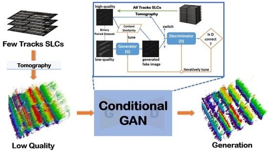
Flowchart of proposed method. The proposed method is composed of two main modules. The data generation module explains the generation of the super-resolution dataset that contains the paired low-quality and high-quality slice sets. The CGAN module illustrates the dominant compositions of the CGAN model and the data flowpath.
Remotesensing 13 05055 g002
Figure 3. Diagram of TomoSAR imaging geometry. TomoSAR expands the spatial resolution in the elevation direction by coherent antenna phase centers (APCs), represented as a series of black points.
Remotesensing 13 05055 g003
Figure 4. Flowchart of TomoSAR imaging procedure. The procedure contains a series of operations. Firstly, the image registration ensures the azimuth-range units in different coherent SAR images related to the same scatterers. Secondly, the channel imbalance calibration compensates the phase errors among channels. Thirdly, sparse recovery methods are applied to invert the elevation position of scatterers. Finally, the coordinate system is transformed from radar system to the geodetic system.
Remotesensing 13 05055 g004
Figure 5. Flowchart of data generation. The final output is the paired super-resolution dataset composed of low-quality and high-quality slice sets. The low-quality set of low-SNR and low-resolution contains range-elevation 2D binary slices, which is generated from three tracks. In contrast, the high-quality set uses all tracks, and has high SNR and resolution. The binary operation means that the value set is 1 if a scatterer is estimated in this position. All slices are in radar coordinate system.
Remotesensing 13 05055 g005
Figure 6. Flowchart of the CGAN module. The CGAN consists of two models named generator (G) and discriminator (D). The generator produces a fake result as similar as possible to the ground truth to make the discriminator believe the generation is the truth. On the contrary, the discriminator is used to distinguish the fake result and ground truth. After iterations, the generator will be able to generate a refined result which is hard to tell from the corresponding ground truth. Besides this, the content loss between the generated result and ground truth is also considered avoiding position bias.
Remotesensing 13 05055 g006
Figure 7. Network structure of the generator. The generator is composed of three dominant parts: downsampling compression, feature extraction, and upsampling reconstruction. The downsampling compression part compresses the data dimension and expands the feature dimension from 64 to 256. The feature dimension is indicated by the number on the left side of blocks, such as n128. The feature extraction part is composed of nine stacked blocks based on res-net structure, which has capability of digging out high-dimensional features of data. The upsampling part decreases the feature dimension and reconstructs the data dimension by deconvolution (TransposedConv) layers.
Remotesensing 13 05055 g007
Figure 8. Network structure of the discriminator. The network contains four convolutional layers increasing the feature dimension from 64 to 512, and finally becomes 1 to indicate the truth possibility of a small area in the receptive field. In the first four layers, the BatchNorm model is inserted into layers to accelerate the convergence and the LeakyReLU model is used as the activation function.
Remotesensing 13 05055 g008
Figure 9. Optical and intensity SAR images of YunCheng data. Panel (a) is the optical image of target scene including nine buildings in total. Each of the buildings is indicated using rectangles and numbered in the top-left corner. Panel (b) is the SAR image covering the same scene. The buildings in the SAR image are indicated with rectangles and are numbered correspondingly. Besides, two buildings marked with red rectangles at the bottom-right of the images are selected as training set. The other buildings with white rectangles are the testing set. Moreover, buildings #3, #4, and #5 are strongly overlapped in the SAR image and buildings #6, #7, #8, and #9 are nonoverlapped buildings. Slice 1 and slice 2 are selected at two azimuth positions to explain the results by different methods of overlapped and nonoverlapped buildings.
Remotesensing 13 05055 g009
Figure 10. 3D reconstruction results of all-track and three-track TomoSAR. Panel (a) is the 3D height distribution of all-track TomoSAR scatterers. The buildings can be easily distinguished. The structures of buildings are refined. Panel (b) is the normalized strength distribution of all-track TomoSAR. The dominant scatterers mainly locate at the surface of buildings. Panel (c) is the height distribution of three-track TomoSAR. The structures of buildings are fuzzy. Besides, there are also lots of artifacts and outliers. Panel (d) is the normalized strength distribution of three-track TomoSAR. Compared with all-track results, the strength distribution is worse with lots of powerful artifacts and outliers, which makes the height distribution of buildings fuzzy and declines the quality of reconstruction.
Remotesensing 13 05055 g010
Figure 11. Results of nonoverlapped buildings #6, #7, #8, and #9 reconstructed by all-track and three-track TomoSAR at slice 1 position. Panel (a) is height map of all-track TomoSAR. The identity numbers of buildings are placed near the corresponding ones. Panel (b) is the normalized strength map of all-track TomoSAR. Panel (c) is the height map of three-track TomoSAR and (d) is the normalized strength map of three-track TomoSAR. The heights of four buildings are estimated from the strength maps and indicated by orange lines at the top of buildings. Compared with all-track TomoSAR results, the results of three-track TomoSAR have more artifacts and outliers with stronger power. The structures become blurry and are affected by the powerful multipath scattering (marked with red circles).
Remotesensing 13 05055 g011
Figure 12. Results of nonoverlapped buildings #6, #7, #8, and #9 reconstructed by CGAN and nonlocal methods using three tracks at slice 1. Panel (a) is the height map of CGAN. Panel (b) is the normalized strength map of CGAN. Panel (c) is the height map of the nonlocal algorithm. Panel (d) is the normalized strength map of the nonlocal algorithm. The nonlocal algorithm can remove the artifacts and outliers by increasing the SNR. However, it is still affected by the multipath scattering, marked with red circles. In contrast, the proposed CGAN method generates a higher quality result by suppressing more artifacts and outliers. In addition, the multipath scattering is also well suppressed so that the structures are much clearer. The height estimations are also labeled with orange lines.
Remotesensing 13 05055 g012
Figure 13. Results of overlapped buildings #3 and #4 reconstructed using three and all tracks at slice 2 position. Panel (a) is the height map of all-track TomoSAR. The identity number of buildings is placed near the corresponding ones. Panel (b) is the normalized strength map of all-track TomoSAR. Panel (c) is the height map of three-track TomoSAR. Panel (d) is the normalized strength map of three-track TomoSAR. The buildings #3 and #4 are overlapped in the SAR image. From results of three-track TomoSAR, the overlapped two buildings cannot be distinguished from each other; the structure of building #3 is too blurry to tell it apart from building #4. Moreover, the top of building #3 is hard to determine, and it is impossible to estimate its height. The height estimation is labeled with orange lines.
Remotesensing 13 05055 g013
Figure 14. Results of overlapped buildings reconstructed by nonlocal algorithm and proposed CGAN methods. Panel (a) is the height map of the nonlocal algorithm. Panel (b) is the normalized strength map of the nonlocal algorithm. Panel (c) is the height map of the proposed CGAN method. Panel (d) is the normalized strength map of the proposed method. Generally, the nonlocal algorithm can divide two overlapped buildings with an obvious interval. However, there are still some artifacts and outliers. In contrast, the results of the proposed method can greatly distinguish between two buildings with a large interval. Additionally, the roofs of two buildings are clear. The height of building #3 estimated in the height map of the proposed method is closer to ground truth. The height estimation of building #3 in the nonlocal result is severely different from that of all-track results, which is probably affected by the multipath scattering. The height estimation is labeled with orange lines.
Remotesensing 13 05055 g014
Figure 15. Comparison of entire scene 3D reconstruction between the nonlocal algorithm and proposed CGAN method. Panel (a) is the reconstruction result of the nonlocal algorithm. Panel (b) is the reconstruction result of the proposed CGAN method. Comparatively, the quality of the CGAN method is higher with fewer artifacts and outliers. In addition, the structures of buildings are much clearer, and are closer to the results of all-track TomoSAR.
Remotesensing 13 05055 g015
Figure 16. Optical and SAR intensity images of spaceborne data. Panel (a) is the SAR intensity image of the building. The red line is the slice selected to show details. Panel (b) is the corresponding optical image.
Remotesensing 13 05055 g016
Figure 17. 3D views of reconstruction by CS method using all tracks and three tracks. Panel (a) is the 3D view of reconstruction using three tracks. There are lots of outliers. Panel (b) is the 3D view of reconstruction using all tracks. There are few outliers and the surface of the building is clean and refined.
Remotesensing 13 05055 g017
Figure 18. Reconstruction results of CS method using three and all tracks at the position indicated by the red line in the SAR intensity image. Panel (a) is the height map of three-track TomoSAR. Panel (b) is the normalized strength map of all-track TomoSAR. The orange circles indicate the outliers. Panel (c) is the height map of all-track TomoSAR. Panel (d) is the normalized strength map of all-track TomoSAR. The orange lines mark the height of the building. There are lots of outliers in the three-track reconstruction result.
Remotesensing 13 05055 g018
Figure 19. Reconstruction results of the nonlocal algorithm and the proposed CGAN methods. Panel (a) is the height map of the nonlocal algorithm. Panel (b) is the normalized strength map of the nonlocal algorithm. Panel (c) is the height map of the proposed CGAN method. Panel (d) is the normalized strength map of the proposed CGAN method. Generally, the nonlocal algorithm can compress the outliers. In contrast, the proposed CGAN method can further compress the outliers and generate more refined surface. The orange lines mark the height of the building.
Remotesensing 13 05055 g019aRemotesensing 13 05055 g019b
Figure 20. 3D views of reconstruction results of the nonlocal algorithm and the proposed CGAN method. Panel (a) is the 3D result of the nonlocal algorithm using three tracks. There are also lots of outliers and the reconstructed surface is not smooth. Panel (b) is the 3D result of the proposed CGAN method using three tracks. There are few outliers and the surface of buildings is clean and refined. The CGAN, which is just trained on the airborne dataset, can effectively and robustly process the spaceborne dataset without any tuning.
Remotesensing 13 05055 g020
Table 1. Parameters of YunCheng airborne dataset.
All-TrackThree-Track
Number of tracks83
Maximal elevation aperture0.588 m0.168 m
Distance from the scene center1308 m
Wavelength2.1 cm
Incidence angle at scene center58°
Table 2. Configurations of nonlocal algorithm.
ParameterValue
search window size 9 × 9
patch size 3 × 3
iterations10
posterior similarity coefficient (h)5.3
sparse prior KL similarity 0.2× 9 × 9
minimum number of similar blocks ( L m i n )10
Table 3. Height estimation results by different methods.
Building_IndexAll Tracks3 Tracks\ErrorNonlocal\ErrorProposed\Error
#37589\1490\1575\0
#440Hard to recognize42\242\2
#68182\182\181\0
#77487\1387\1373\1
#89090\091\190\0
#99393\093\093\0
Table 4. Time consumption of different methods.
MethodTime Consumption (s)
Nonlocal (10 iterations)14,492
Proposed GAN10
Table 5. Parameters of TerraSAR-X spaceborne dataset.
All-TrackThree-Track
Number of tracks193
Maximal elevation aperture215 m42 m
Distance from the scene center617 km
Wavelength3.1 cm
Incidence angle at scene center66°
Publisher’s Note: MDPI stays neutral with regard to jurisdictional claims in published maps and institutional affiliations.

