Article

Multi-Hypothesis Topological Isomorphism Matching Method for Synthetic Aperture Radar Images with Large Geometric Distortion

School of Electronics and Communication Engineering, Shenzhen Campus of Sun Yat-Sen University, No. 66, Gongchang Road, Guangming District, Shenzhen 518107, China
*
Author to whom correspondence should be addressed.
Remote Sens. 2021, 13(22), 4637; https://doi.org/10.3390/rs13224637
Submission received: 27 September 2021 / Revised: 1 November 2021 / Accepted: 15 November 2021 / Published: 17 November 2021
(This article belongs to the Special Issue Remote Sensing and GIS for Geomorphological Mapping)

Abstract

:
The dramatic undulations of a mountainous terrain will introduce large geometric distortions in each Synthetic Aperture Radar (SAR) image with different look angles, resulting in a poor registration performance. To this end, this paper proposes a multi-hypothesis topological isomorphism matching method for SAR images with large geometric distortions. The method includes the Ridge-Line Keypoint Detection (RLKD) and Multi-Hypothesis Topological Isomorphism Matching (MHTIM). Firstly, based on the analysis of the ridge structure, a ridge keypoint detection module and a keypoint similarity description method are designed, which aim to quickly produce a small number of stable matching keypoint pairs under large look angle differences and large terrain undulations. The keypoint pairs are further fed into the MHTIM module. Subsequently, the MHTIM method is proposed, which uses the stability and isomorphism of the topological structure of the keypoint set under different perspectives to generate a variety of matching hypotheses, and iteratively achieves the keypoint matching. This method uses both local and global geometric relationships between two keypoints, hence it achieving better performance compared with traditional methods. We tested our approach on both simulated and real mountain SAR images with different look angles and different elevation ranges. The experimental results demonstrate the effectiveness and stable matching performance of our approach.

Graphical Abstract

1. Introduction

About 24% of the earth’s land is covered by mountains [1]. Since NASA launched its first SAR satellite SEASAT in 1978, several countries have successively deployed multiple spaceborne SAR systems, accumulating massive amounts of SAR image data of mountain areas. In order to jointly exploit these data for elevation inversion, deformation detection, and biomass monitoring, an accurate matching performance becomes a prerequisite. However, the SAR imaging mechanism determines that a mountainous SAR image is a slope-distance mapping of the mountain from a three-dimensional space to a two-dimensional image. The difference in the viewing angles causes a relative geometric distortion between two images. In particular, the larger the difference in the angles, the larger the geometrical deformations. This poses great challenges to the registration of SAR images with large geometric distortion.
Increasing efforts have been made to improve the accuracy of registration. According to a measuring function, an acceptable classification [2] for existing SAR image matching methods is area-based [3,4,5,6,7,8,9] and feature-based [10,11,12,13,14,15,16,17] pipelines. The area-based methods either use image grayscale statistical information or transform domain statistical information as a measure, and register the image by searching for the maximum value of the measuring function. These types of methods are more suitable for the cases with a small difference in look angles, that is, the cases where the coherence between images is high, and widely used in interferometric SAR (InSAR) [18,19] and SAR tomography (TomoSAR) [20,21]. However, this type of SAR image accounts for only a small proportion. Since the topography of the imaging area increases sharply with increasing difference in SAR imaging angles, the relative deformations of the images increase and the correlation between them decreases. In this case, a feature-based method is more suitable. The feature-based methods first extract spatial features such as corners, contours, and line segments in an image, then produce homologous points by some matching methods, and finally calculate a transfer model between images based on the homologous points, so as to complete the matching. Among many feature-based methods, the Scale-Invariant Feature Transform (SIFT) [10] is the most widely used method. It is capable of coping with geometric transformations, such as scaling and rotation. However, its real-time performance is limited, and it cannot handle smooth edges well. Based on SIFT, Speeded-Up Robust Features (SURF) [16] use the Haar wavelet response and integral image to improve the computational efficiency. However, the performances of SIFT and SURF in SAR image matching are still not very satisfactory. In order to reduce the impact of coherent speckle on the SAR image processing, Dellinger et al. [12] proposed the SAR-SIFT method based on a new gradient definition. Subsequently, Ma et al. [22] proposed an improved SIFT and enhanced the feature matching method named PSO-SIFT to enhance the adaptability of features. Xiang et al. [23] proposed a high-level rotation invariant descriptor that does not specify the master direction to improve SIFT, and improved the discrimination of different feature descriptors. Apart from the SIFT-like methods, DASIY, BRIEF, ORB and other methods [24] also complete the optical image registration under small differences in viewing angles.
Most of the existing approaches work on the improvement of general feature descriptors. The matching algorithms for large geometric deformation of SAR images are still in their infancy. Although SAR-SIFT and PSO-SIFT [12,22] have achieved good results for mountain SAR image registration with small differences in viewing angles, they remain challenging when registering large geometric distortion of SAR images with only a small number of keypoints (refer to the experimental part in Section 3 for detail). For small-deformation SAR image registration, fewer keypoints can complete a global high-precision fitting of the matching transformation model. However, it is difficult for a matching transformation model of large distortion of SAR images to perform a global high-precision approximation through a linear affine transformation and a low-order nonlinear transformation. In this case, it is important to know how to improve the quality and quantity of keypoints, so as to increase the matching accuracy.
The ridge is one of the cardinal topographic features, which forms the skeleton line of an undulating topography and reflects the spatial topological structure of the topography. For solving the problem of large geometric distortion of SAR image matching in mountainous areas caused by large differences in look angles and severe terrain fluctuations, we propose a large geometric distortion SAR image multi-hypothesis topological isomorphism matching method. It is composed of keypoints of ridges Detection (Ridge-Line Keypoint Detection, RLKB) and Multi-hypothesis Topological Isomorphism Matching (MHTIM). The method can produce more matching keypoints with better stability, so as to achieve a higher matching precision.
This paper is arranged as follows. In Section 2, we introduce the motivation and ideas of the proposed method and discuss the two parts of the method in detail. In Section 3, we present the simulation results and measured data. Finally, in Section 5, we summarize the method and give directions for future improvements.

2. Methods

The overall flowchart of our proposed method is shown in Figure 1. In the rest of this section, we first analyze the deficiency of existing methods and present the motivation of the proposed method in Section 2.1, and then explain RLKB and MHTIM in Section 2.2 and Section 2.3, respectively.

2.1. Problem Description

Despite its long success in optical image matching, the feature-based method still has vulnerability in detecting and matching the ridge features of most of the parts of SAR images with large geometric distortion. In the case of a SIFT-like method, there are two reasons: (1) The method constructs the Difference of Gaussian (DoG) pyramid of the image when considering the image scale. The position of the keypoints in the image has an offset relative to that of the ridge. So, the keypoints cannot represent the position of the ridge. (2) The method generally uses information such as the gray gradient direction of the small image blocks around the keypoint as the descriptor, and calculates the similarity of the descriptor (distance between two vectors) to determine whether the keypoints represent a homologous object. In fact, in mountain areas, when the look angle of the SAR image changes significantly, except for the ridge line with a larger scale, other areas of the image have significant changes in brightness, shape and even phase, which make the similarity of the descriptor invalid. Similar to the intuitive experience, the topological structure of the ridge features in the SAR image at different look angles is isomorphic.
Analyzing Figure 2, it is observed that the distributions of the extreme points of the image intensity formed by SAR images with different look angles on ridges are isomorphic. Figure 3 shows the SAR image of the mountainous area of the Sichuan-Tibet Plateau in China, where the DEM data of the DEM map, ascending stripe mode SAR image from Sentinel 1 and descending stripe mode SAR image from Sentinel 1 are shown in a–c, respectively. Sub-figures a–c in Figure 3 have undergone rough geometric registration. It is worth mentioning that geometric registration can roughly overlap the regions to be registered to enhance the efficiency of subsequent algorithms, and when the images overlap (like the images produced by TanDEM-X), geometric registration is not necessary. In Figure 3, two images are taken from the opposite-side of the terrain, and the angle between the line of sight of (b,c) is greater than 90°. We can find even more intuitively that when SAR images are taken from opposite-side, the topological structures composed of yellow circles and yellow lines in the three figures are still isomorphic. Therefore, this paper attempts to match the ridge features through the topological relationship between the ridge features. It divides the method into two parts: ridge keypoint detection and matching.
In geometry, the feature information that characterizes the mountain morphology includes extreme points, saddle points, ridge lines, valley lines, etc. [25]. The most apparent feature in mountain SAR images is the ridge line and the intersection of two or more ridge lines. Since the SAR image is a slant distance mapping from a three-dimensional space to a two-dimensional image, it is necessary to find a stable ridge line detection method. The ridge line is a kind of edge information. Commonly used edge detection operators include algorithms such as Sobel, LoG, Canny, etc. [26], followed by deep learning methods such as Holistically-nested Edge Detection (HED) [27] and Richer Convolutional Features (RCF) [28]. The location of the intersection of lines is generally obtained by calculating its surrounding curvature, gradient, etc. [13]. However, the time complexity of the above methods is relatively high. This paper proposes a ridge feature keypoint detector based on the LoG operator, which can produce stable ridge keypoints while detecting ridge lines at a lower time complexity.
The keypoint matching is a key step to complete image matching. Existing feature-based pipelines generally use some algorithms to solve the assignment problem [29] after calculating the similarity matrix of the master and slave image descriptor sets, and then use the RANdom SAmpling Consensus (RANSAC) [30] algorithm for outlier culling. This type of pipelines generally pays attention only to the similarity between keypoint descriptors (the distance between vectors) and ignores the inherent geometric topological relationship between the keypoints. Although RANSAC is simple and clear algorithm, the calculation cost in its iterative process is relatively large and the optimal solution cannot always be found [31].
Analyzing Figure 3, it is found that the distributions of the extreme points of the image intensity formed by SAR images with different look angles on ridges are still isomorphic. Therefore, this paper proposes a Multi-Hypothesis Topological Isomorphism Matching (MHTIM) method. This method converts the stable keypoint matching pairs generated by RLKD into an initial topological structure graph hypothesis according to its topology. Based on this, the method iteratively introduces the remaining unmatched keypoints to form a hypothesis tree. When the hypothesis tree reaches a certain depth, the hypothesis score is calculated, and the hypothesis tree is pruned to gradually complete the matching process.

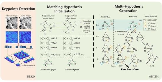
2.2. Ridge Line Keypoint Detection Method

The RLKD method is divided into three parts: (1) Quick detection of the ridge line intersection point, which ridge detection is performed in the distance and azimuth direction, respectively, to quickly obtain the ridge intersection point; (2) keypoint generation and description, which cluster the intersection point pixels to produce the keypoint, and a keypoint descriptors are designed to measure their similarity; and (3) fast matching, which calculates the distance matrix of ridge keypoints through the descriptor, and uses the simulated annealing algorithm to solve the two-allocation problem for obtaining a small number of stable keypoint matching pairs. As there exist many mathematical operators in the following passage, for convenience, we define all the notations in Table 1.

2.2.1. Quick Detection of Intersection of Ridge Lines

Our method is based on the LoG to rapidly detect the intersection of ridge lines by using two detectors r D e c (Detector in range) and a D e c (Detector in azimuth), which are defined as follows:
r D e c = 2 r 2 G r , a , σ = r 2 σ 2 σ 4 e r 2 + a 2 2 σ 2 a D e c = 2 a 2 G r , a , σ = a 2 σ 2 σ 4 e r 2 + a 2 2 σ 2
Among them, G r , a , σ is a two-dimensional Gaussian filter:
G r , a , σ = 1 2 π σ 2 e r 2 + a 2 / 2 σ 2
In the above formula, σ is the standard deviation. Due to the low-pass characteristics of the Gaussian filter, fine textures can be eliminated and large-scale ridge features can be retained while suppressing the influence of coherent speckles. In addition, if not otherwise stated, r and a represent the distance pixel index and azimuth pixel index of the image, respectively. Next, the intersection point is obtained based on the detected ridge line. Assuming that the image gray function is I, I r D e c and I a D e c as the responses of I can be obtained through a D e c and r D e c as follows:
I r D e c = I r D e c , I a D e c = I a D e c
where ∗ is the convolution operation. The edges of the image along the distance and the azimuth directions exist at the position where the two adjacent pixel values have different signs. The results of edge detection along the two directions can be produced by using the following two equations:
I r e ( r , a ) = 0 , I r D e c ( r , a ) · I r D e c ( r , a + 1 ) 0 1 , I r D e c ( r , a ) · I r D e c ( r , a + 1 ) < 0 I r a ( r , a ) = 0 , I a D e c ( r , a ) · I a D e c ( r + 1 , a ) 0 1 , I a D e c ( r , a ) · I a D e c ( r + 1 , a ) < 0
The pixel with value of 1 in I r e and I r a is the edge. Now, I r e and I r a are to be superimposed, that is:
I E = I r e + I r a
I E represents the final edge detection result. In I E , the pixel with the value greater than 0 is the ridge, and the pixel with the value of 2 is the intersection of the ridge lines.

2.2.2. Keypoint Generation and Descriptor

A real ridge intersection generates a concentrated area in I E with a value greater than 1, which contains a lot of information about the ridge intersection. This paper uses the block of this area as a keypoint descriptor, clusters these pixels, and uses the cluster center as the keypoint. Suppose that in I E , the number of intersections generated is T, and k i = r i , a i are the coordinates of the intersection in the image, where i = 1 , 2 , , T . For the first intersection, a traversal search is performed on the image block centered on this point with a fixed radius, any other intersection in the image block will center on itself, continue to search for other intersections within the same radius, and cluster to C. Additionally, C j represents the set of subscripts of the intersection points contained in the jth cluster. Equation (6) can be used to calculate the jth cluster center, which is the keypoint required by the algorithm in this paper:
v j = 1 C j i C j k i
This paper uses a R × R 9×9 I E block s with the keypoint position as the center of the keypoint descriptor, where R is the block size, which we set to 9. This descriptor retains the shape information of the ridge line around the keypoint. For two image blocks, the measures of similarity include correlation, mutual information and cross entropy. The correlation and mutual information are two basic and effective methods of similarity measurement. The cross entropy [32] has high robustness and it is widely used in the loss function in the framework of deep learning algorithms. However, it is usually used to calculate the similarity of multi-spectral images with complex textures. As shown in Table 2, for SAR images with large geometric distortion, we get the best result by using cross-correlation as the descriptor similarity measurement method. The reason is explained in more detail in Table 2 in Section 3. In particular, the larger the maximum value of the correlation coefficient, the more similar the descriptors. Therefore, our method uses the maximum value of the correlation coefficient to represent the similarity between two descriptors, which is defined as follows:
d s 1 , s 2 = max C s 1 , s 2
In the above formula, C is the real correlation coefficient matrix of descriptors s 1 and s 1 , obtained by using formula (8), where represents the conjugate operation and R is the block size of s:
C s 1 , s 2 = u = 1 R v = 1 R r = 1 R a = 1 R s 1 r , a e 2 j π u r + v a R · r = 1 R a = 1 R s 2 r , a e 2 j π u r + v a R e 2 j π u r + v a R
In Figure 4, we show the SAR-SIFT keypoint detection results of the SAR image pair in the mountain area under the typical parameters reported by Dellinger et al. [12]. We present the keypoint detection and description results of our method in Figure 5. We can find in Figure 4 that the detection results of keypoints in the mountain area, obtained by the SAR-SIFT method, have two characteristics. Firstly, for images with different look angles, the number of characteristic points is obviously different, and second, the keypoints mainly exist on the back slope and are not even.
Figure 5a,b show the ridge line and keypoint detection results of the SAR image shown in Figure 4a,b, respectively. In (a,b), the green line is the detection result of the ridge line, and the yellow dot is the keypoint before clustering; (c,d) are corresponding results after clustering. The red boxes marked in (a,b) and (c,d) are the positions of the manually selected keypoints to reveal the descriptor and enlarged patches in the 3rd row. Keypoints 1 and 2 of the master image correspond, respectively, to Keypoints 1 and 2 of the same ground object in the slave image. The 4th row shows the calculated maximum value of the two-dimensional correlation coefficient of the descriptor. It can be seen that the maximum values of the correlation coefficient between keypoint 1 of the master image and keypoints 1 and 2 of the slave image are 0.86 and 0.74, respectively; while the maximum correlation coefficients between keypoint 2 in the master image and keypoints 1 and 2 in the slave image are 0.64 and 0.84, respectively. That is, keypoint 1 of the master image matched more with keypoint 1 of the slave image, and keypoint 2 of the master image matched more with keypoint 2 of the slave image, which is in line with the actual situation. Figure 5 shows that the descriptor designed in this paper describes the similarity of keypoints effectively.

2.2.3. Quick Matching

Assuming that M and N keypoints are detected in the master and slave images, respectively, an M × N -dimensional similarity matrix can be generated as D = d s i , s j | i = 1 , 2 , . . . , M , j = 1 , 2 , , N , where s is the keypoint descriptor. Finding the best match between the keypoints of the master and slave images in the similarity matrix is a typical optimization problem. Our method uses the simulated annealing algorithm [33] to solve the optimization problem. Finally, the method proposed in this section still uses the RANSAC [30] algorithm to delete outliers of matched pairs, and quickly finds stable keypoints. It is worth mentioning that the application of the transformation model to the image distortion mode in the RANSAC algorithm is very important for the registration result. The two most basic transformation models, used in the task of large-distortion SAR image registration, are projection transformation and affine transformation. For more complex scenes, polynomials can be used to fit a transformation model. Since the geometric distortion of a SAR image is more in the slant range direction, the Local Weighted Mean (LWM) [34] transformation model is used. The LWM model introduced by Goshtasby [34] is capable of the condition when parts of the image appear distorted differently, and the distortion varies locally and piecewise in a nonlinear manner.
In Section 3, we compare the pros and cons of several models, and verify that the LWM model is indeed the most suitable model for the scenario targeted in this article.

2.3. Multi-Hypothesis Topological Isomorphism Matching Method

The main aim of the MHTIM method is to transform the stable keypoints matching from RLKD into two initial graph hypotheses according to their topological structures. Based on the ridge feature topological isomorphism, it iteratively adds the remaining unmatched keypoints to form a hypothesis tree. When the hypothesis tree reaches a certain depth, the hypothesis score is calculated. Then, the hypothesis tree is pruned according to the score, and subsequently the matching process is completed.
In this section, we first introduce the initialization of the hypothesis tree and the sorting of candidate points. The subsequent iteration process is introduced one by one in three steps as follows:
  • Multi-hypothesis generation: According to the ranking results, select the top candidate keypoints and add them to the graph to generate new hypotheses.
  • Hypothesis score calculation: We use five graph indicators and node angle similarity indicators to rank the new hypotheses. The hypothesis that ranks first in a single indicator gets a certain score. The final score of a new hypothesis is the sum of the scores assumed under each indicator.
  • Pruning: New hypotheses are sorted in terms of their final scores, pruning low-scoring hypothesis branches, retaining high-scoring hypothesis branches, and updating the root node, matching, and candidate point sets.
A schematic diagram of the above steps is shown in Figure 6. Through the above steps, the keypoints that are not matched but have potential matches are gradually added to the matching set.

2.3.1. Hypothesis Initialization and Candidate Keypoints Sorting

Before starting iterations, the MHTIM method first initializes the root node of the hypothetical tree. The specific process is shown in Figure 7.
We use v = r , a to represent the coordinates of the keypoint in the image. Suppose that after RLKD, keypoints detected in the master and slave images are defined as point sets V m = { v i m } ; i = 1 , , N m and V s = { v j s } ; j = 1 , , N s , respectively. After the RLKD algorithm quick matching, V m and V s are divided into two parts: matching point set V matched m = { v k m } and V matched s = { v k s } ; k = 1 , , r , and candidate point set V unmatched m = { v p m } ; p = r + 1 , , N m and V unmatched s = { v q s } ; q = r + 1 , , N s . D m = d i 1 , i 2 r × r and D s = d j 1 , j 2 r × r are the putative self-distance matrices of V matched m and V matched s , respectively, where d i 1 , i 2 = v i 1 m v i 2 m 2 and d j 1 , j 2 = v j 1 s v j 2 s 2 .
First of all, this article quickly matches the keypoint pair initialization, generates the master and slave undirected weighted graphs G m and G s , respectively, and v m and v s are regarded as nodes in G m and G s , respectively. After that, if d i 1 , i 2 or d j 1 , j 2 is greater than ε , an edge e i 1 , i 2 m = ( v i 1 m , v i 2 m ) or e j 1 , j 2 s = ( v j 1 s , v j 2 s ) is generated, where ε is the threshold value set according to the number of pixels in the image. Generally, ε is set to one half of the diagonal length of the image as follows:
ε = 0.5 h 2 + w 2
In the above formula, h and w are the number of pixels of the image in the range and azimuth directions, respectively. As shown in Figure 7, the master and slave initial graphs show strong topological isomorphism. Please note that the distance in Figure 7 is the unitless distance after a normalization operation, and ε is scaled in the same proportion.
We sort the candidate points by S to ensure the quality of the hypothesis generated by the selected candidate points in each iteration of the algorithm. The definition of S is as follows:
S ( p , q ) = 1 ζ m × v p m v V matched m v V matched m 2 v q s v V matched s v V matched s 2 × 1 ζ s
The right-hand side of Equation (10) contains the first and second normalized value terms, in which the distance from the candidate point v p m of the master image to the geometric center of the matching keypoint set V matched m , and the distance from the candidate point v q s of the slave image to the geometric center of the matching keypoint set V matched s . ζ m and ζ s are the normalization factors, which are set according to the area covered by the image on the ground and size of the image:
ζ = h 2 + w 2 L r 2 + L a 2
where, L r and L a are the length with a unit of meter of the area covered by the image on the ground in the range and azimuth direction, respectively. It is worth mentioning that when the master and slave images are geometrically registered and their scales are the same, ζ m and ζ s can be set to 1 at the same time.
Equation (10) can be understood in terms of the similarity of the distance from the candidate keypoints in the master and slave images to the respective geometric centers. The higher the similarity, the more likely the two candidate keypoints represent the same ridge feature.

2.3.2. Multi-Hypothesis Generation

Referring to Figure 6, we assume that the maximum depth of the tree is H = 3 , and the leaf nodes of the tree generate at most W = 2 new hypothetical nodes at each iteration to illustrate the iteration process. After initialization, suppose that at the beginning of the ( k 3 ) th iteration, the root graph of each of master and slave trees has 4 nodes (as shown in the ( k 3 ) th layer in Figure 6). After the first ( k 2 ) iterations, the first node v 1 s t m in the sequence of the remaining candidate keypoints after sorting in the master graph is added to G m . For the slave tree, the two points in V u n m a t c h e d s with the highest similarity to v 1 s t m are added to G s to form two hypotheses. At this point, the depth of the target hypothesis tree from the root node is 2. The above steps are reproduced sequentially in the ( k 1 ) th and kth iterations. At k, the target hypothesis tree has a depth of 4, and there are at most 8 leaf nodes in the fourth layer. So far, in this example, the hypothesis tree has been generated.
We can find that the hypothesis tree retains multiple matching combinations. The following steps are to calculate the scores of the hypotheses for evaluating their qualities, and for pruning the hypothesis tree so as to remove the low-quality hypotheses and retain the correct ones.

2.3.3. Hypothesis Score Calculation

The score of a hypothesis comes from the similarity of the newly added vertices of the master and slave hypotheses. We use 5 common graph indicators and a custom indicator of the newly added nodes in the graph to measure the similarity of hypotheses. The five graph indicators are node centrality, betweenness centrality, proximity centrality, K kernel number, and eigenvector centrality. In addition to the above general graph indicators, the use of geometric constraints can enhance the matching accuracy of graph nodes in a realistic scene [35]. We define a node angle similarity index. First, an angle vector is used to describe the position of a node in the graph relative to the rest of the nodes. The vector is defined as:
Φ v i , G = ϕ l , ϕ l = arctan v i v l , v l G , v l v i
After that, the node angle similarity α ( p , q ) is defined in terms of the mean absolute value of the difference between the angle vectors of the newly added vertices of the master and slave graph, namely:
α ( p , q ) = | | Φ ( v p m , G m ) Φ ( v q s , G s ) | | 2 | G m | 1
where | G m | represents the number of nodes in the master graph at the kth iteration.
After the calculation of the 6 indicators of the newly added nodes is completed, we rank each hypothesis according to the similarity of each indicator.
After we get the 6 index values of the newly added vertices of the new hypothesis, we sort each new hypothesis according to the similarity of each index. The hypothesis that ranks high in an indicator gets a certain score, and the final score of the hypothesis is the sum of the scores on each indicator.

2.3.4. Pruning

The purpose of pruning is to remove hypotheses with lower scores in the hypothesis tree, and to update the root node to output a new pair of matched keypoints. After obtaining the hypothesis score at the kth iteration, the branch that does not contain the highest scoring hypothesis is deleted. After that, the k-H layer node of the reserved branch is used as the new root node, and the matching point which added by this node is output to V matched m and V matched s . Finally, the point is deleted from V unmatched s and V unmatched s , and the next iteration is started.
After all unmatched keypoints participate in the iterative process, the MHTIM terminates the iteration process and outputs the final hypothesis with the highest score. At this point, all the vertices in the master and slave graphs correspond one-to-one, and the final matching pair set C = v k m , v k s , k = 1 , 2 , . . . , r is formed.

3. Experiment

In this section, we use both simulated and measured data to verify the performance of the two steps of our proposed method. The simulated data simulates a pair of SAR images in mountain areas and different look angles to verify the matching effect of our method under different look angles. The measured data is used to verify the matching effect of our method for different types of terrain SAR images under the same difference in look angles. We compare the performance of our method with those of SAR-SFIT and PSO-SIFT to show that our method is more suitable for SAR images with large geometric distortion matching than these two methods. More specifically, we compare the Mean-Absolute Error (MAE) of matching results of these algorithms, Number of Keypoints Matched (NKM), and Proportion of Keypoints Matched (PKM) to demonstrate the pros and cons of these algorithms.

3.1. Data Set

The simulated SAR data is generated by the Space-borne Radar Advanced Simulator (SRAS) system [36,37]. This batch of data is shown in Figure 8. It is a simulation of four types of mountain terrains. The size is 512 × 512 pixels, and the range and azimuth resolution is about 1 m. From area 1 to area 4, their elevation ranges are 350 m–470 m, 320 m–470 m, 390 m–550 m, and 395 m–570 m, respectively. Their look angles are 15 ° , 20 ° , 25 ° , 30 ° , and 40 ° , respectively. The measured data are taken from the TerraSAR-X system, which are L1A-level SAR images collected in the Alps and its vicinity. Master images were collected on 12 January 2009, with a look angle of 35.8153 ° , and slave images were collected on 9 December 2008, with a look angle of 20.7765 ° . As shown in Figure 9, we use four terrain image blocks with a size of 512 × 512 pixels.

3.2. Implementation Details

Refer to Dellinger et al. [12] and Ma et al. [22] for SAR-SIFT and PSO-SIFT, respectively. When constructing the scale space, use the initial scale δ = 2 , ratio coefficient k = 1.26 , and number of scale space layers N m a x = 8 . The arbitrary parameter d of the SAR-Harris function is set to 0.04, and the threshold is set to 0.8. For RLKD, we set the radius of the search space to 5. For the SAR image after geometric registration, the feature scale and direction in the image are almost the same. Therefore, the standard deviation of the Gaussian function of the algorithm in this paper is set to σ = k N m a x 1 for producing large-scale features. In addition, for SAR-SIFT, PSO-SIFT and the method proposed in this paper, the LWM model is set as the default transformation model between the reference and the image.
We tested all the programs on an Ubuntu 18.04 system computer with 128 GB RAM, which is equipped with an Intel i9-9700X CPU and two Nvidia RTX3090 graphics cards.

3.3. Evaluation Index

  • Mean-Absolute Error (MAE):
    MAE is capable to measure the alignment error of keypoints, which is defined as follows:
    MAE = v i m , v j s C v i m Γ v j s 2 C
    where, Γ is the transfer model, and C is the number of keypoint pairs that are correctly matched, that is, NKM.
  • Number of Keypoints Matched (NKM):
    We use the final number of matching keypoints generated by each method as the number of keypoints matched to measure the effectiveness of the transfer model fitting.
  • Proportion of Keypoints Matched (PKM):
    In order to evaluate whether the keypoints detected by the method are efficient, we also use PKM as one of the evaluation indicators. PKM is defined as follows:
    γ = V matched s V s
    In the equation, V matched s represents the number of matching keypoints in the master image, and V s represents the number of all keypoints detected in the master image.

3.4. Result Analysis

In order to verify the performance of the algorithm in this paper, we designed the following experiments. First, in order to confirm the correctness of our choice of measurement function and transformation model in the algorithm, we designed the experiments and presented the results in Table 2 and Table 3. Second, in order to verify the pros and cons of the algorithm compared with other methods, we compared the MAE, NKM and PKM values of the registration results of the four methods on SAR images with different incident angle differences and different terrain undulations in Figure 8, Figure 9, Figure 10, Figure 11, Figure 12 and Figure 13. Then fusion result of our method on real data was showed in Figure 14. The rest of this section will provide a detailed discussion of the results of these experiments.
For the descriptors proposed in this paper, Table 2 shows the effect of using different similarity measurement functions on the fast matching results of RLKD on the simulation data set under a difference of 5 ° look angles. In Table 2, MCC is the abbreviation for the maximum value of the correlation function. We can observe that using the correlation function, the proposed method produces the smallest MAE and the largest NKM, but the average time is not increased significantly. Therefore, we choose the correlation function as the measuring function of the descriptor similarity in the RLKD step.
Table 3 shows the influence of different transformation models on the final matching results of our method for the simulated data set with a difference of 5 ° in look angles. It can be seen that after RLKD, the LWM model has the smallest MAE and the largest NKM, which are significantly better than those of other models. The similarity model is the simplest fitting model, but its result is the worst. The polynomial and affine models are worse than LWM, and the simplest similarity model is the worst. After MHTIM, increased NKM was produced by all the models. When the LWM model was used alone, the MAE of the matching results decreased. This is because, in the RLKD stage, the LWM model creates more stable matching result. The results presented in Table 3 also confirm our analysis in Section 3, that is, when registering mountain SAR images, the LWM model may achieve better results than other models.
Figure 8 shows the simulated data. In order to give an intuitive experience of the matching effects of different algorithms, and to take into account the clarity of the figure, this article shows only the matching keypoint results of the RLKD method and the SAR-SIFT in the figure. We can observe that compared to SAR-SIFT, the RLKD method achieves more matching points under large difference in look angles. It shows that the descriptors proposed in this paper are more suitable for the matching problem of mountain SAR images having large geometric distortion, which confirms the Section 2.1 of this paper. It also confirms that the ridge structure remains relatively unchanged in SAR images with different look angles.
Figure 10 shows the MAE values of the three registration algorithms for the simulated data under different differences in look angles. Among them, the MAE of SAR-SIFT is the largest, and the results are unstable in areas with different elevation differences. Overall, except for the case where DIA is equal to 25 ° in district 2, our method obtains the smallest MAE, and when the DIA increases, the MAE of the RKLD and MHTIM methods remain stable. This result shows that the method proposed in this paper can effectively overcome the geometric distortion caused by the large look angle difference and ensure the stability of the registration process. From the comprehensive analysis of NKM in Figure 11, it can be seen that for PSO-SIFT, the result of MAE is smaller than SAR-SIFT and its NKM is higher. But from the perspective of PKM in Figure 12, only about 10 % of the keypoints detected by PSO-SIFT are matched. This value is not higher than SAR-SIFT. This suggests that the keypoints detected by PSO-SIFT may not be more applicable than SAR-SIFT in SAR images with large geometric distortion. The MAE of RLKD in this paper is smaller than those of SAR-SIFT and PSO-SIFT. The RLKD+MHTIM method further reduces the MAE. This shows that the use of the isomorphism of the distribution structure of keypoints increases the stability of our method.
Figure 11 shows the NKM of the matching results of each method for the simulated data. Intuitively, PSO-SIFT is close to RLKD+MHTIM in district 1 and district 4, that is because these two areas have richer textures. The NKM of the RLKD method is between those of SAR-SIFT and PSO-SIFT, but the RLKD+MHTIM method greatly increases the NKM. Comprehensive analysis of Figure 10 and Figure 11 reveals that the RLKD+MHTIM method has the largest number of matching keypoint and the smallest error.
Figure 12 shows the PKM value of the matching results of each method for the simulated data. Except for district 3, the RLKD method produced slightly higher PKM values than SAR-SIFT and PSO-SIFT. However, the PKM value of the RLKD+MHTIM method is significantly higher than those of the other two methods.
In addition, the MAE of the matching result of the correlation-based method is shown in Figure 13. Since this method does not look for keypoints, we present only the MAE results. Compared with the feature-based method, the MAE of this method is at a higher level.
Figure 9 shows the measured TerraSAR-X image data. As in Figure 8, in order to give an intuitive experience of the matching effects of different algorithms and take into account the clarity of the figure, this paper shows only the matching keypoint results of the RLKD and SAR-SIFT methods. Figure 15 shows the histogram of NKM after matching the TerraSAR image data set with three methods. We can see that in the Mountain (Big) area with large terrain undulations, the number of matching keypoints produced by SAR-SIFT is less than that produced by our RLKD method and the distribution of keypoints is uneven. The performance of PSO-SIFT on this type of terrain is the most unstable. In the Mountains (Big) 1, 2 and 4 areas, the number of matching point pairs it obtains is less than one half of those obtained by the SAR-SIFT and RLKD methods. However, on the Mountains (Big) 3 area, the number of matching keypoint reached 39, surpassing SAR-SIFT’s 7 and RLKD + MHTIM’s 33. In the Mountains (Small) area with slightly smaller terrain undulations, NKM obtained by the RLKD method is slightly more than that of SAR-SIFT, and, more than that of PSO-SIFT except in area 3. The MHTIM method further matches the keypoints of the ridge detected by the RLKD method and produces at least twice the number of matching keypoints produced by the RLKD method.
In the areas of towns and others where the terrain is less undulating and more common, the NKM obtained by the RLKD+MHTIM method still has an absolute advantage over those of PSO-SIFT and SAR-SIFT, which proves that the RLKD+MHTIM method proposed in this paper is not only effective and efficient in matching SAR images with large geometric distortion, but also has advantages in registering general types of SAR images.
Finally, Figure 14 shows the matching and fusion results of the TerraSAR-X data based on the RLKD + MHTIM method. The shape of a grid can be seen in every plot because we use “checkerboard” display mode. We can find that in the mountain area, the shape of the ridge in the center of the image fits well. In areas with small terrain undulations, roads, rivers and other terrains on the ground are well matched, which proves that our method has good effectiveness to different types of terrains.

4. Discussion

In this paper, a Ridge Line Keypoint Detection (RLKD) method and a Multi-Hypothesis Topological Isomorphism Matching method (MHTIM) are proposed to match SAR images with large geometric distortion. We designed adequate experiments to verify the effectiveness of the intermediate links and final results of this method. Judging from the experimental results, the LWM and MCC methods are the best choices in the middle part of the method in this paper. Considering the registration results, the method proposed in this paper is more stable than traditional methods when the relative geometric distortion between SAR images increases. Thanks to the inherent isomorphism of the distribution of ridge structures under different viewing angles, the MHTIM method outputs more keypoints and obtains a smaller MAE. Compared with other methods, MHTIM also uses the keypoints detected in RLKD more efficiently.
As shown by experimental results on simulated and real SAR images, the merits of using RLKD and MHTIM are pretty well demonstrated. However, the key points obtained by several types of methods are still unable to obtain a high-precision transformation model to completely correct the SAR images. This shows that the isomorphism between the distribution of ridge features from different look angles has not been completely explored utilized.

5. Conclusions

Aiming at the problem of SAR image registration with large differences in look angles and large terrain undulations, a Ridge Line Keypoint Detection (RLKD) method and a Multi-Hypothesis Topological Isomorphism Matching method (MHTIM) are proposed. First of all, this paper designs a method for detection and similarity description of ridge keypoints. This method can quickly generate a small number of stable matching keypoint pairs under large differences in look angles and large terrain undulations. This method uses the local and global geometric relationship information between keypoints at the same time, therefore, it is more effective than traditional methods when registering SAR images with large geometric distortion. Experiments show that the proposed method can match SAR images with large geometric distortions and can process different types of terrains. It is worth mentioning that before using our method, it is best to perform rough geometric registration first, so that the image regions to be registered roughly overlap. In this way, it will be more efficient when using our method for higher precision registration. In future work, we will conduct in-depth research on the features of ridge images from the electromagnetic model and imaging geometry of the ridge terrain, in order to find a feature description that can cope with the distortion caused by changes in scale, rotation, and imaging look angle.

Author Contributions

Conceptualization, R.J., Q.W. and H.H.; methodology, R.J. and Q.W.; validation, R.J.; formal analysis, Q.W., investigation, R.J., H.H., Q.W. and T.L.; resources, Q.W.; data curation, R.J.; writing—original draft preparation, R.J.; writing—review and editing, R.J., H.H., Q.W. and T.L.; visualization, R.J.; supervision, Q.W. All authors have read and agreed to the published version of the manuscript.

Funding

This research was funded by Natural Science Foundation of China (grant no. 62071499) and Key Areas of R&D Projects in Guangdong Province (grant no. 2019B111101001).

Institutional Review Board Statement

Not applicable.

Informed Consent Statement

Not applicable.

Data Availability Statement

The data presented in this study are available on request from the corresponding author.

Conflicts of Interest

The authors declare no conflict of interest.

References

  1. Payne, K.; Warrington, S.; Bennett, O. High Stakes: The Future for Mountain Societies; Food and Agriculture Organization of the United Nations: Rome, Italy, 2002. [Google Scholar]
  2. Jiang, X.; Ma, J.; Xiao, G.; Shao, Z.; Guo, X. A review of multimodal image matching: Methods and applications. Inf. Fusion 2021, 73, 22–71. [Google Scholar] [CrossRef]
  3. Pallotta, L.; Giunta, G.; Clemente, C. Subpixel SAR image registration through parabolic interpolation of the 2-D cross correlation. IEEE Trans. Geosci. Remote Sens. 2020, 58, 4132–4144. [Google Scholar] [CrossRef] [Green Version]
  4. Xiang, Y.; Tao, R.; Wan, L.; Wang, F.; You, H. OS-PC: Combining feature representation and 3-D phase correlation for subpixel optical and SAR image registration. IEEE Trans. Geosci. Remote Sens. 2020, 58, 6451–6466. [Google Scholar] [CrossRef]
  5. Wang, Z.; Yang, Y.; Ding, Z.; Lin, S.; Zhang, T.; Lv, Z. A high-accuracy interferometric SAR images registration strategy combined with cross correlation and spectral diversity. In Proceedings of the International Conference on Radar Systems (Radar 2017), Belfast, UK, 23–26 October 2017. [Google Scholar]
  6. Scheiber, R.; Moreira, A. Coregistration of interferometric SAR images using spectral diversity. IEEE Trans. Geosci. Remote Sens. 2000, 38, 2179–2191. [Google Scholar] [CrossRef]
  7. Gabriel, A.K.; Goldstein, R.M. Crossed orbit interferometry: Theory and experimental results from SIR-B. Int. J. Remote Sens. 1988, 9, 857–872. [Google Scholar] [CrossRef]
  8. Lin, Q.; Vesecky, J.F.; Zebker, H.A. New approaches in interferometric SAR data processing. IEEE Trans. Geosci. Remote Sens. 1992, 30, 560–567. [Google Scholar] [CrossRef]
  9. Zhang, Z.; Liu, H.; Zhang, L.; Wang, S.; Li, Z.; Wu, J. A large width SAR image registration method based on the compelex correlation function. In Proceedings of the 2016 IEEE International Geoscience and Remote Sensing Symposium (IGARSS), Beijing, China, 10–15 July 2016; pp. 6476–6479. [Google Scholar]
  10. Lowe, D.G. Distinctive image features from scale-invariant keypoints. Int. J. Comput. Vis. 2004, 60, 91–110. [Google Scholar] [CrossRef]
  11. Wang, B.; Zhang, J.; Lu, L.; Huang, G.; Zhao, Z. A uniform SIFT-like algorithm for SAR image registration. IEEE Geosci. Remote Sens. Lett. 2015, 12, 1426–1430. [Google Scholar] [CrossRef]
  12. Dellinger, F.; Delon, J.; Gousseau, Y.; Michel, J.; Tupin, F. SAR-SIFT: A SIFT-like algorithm for SAR images. IEEE Trans. Geosci. Remote Sens. 2014, 53, 453–466. [Google Scholar] [CrossRef] [Green Version]
  13. Dhouha, B.; Khaled, K.; Hassen, M. An overview of image matching algorithms from two radically points of view. In Proceedings of the 2016 International Image Processing, Applications and Systems (IPAS), Sfax, Tunisia, 5–7 November 2016; pp. 1–6. [Google Scholar]
  14. Rublee, E.; Rabaud, V.; Konolige, K.; Bradski, G. ORB: An efficient alternative to SIFT or SURF. In Proceedings of the 2011 International Conference on Computer Vision, Barcelona, Spain, 6–13 November 2011; pp. 2564–2571. [Google Scholar]
  15. Tola, E.; Lepetit, V.; Fua, P. Daisy: An efficient dense descriptor applied to wide-baseline stereo. IEEE Trans. Pattern Anal. Mach. Intell. 2009, 32, 815–830. [Google Scholar] [CrossRef] [PubMed] [Green Version]
  16. Bay, H.; Ess, A.; Tuytelaars, T.; Van Gool, L. Speeded-up robust features (SURF). Comput. Vis. Image Underst. 2008, 110, 346–359. [Google Scholar] [CrossRef]
  17. Rosten, E.; Drummond, T. Machine learning for high-speed corner detection. In Proceedings of the European Conference on Computer Vision, Graz, Austria, 7–13 May 2006; pp. 430–443. [Google Scholar]
  18. Kang, J.; Wang, Y.; Zhu, X.X. Multipass sar interferometry based on total variation regularized robust low rank tensor decomposition. IEEE Trans. Geosci. Remote Sens. 2020, 58, 5354–5366. [Google Scholar] [CrossRef] [Green Version]
  19. Wang, Q.; Huang, H.; Yu, A.; Dong, Z. An efficient and adaptive approach for noise filtering of SAR interferometric phase images. IEEE Geosci. Remote Sens. Lett. 2011, 8, 1140–1144. [Google Scholar] [CrossRef]
  20. Wang, Y.; Zhu, X.X. SAR Tomography via Nonlinear Blind Scatterer Separation. IEEE Trans. Geosci. Remote Sens. 2020, 59, 5751–5763. [Google Scholar] [CrossRef]
  21. Shi, Y.; Bamler, R.; Wang, Y.; Zhu, X.X. Sar tomography at the limit: Building height reconstruction using only 3–5 Tandem-x bistatic interferograms. arXiv 2020, arXiv:2003.07803. [Google Scholar] [CrossRef]
  22. Ma, W.; Wen, Z.; Wu, Y.; Jiao, L.; Gong, M.; Zheng, Y.; Liu, L. Remote sensing image registration with modified SIFT and enhanced feature matching. IEEE Geosci. Remote Sens. Lett. 2016, 14, 3–7. [Google Scholar] [CrossRef]
  23. Xiang, Y.; Wang, F.; Wan, L.; You, H. An advanced rotation invariant descriptor for SAR image registration. Remote Sens. 2017, 9, 686. [Google Scholar] [CrossRef] [Green Version]
  24. Ma, J.; Jiang, X.; Fan, A.; Jiang, J.; Yan, J. Image matching from handcrafted to deep features: A survey. Int. J. Comput. Vis. 2021, 129, 23–79. [Google Scholar] [CrossRef]
  25. Sun, W.; Wang, H.; Zhao, X. A simplification method for grid-based DEM using topological hierarchies. Surv. Rev. 2018, 50, 454–467. [Google Scholar] [CrossRef]
  26. Dharampal, V.M. Methods of image edge detection: A review. J. Electr. Electron. Syst. 2015, 4. [Google Scholar] [CrossRef] [Green Version]
  27. Xie, S.; Tu, Z. Holistically-nested edge detection. In Proceedings of the IEEE International Conference on Computer Vision, Santiago, Chile, 7–13 December 2015; pp. 1395–1403. [Google Scholar]
  28. Liu, Y.; Cheng, M.M.; Hu, X.; Wang, K.; Bai, X. Richer convolutional features for edge detection. In Proceedings of the IEEE Conference on Computer Vision and Pattern Recognition, Honolulu, HI, USA, 21–26 July 2017; pp. 3000–3009. [Google Scholar]
  29. Xu, L.; Qiao, J.; Lin, S.; Wang, X. Research on the Task Assignment Problem with Maximum Benefits in Volunteer Computing Platforms. Symmetry 2020, 12, 862. [Google Scholar] [CrossRef]
  30. Derpanis, K.G. Overview of the RANSAC Algorithm. Image Rochester NY 2010, 4, 2–3. [Google Scholar]
  31. Hast, A.; Nysjö, J.; Marchetti, A. Optimal Ransac-towards a Repeatable Algorithm for Finding the Optimal Set; Václav Skala–Union Agency: Pilsen, Czech Republic, 2013. [Google Scholar]
  32. De Boer, P.T.; Kroese, D.P.; Mannor, S.; Rubinstein, R.Y. A tutorial on the cross-entropy method. Ann. Oper. Res. 2005, 134, 19–67. [Google Scholar] [CrossRef]
  33. Delahaye, D.; Chaimatanan, S.; Mongeau, M. Simulated annealing: From basics to applications. In Handbook of Metaheuristics; Springer: Berlin/Heidelberg, Germany, 2019; pp. 1–35. [Google Scholar]
  34. Goshtasby, A. Image registration by local approximation methods. Image Vis. Comput. 1988, 6, 255–261. [Google Scholar] [CrossRef]
  35. Yang, J.; Huang, Z.; Quan, S.; Qi, Z.; Zhang, Y. SAC-COT: Sample Consensus by Sampling Compatibility Triangles in Graphs for 3-D Point Cloud Registration. IEEE Trans. Geosci. Remote Sens. 2021, 1–15. [Google Scholar] [CrossRef]
  36. Chen, Q.; Yu, A.; Sun, Z.; Huang, H. A multi-mode space-borne SAR simulator based on SBRAS. In Proceedings of the 2012 IEEE International Geoscience and Remote Sensing Symposium, Munich, Germany, 22–27 July 2012; pp. 4567–4570. [Google Scholar]
  37. Wang, M.; Liang, D.; Huang, H.; Dong, Z. SBRAS—An advanced simulator of spaceborne radar. In Proceedings of the 2007 IEEE International Geoscience and Remote Sensing Symposium, Barcelona, Spain, 23–27 July 2007; pp. 4942–4944. [Google Scholar]
Figure 1. Pipeline of our proposed method.
Remotesensing 13 04637 g001
Figure 2. Schematic diagram of the projected profile from the mountain area to the slant distance of the SAR image at different look angles. PLOS is short for a perpendicular line of sight. The black outline in the figure represents the mountain topography profile, and the red dots A, B, C, and D are the locations of the local ridges. Based on the assumption of the far-field electromagnetic wave plane wavefront, the green dotted line is the wave distance gate emitted by satellite 1, the green dot represents the intensity map of image S1, and the green dot on the red background represents the corresponding position of the ridge in image S1. The black dotted line is the range gate of satellite 2, the black dot represents the intensity map of image S2, and the black dot on the red background represents the corresponding position of the ridge in image S2. It can be seen that although the look angles of satellites 1 and 2 are quite different, the distribution of A, B, C, and D in the image are still isomorphic.
Remotesensing 13 04637 g002
Figure 3. Schematic diagram of ridge characteristics and their distribution isomorphism. (ac) show, respectively, the DEM map, ascending stripe mode SAR image from Sentinel 1, and descending stripe mode SAR image from Sentinel 1. The angle between the line of sight of (b,c) is greater than 90 ° . The yellow circle in the figure marks the location of the main mountain peaks in the area, and the yellow lines form an undirected weight graph to show their topological structure. The red circle and red line mark, respectively, the vertices and edges formed by the ridge feature points that can be detected only in (a,b), but can not in (c). It can be seen that even when SAR images are taken from opposite-side, the topological structures composed of yellow circles and yellow lines in the three figures are still isomorphic.
Remotesensing 13 04637 g003
Figure 4. SAR-SIFT keypoint detection result. (a,b) show the SAR image (128 × 128 pixels) of the same mountain area, where the look angle in (a) is 65 ° and that in (b) is 15 ° . The red cross in (a,b) identifies the keypoints of the SAR-SIFT detected.
Remotesensing 13 04637 g004
Figure 5. (a,b) show the ridge line and keypoint detection results of the SAR image shown in Figure 4a,b, respectively. In (a,b), the green line is the detection result of ridge line, and the yellow dot is the keypoint before clustering; (c,d) are the results after clustering. The red boxes marked in (ad) are the positions of the manually selected keypoints to reveal the descriptor and enlarged patches in the 3rd row. Keypoints 1 and 2 of the master image correspond, respectively, to keypoints 1 and 2 of the same ground object in the slave image. The 4th row shows the calculated maximum value of the two-dimensional correlation coefficient of the descriptor.
Remotesensing 13 04637 g005
Figure 6. Schematic diagram of generation and pruning of hypotheses.
Remotesensing 13 04637 g006
Figure 7. Schematic diagram of graph hypothesis initialization method. The distance here is the unitless distance after a normalization operation, and ε is scaled in the same proportion.
Remotesensing 13 04637 g007
Figure 8. The simulated data and keypoint matching results of RLKD and SAR-SIFT on it. The green line in the figure is the keypoint fast matching produced by RLKD, and the red line is the keypoint matching produced by SAR-SIFT.
Remotesensing 13 04637 g008
Figure 9. Measured TerraSAR-X data and the keypoint matching results of RLKD and SAR-SIFT on it. The green line is the keypoint fast matching produced by RLKD, and the red line is the keypoint matching produced by SAR-SIFT.
Remotesensing 13 04637 g009
Figure 10. MAE results in different districts under different look angle differences. (The label DLA in the abscissa stands for Difference in Look Angles).
Remotesensing 13 04637 g010
Figure 11. NKM in different districts under different look angle differences. (The label DLA in the abscissa stands for Difference in Look Angles).
Remotesensing 13 04637 g011
Figure 12. PKM in different districts under different look angle differences. (The label DLA in the abscissa stands for Difference in Look Angles).
Remotesensing 13 04637 g012
Figure 13. MAE under different look angles of correlation-based method in 4 districts (D1–D4).
Remotesensing 13 04637 g013
Figure 14. Matching fusion results of the RLKD + MHTIM method. The display mode is “checkerboard”. The difference in the look angle of each column of the fused image is marked at the top of the figure.
Remotesensing 13 04637 g014
Figure 15. NKM of the matching results of different algorithms on the TerraSAR-X data.
Remotesensing 13 04637 g015
Table 1. Notation.
Table 1. Notation.
NotationDefinition
r D e c , a D e c LoG operator in the range and azimuth direction
G r , a , σ Two-dimensional Gaussian filter
σ Standard deviation
I r D e c , I a D e c Responses of image function I through a D e c and r D e c
I r e ( r , a ) , I a e ( r , a ) Ridge detection in range and azimuth direction
I E The final edge detection result
k i = r i , a i The coordinate of edge intersection in I E
vKeypoint produced by RLKD
sKeypoint descriptor produced by RLKD
d s 1 , s 2 The similarity between two descriptors
The conjugate operation
C s 1 , s 2 The real correlation coefficient matrix of s 1 and s 2
DThe similarity matrix
V m = { v i m } , i = 1 , . . . , N m Keypoints detected in the master image
V s = { v j s } , j = 1 , . . . , N s Keypoints detected in the slave image
V m a t c h e d m = { v k m } , k = 1 , . . . , r The matching keypoint set of master image
V u n m a t c h e d m = { v p m } , p = r + 1 , . . . , N m The candidate keypoint set of master image
V m a t c h e d s = { v k s } , k = 1 , . . . , r The matching keypoint set of slave image
V u n m a t c h e d s = { v q s } , q = r + 1 , . . . , N s The candidate keypoint set of slave image
D m = ( d i 1 , i 2 ) r × r The putative self-distance matrices of V m a t c h e d m
D s = ( d j 1 , j 2 ) r × r The putative self-distance matrices of V m a t c h e d s
G m The master undirected weighted graph
G s The slave undirected weighted graph
S p , q The closeness between v p m and v q s in their respective graphs
α ( p , q ) The node angle similarity
C = v k m , v k s , k = 1 , 2 , . . . , r The final matching pair set
Table 2. Results of different descriptor measuring functions in SAR image registration on the synthetic data set with a difference of 5 ° in look angles.
MethodMAE (pixel)NKMTIME
Correlation0.59210.90 s
Mutual information0.67180.84 s
Cross entropy0.63200.88 s
Table 3. Differences in the RLKD matching results of our method obtained by using different transformation models.
MethodRLKDRLKD + MHTIM
MAE (pixel)NKMMAE (pixel)NKM
Similarity1.44112.6120
Polynomial (order 2)0.63181.1926
Affine0.78160.8418
LWM0.59210.5531
Publisher’s Note: MDPI stays neutral with regard to jurisdictional claims in published maps and institutional affiliations.

