Assessing Leaf Biomass of Agave sisalana Using Sentinel-2 Vegetation Indices


1
Department of Geosciences and Geography, University of Helsinki, 00014 Helsinki, Finland
2
Institute for Atmospheric and Earth System Research, Faculty of Science, University of Helsinki, 00014 Helsinki, Finland
3
State Key Laboratory of Information Engineering in Surveying, Mapping and Remote Sensing, Wuhan University, Wuhan 430000, China
*
Author to whom correspondence should be addressed.
Remote Sens. 2021, 13(2), 233; https://doi.org/10.3390/rs13020233
Submission received: 23 November 2020
/
Revised: 7 January 2021
/
Accepted: 9 January 2021
/
Published: 12 January 2021
(This article belongs to the Special Issue Remote Sensing for Crop Mapping)
Abstract
:Biomass is a principal variable in crop monitoring and management and in assessing carbon cycling. Remote sensing combined with field measurements can be used to estimate biomass over large areas. This study assessed leaf biomass of Agave sisalana (sisal), a perennial crop whose leaves are grown for fibre production in tropical and subtropical regions. Furthermore, the residue from fibre production can be used to produce bioenergy through anaerobic digestion. First, biomass was estimated for 58 field plots using an allometric approach. Then, Sentinel-2 multispectral satellite imagery was used to model biomass in an 8851-ha plantation in semi-arid south-eastern Kenya. Generalised Additive Models were employed to explore how well biomass was explained by various spectral vegetation indices (VIs). The highest performance (explained deviance = 76%, RMSE = 5.15 Mg ha−1) was achieved with ratio and normalised difference VIs based on the green (R560), red-edge (R740 and R783), and near-infrared (R865) spectral bands. Heterogeneity of ground vegetation and resulting background effects seemed to limit model performance. The best performing VI (R740/R783) was used to predict plantation biomass that ranged from 0 to 46.7 Mg ha−1 (mean biomass 10.6 Mg ha−1). The modelling showed that multispectral data are suitable for assessing sisal leaf biomass at the plantation level and in individual blocks. Although these results demonstrate the value of Sentinel-2 red-edge bands at 20-m resolution, the difference from the best model based on green and near-infrared bands at 10-m resolution was rather small.
1. Introduction
Agave sisalana (sisal) is a perennial crop native to Central America and has been widely introduced to tropics and subtropics, where it is mainly cultivated at commercial plantations [1]. Sisal is a plant that is well adapted to survive in hot and dry conditions [2]. It has succulent leaves with thick and waxy outermost layer (epidermis) and large water storage cells inside the leaves in the mesophyll [3]. It uses Crassuleacean Acid Metabolism (CAM or CAM photosynthesis), which means the CO2 uptake happens during night when the evaporative demand is lower [2,4]. Sisal is grown for hard fibre extracted from its leaves that is used for ropes, baskets and carpets, and as a reinforcing composite, for example in the automotive industry [5]. In addition, the plant could potentially be used in pharmaceutical and chemical industries [6]. The global production of sisal peaked at over 800,000 Mg in the 1960s, after which competition with synthetic fibres led to a sharp decline in production [2,7]. According to the Food and Agriculture Organization of the United Nations (FAO), the annual production of sisal in 1998–2018 averaged 320,000 Mg [7]. This places it sixth among natural fibres in terms of production and accounts for approximately 2% of global plant fibre production and 70% of the world’s hard fibres. The total area under sisal cultivation in 1998–2018 was on average 359 357 ha and the largest producers were Brazil, Tanzania, Kenya, Madagascar, China, Haiti, and Mexico.
Recently, the global prospects of sisal and other Agave plants as a biofuel feedstock has received notable attention, reflecting the growing need for sustainable and decentralised energy sources [8,9,10,11]. In the current sisal-fibre industry, there is a largely neglected potential to channel the waste products towards biofuel production, since fibre consists of only approximately 4% of sisal biomass and traditionally the residue is deposited into open ponds and only some of it is utilised as fertiliser [1,11]. The high productivity of Agave in arid and semi-arid environments [12], drought tolerance traits and high water use efficiency could also create opportunities to grow Agave for biofuel production in marginal lands unsuitable for food production [2].
Despite the rapid development of remote sensing technologies and their growing use in crop mapping [13], remote sensing has not been tested for retrieving the biomass of sisal or any other plant in the Agave genus. However, remote sensing of crop biomass is a relatively rapid and cost-effective method. It can be used for large-scale monitoring of crops, providing valuable information for resource planning, growth assessment, yield optimization and prediction, or simply precision agriculture [14,15,16,17,18]. Furthermore, remote sensing of biomass can be used to derive information on carbon cycling [19,20].
Multispectral satellites with medium spatial resolution, such as the European Space Agency (ESA) Sentinel-2, have demonstrated functionality for large-scale biomass estimation in different environmental contexts [21,22] and have also been applied for crop mapping [14,23]. A common approach in multispectral biomass modelling is to calculate vegetation indices (VIs). VIs are combinations of spectral bands which can be used as indicators of plant biophysical characteristics [16,23]. Traditional VIs, calculated from red and near-infrared (NIR) bands are still widely used, but in some contexts other bands (such as green) have shown greater sensitivity to, for example, chlorophyll concentration [24,25]. VIs calculated from the red-edge bands that are positioned in the region of rapid increase in plant reflectance between red and NIR wavelengths are also known to be valuable [24,26], particularly when vegetation is dense and when traditional VIs tend to saturate [27]. While the added value of the red-edge bands has been recognised in crop remote sensing [16,28], in some instances the red-edge bands are only as good as or have even lower sensitivity to plant variables than other bands [23,29].
Due to the unique spectral and structural characteristics of different plant species, the sensitivity of VIs to plant variables is often species specific [29,30,31]. Species-specific research is thus required to understand the relationships between plant variables and VIs and to evaluate the feasibility of such a modelling approach for plants that have not yet been studied. In this study, our general objective was to assess the utility of medium-resolution multispectral satellite imagery in estimating the leaf biomass of sisal. More specifically, the research questions were: (1) what is the relationship between Sentinel-2 VIs and sisal leaf biomass and (2) how accurately the biomass can be modelled using such data? The study was conducted at an 8851-ha plantation, which consists of blocks at various growing stages and under different management practices.
2. Materials and Methods
2.1. Study Area
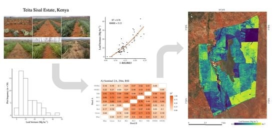
Teita Sisal Estate (3°30′S, 38°24′E, 750–900 m a.s.l) is located in the town of Mwatate in Taita-Taveta County in the Coast Province of Kenya and is right next to the Taita Hills (Figure 1). The Taita Hills are the northernmost part of the Eastern Arc Mountains, a chain of ancient mountains across the Eastern regions of Tanzania and Kenya [32,33]. The area has a semi-arid climate, where two rainy seasons occur in March to June and October to December. The long-term annual mean precipitation is 611 mm and mean temperature is 24.9 °C [34]. The main vegetation types in the nearby lowland areas are bushlands, grasslands, and riverine forests [35,36]. Small-scale farming of crops, mainly maize and beans, is also widely practiced. The soil type (Ferralsols) is characterized by deep, acidic, dark red, sandy clay soil [36]. The estate is one of the largest sisal plantations in the world and is the largest in Kenya, with a cultivable area of approximately 8851 ha. The monthly fibre production is 800 Mg on average, while the total sisal fibre production in Kenya in 1998–2019 averaged 22,975 Mg per year [7].
The following three sisal varieties are primarily cultivated at the plantation: Agave sisalana, Agave hildana, and Agave hybrid 11648, of which the latter occupies the majority of the area [37]. The crop is grown vegetatively from bulbils or suckers and the plant density at the estate is 4995 plants per hectare. Sisal is planted in double rows (two single rows next to each other) with 3.75 m spacing between double rows, 0.7 m between single rows, and 0.9 m between plants. Before planting the fields are fertilised with sisal waste produced during the fibre extraction. After the planting herbicides are applied for weed control. Management practices in subsequent years include desuckering, mowing, and bush clearing. Generally, the old blocks receive less attention than the young ones. Therefore, the younger blocks had minimal ground vegetation, while many of the older blocks had a varying cover of weeds and shrubs (Figure 2).
Sisal forms a rosette of sword-shaped (lanceolate) leaves around its stem [2,3]. Approximately 85% of the aboveground biomass (AGB) is contributed by leaves [38]. The water content of the leaves is approximately 80% and decreases with plant age [1,39]. Leaf harvesting starts at the age of 2–3 years when the oldest leaves, lowermost in the rosette, are cut manually. Harvesting continues approximately once a year up to 15 years. At the end of its life-cycle sisal grows a flower stalk up to 7 m long (Figure 2E). The leftover stump, known as sisal ball, is what remains after all the leaves and the stalk have been harvested. The sisal ball consists of a stem, bits of leaf bases, and the base of a flower stalk [11].
2.2. Field Plots and Leaf Biomass Estimation
Field plots (n = 58) were selected at Teita Sisal Estate between 22 and 29 August 2019 (Figure 1). Plot locations were chosen subjectively based on the normalized difference vegetation index (NDVI) calculated from a Sentinel-2 image (acquisition date 16 April 2019) and from prior knowledge of planting time to cover the range of plant sizes and different growing conditions. Furthermore, seven of the plots were positioned next to gas-chamber measurement sites (CO2, N2O, and CH4 fluxes were measured at these sites over a 12-month period for University of Helsinki research [40]). The 20 m2 square plots were oriented with two sides parallel to the sisal rows such that four double rows (=8 single rows) were inside the plot (Figure 3).
Plot locations were recorded with a GNSS receiver (Trimble GeoXH) by measuring the centre and the four corners of the plot. On average, the location of the centre was logged 326 times. A differential correction was applied to the measured locations in relation to a GNSS base station. The location of the base station was determined using Trimble RTX post-processing service. Plot polygons (20 m2) were then digitized in QGIS 3.4.5 using a square-drawing tool [41]. Centre location was used as the exact centre of the polygon and orientation was guided by the corner locations.
Proximity to roads was avoided and homogeneity in the plot was preferred when choosing the locations. The number of plants in the two midmost double rows was counted and multiplied by two to estimate the total number of plants in the plot. The number of leaves was counted and plant height and maximum leaf width were measured from one subjectively determined representative plant in the two midmost rows. Plant height was measured with a measurement tape from topsoil to the terminal spine of the leaf unfolding upwards from the middle of the rosette. Maximum leaf width was measured with a measurement tape along the upper surface of the leaf. The mean values of these two plants were calculated to constitute representative plot-specific plant metrics. If a considerable variance in plant sizes was visually observed, plants were then divided into two size-class categories that were measured separately. Some plots had shoots growing on the ground and they were included only if they were higher than 50 cm. Furthermore, the presence of ground vegetation and flower stalks and harvesting status were noted. Information on block age and variety was received from plantation’s books [37].
Dry leaf biomass (Mg ha−1) for the field plots was predicted using a species-specific allometric model developed by Vuorinne et al. [39]. This log-log linear model [R2 = 0.96, root mean squared error (RMSE) = 7.7g] predicts leaf mass as:
where B (Mg ha−1) is the dry mass of a leaf, W (cm) the maximum width of a leaf, and H (cm) the height of a plant. The predicted values were transformed back from the logarithmic scale to the original scale with bias correction recommended by [42]. The correction factor (CF) was calculated as:
where SE is the standard error of the regression.
log(B) = −4.12 + 0.84 log(W2H),
CF = (SE/2)2,
First, plot-specific plant metrics were used to predict the mass of a representative leaf, which was then multiplied by the number of leaves in the plant and then by the number of plants in the plot to estimate the total leaf biomass in the plot. Plot biomass varied between 0 and 42.3 Mg ha−1 (mean 12.1 Mg ha−1, Figure 4 and Table 1) and block age varied between 0 and 17 years (mean 7.5 years).
2.3. Sentinel-2 Satellite Image
A Sentinel-2 image with acquisition date 28 September 2019 was downloaded from the Copernicus Open Access Hub [43] as a level 2-A product (ID: S2B_MSIL2A_20190928T072659_N0213_R049_T37MDS_20190928T105635.SAFE). Of the cloud-free Sentinel-2 images from the study area, this was the one with the nearest date to the field data collection. Level 2-A products are analysis-ready bottom of atmosphere (BOA) reflectance images corrected with the Sen2Cor procedure [44]. The MSI (Multi-Spectral Instrument) sensor aboard Sentinel-2 satellites has 13 spectral bands with a spatial resolution of 10 to 60 m (Table 2; [45]). All bands with 20-m spatial resolution and 10-m bands down-sampled to 20-m were used in this study (B2, B3, B4, B5, B6, B7, B8A, B11, B12). Hereafter, they will be referred to as Blue, Green, Red, RE1, RE2, RE3, NIR2, SWIR1, and SWIR2.
Reflectance values for the field plots were calculated from the image by taking an area-weighted average of the pixels that fell under the plot polygon. The weights were based on pixel area that overlapped the plot polygon. The calculation was performed with a purpose-built script using Python programming language [46].
2.4. Vegetation Index Calculation
Reflectance in spectral bands can be combined into VIs with simple arithmetic to increase sensitivity to biomass [23,24]. Here the VIs were calculated using plot reflectance in all bands with 20-m spatial resolution. All possible two-band combinations were tested by using three common vegetation index formulas. These were the ratio-based spectral index (RSI):
normalised difference spectral index (NDSI):
and reciprocal difference spectral index (RDSI):
All the bands were tested as both Band A and Band B which resulted 216 band combinations altogether. In addition, a selection of published VIs were tested as references (Table 3). These included Soil Adjusted Vegetation Index (SAVI) and Enhanced Vegetation Index (EVI) which are based on NIR to Red ratio, but with additional parameters to account for atmospheric and background effects. The other indices (Canopy Chlorophyll Content Index (CCCI), Inverted Red-Edge Chlorophyll Index (IRECI) and Modified Chlorophyll Absorption Ratio Index [MCARI]) take advantage of the bands positioned in the red-edge spectral region near 700 nm [24,47]. Furthermore, widely used normalized difference vegetation index (NDVI) was used as a reference, although it was automatically included also in NDSI combinations.
2.5. Modelling Biomass with Vegetation Indices
The relationships between biomass and VIs were analysed with Generalized Additive Models (GAM) in R-Studio [53] using mgcv-package [54]. With GAMs, it is unnecessary to identify polynomial terms or predictor transformations to improve model fit. GAMs are also flexible in approximating responses and have relaxed assumptions of predictor-response relationship. Thus, they have the potential to achieve better fits than purely parametric models. In multispectral remote sensing, GAMs have been used, for example, to model leaf-area-index [55], fractional vegetation cover [56], and biomass [57]. GAM is a semiparametric generalized linear model that fits the response curves as a sum of smoothing functions [54]:
where is the response vector, is the model intercept, the smooth function, and is the residual. In GAMs, the relationship between the linear predictor and the mean of the dependent variable is provided by a link function. Here, a Gaussian-error structure was used with an identity link function. Smoothing function, which sets the upper limit on the degrees of freedom associated with the smoothing, was set to k = 3, which is considered conservative and should avoid overfitting. The models were evaluated based on deviance explained (D2), which was calculated as:
The modelling included two steps. First, GAMs were calculated for all the bands and VIs, and then, the reference VIs and two VIs with the highest D2 from each group (RS, NDSI, RDSI) were selected for further evaluation. The performance of these indices was tested with two exhaustive cross-validation methods. The leave-one-out cross-validation (LOOCV; [58]) was used first. In LOOCV, one observation at a time is left out and used as a validation set, while the model is trained with all the other observations. The process is repeated until all the observations have been used for validation, which results in a prediction size equal to the sample size. Then, mean absolute error (MAE) and RMSE were calculated between observed and predicted values. MAE as:
and RMSE as:
where y is the observed value, is the predicted value, and n is the number of observations. Normalised RMSE (nRMSE %) was calculated as:
where is the mean of the predicted biomass.
As recently demonstrated by Ploton et al. [59], cross-validations such as LOOCV can be subject to spatial autocorrelation if the observations are close to each other, leading to overoptimistic validation statistics. In a plantation environment, spatial autocorrelation should not be a similar issue as in natural environments, but some of our observation were from the same blocks, which we thought could affect LOOCV. Therefore, another validation was performed that we call leave-block-out cross-validation (LBOCV). The observations were first divided into subsets with all the observations from the same block constituting their own subset. Overall, there were observations from 30 different blocks (= 30 subsets), with 1 to 4 observations in each. We then ran a cross-validation similar to LOOCV, but instead of leaving out single observations, we left out the block subsets one at a time.
LBOCV was used also to calculate pixel-scale uncertainty for the final biomass map that was predicted using the best performing VI-biomass GAM. First, all the 30 models where one block had been left out were used to predict plantation biomass. Then standard deviation and coefficient of variation (CV, also known as relative standard error) of these predictions were calculated for all pixels [57].
3. Results
3.1. Relationship between Biomass and Vegetation Indices
Generally, biomass had an inverse relationship with Blue, Green, Red, RE1, SWIR1, and SWIR2 (Figure 5). With RE2, RE3, and NIR the relationship was positive. Although these relationships were evident, so was the variation, as there were notable spreads around the general trends. The bands that explained the most deviance in biomass were RE1, NIR, and RE3. The second best explainers were SWIR1, Red and Green while the least deviance was explained by RE2 and Blue.
Figure 6A–C shows the explained deviances (D2) of the VI-biomass GAMs fitted with all the possible two-band combinations for three VI forms (RSI, NDSI, RDSI). In all groups, the best combinations included one of the two red-edge bands (RE2, RE3) or the near-infrared band (NIR), while combinations without these bands showed lower performance. The results for RSIs and NDSIs were almost identical. The best combination of bands for both VI forms was the two red-edge bands, namely RE2/RE3 and (RE3 − RE2)/(RE3 + RE2) (D2 = 0.76). Other RE and NIR combinations also showed good performance, but the second-best combination was the G band together with either the RE3 or NIR band (NIR/Green and RE3/Green, D2 = 0.73, (NIR − Green)/(NIR + Green) and (RE3 − Green)/(RE3 + Green); D2 = 0.72). Overall, RDSIs showed lower performance than RSIs or NDSIs, although the best band combinations were similar. For RDSI, the best explanatory power was achieved with 1/RE3-1/RE1 (D2 = 0.68) and the second best with 1/RE3-/Green (D2 = 0.67).
GAMs were also fitted for all reference VIs. These models and the two best-performing RSIs, NDSIs, and RDSIs were then cross-validated using LOOCV and LBOCV methods. The LOOCV produced only slightly more optimistic statistics than LBOCV. The model fits (D2) and validation MAEs and RMSEs are presented in Table 4. Reference VIs with the best explanatory power were IRECI (D2 = 0.64) and MCARI (D2 = 0.64). However, the best RSI, NDSI, and RDSI outperformed all reference VIs. Figure 7 shows best two VIs of all the VI groups and reference VIs and NDVI and SR. Since RE2/RE3, RE3/1–RE1/1, and RE3/1–G/1 had inverse relation to biomass, they are shown as 1–VI to make the relation positive and the comparison to other models easier.
The impacts of the additional plot variables (ground vegetation, flower stalks, harvesting status, variety, and age) were analysed visually by plotting the variables with the highest performing VI (Figure 8A–E). Ground vegetation seemed to lead to overestimation in blocks with high biomass density, although there were a few observations contradicting this trend (Figure 8A). Conversely, in the lower densities, biomass was generally underestimated for the blocks without ground vegetation. Furthermore, low density blocks that had not yet been harvested had greater prediction error than those that had been harvested (Figure 8C). Flower stalks, variety, or age did not seem to introduce notable error trends (Figure 8C–E).
3.2. Biomass Map
The best performing model (RE2/RE3) was used to predict leaf biomass at the plantation level (Figure 9). Since the identity link function in GAM allows the model to predict negative values, they were set to 0. Biomass densities ranged from 0 to 46.7 Mg ha−1 (mean biomass 10.6 Mg ha−1) and the total biomass at the plantation was 94,044 Mg. There was large intra- and inter-block variation in biomass. Primarily, the age of a block and leaf harvesting controlled the biomass. The lowest densities were found from recently planted blocks, while the densities of the mature and old blocks where harvesting had begun were close to the plantation mean. The highest densities were found from 2- to 4-year-old blocks, where leaves had not yet been harvested or the harvesting had just begun. The areas with no biomass were recently ploughed blocks.
Many of the blocks appeared internally heterogeneous. For example, the block with high biomass density in the middle of eastern edge of the plantation had randomly distributed spots with lower density, indicating possible disturbances. Furthermore, there were regular north-south oriented line-shaped spatial patterns that were almost perpendicular to the crop rows, indicating more rigorous growth in some parts of the block.
The uncertainty maps are presented in Figure 10. Pixel-scale standard deviation was generally low, except in the blocks with the highest biomass densities. Conversely, CV was the highest in the fields with low biomass, especially in the blocks that had just been planted. Hence, the stability of the predictions was lowest in high density blocks in terms of actual biomass quantities and in low density blocks relative to the amount of biomass.
4. Discussion
Although remote sensing can be a feasible method for a large-scale assessment and monitoring of crop biomass, the methods and outcomes are often species specific. The objective of this study was to assess the utility of Sentinel-2 imagery in estimating leaf biomass of Agave sisalana. The results show a strong relationship between multispectral vegetation indices and biomass. The best results were achieved with ratio and normalised difference VIs and the most valuable single bands were RE2, RE3, and NIR, but also Green. The two best ratio indices appear to be similar to Red-edge Chlorophyll Index (CIRE) and Green Chlorophyll Index (CIGreen), while the normalised difference ratio indices are similar to Green NDVI (GNDVI) and Red-Edge NDVI (NDVIre), all of which Gitelson and Merzlyak [24] and Gitelson et al. [25,60] revealed were sensitive to LAI and green-leaf biomass at the leaf and canopy level. The applicability of these indices for crop studies using Sentinel-2 data have also been demonstrated before [23].
The distinctive feature of the RE indices that showed the highest sensitivity to sisal leaf biomass is that even though they are broadly based on the same spectral regions as in previous crop studies, they were calculated using bands with slightly different positioning. Originally, CIRE, and NDVIRE were formulated using narrow spectral bands (1 nm) as 750/700 nm and (750 − 700 nm)/(750 − 700 nm), respectively [24,60]. Hence, when calculated from multispectral data, the band corresponding to NIR has usually been used as numerator and the band nearest to 700 nm as denominator. For example, Kross et al. [29] calculated NDVIRE using RapidEye NIR (760–850 nm) and RE (690–730 nm) bands, when estimating the LAI and biomass of corn and soybean. Using Sentinel-2 data, Clevers et al. [23] calculated CIRE using RE3 (773–793 nm) and RE1 (698–713 nm) for retrieving chlorophyll and LAI of potato. Here, the best performing RE indices were calculated using RE2 (733–748 nm) and RE3 (773–793 nm). Using RE2 instead of the band closest to 700 nm (as in other crop studies) increased the explained deviance by 9.3% at best.
The functioning of the red-edge indices is based on the premise that the red-edge position (the point of the maximum slope between red and NIR wavelengths) is mainly controlled by chlorophyll content, shifting to higher wavelengths with increasing chlorophyll [47]. Therefore, it can provide information about various plant parameters. It is known that the reflectance near 700 nm is a sensitive indicator of the red-edge position and, furthermore, that the ratio of 750 nm to that near 700 nm is directly proportional to chlorophyll content and green-leaf biomass [60]. However, these relationships were originally observed for maize with leaf biomass of 0 to 3.5 Mg ha−1, while sisal leaf biomass in the study area ranged from 0 to 46.7 Mg ha−1, with the mean at 10.6 Mg ha−1. Structural differences between these crops at the leaf and canopy level are also prominent. Presumably, due to higher biomass quantities and the consequent expansion of chlorophyll concentration, the sisal RE position can move to longer wavelengths than that of maize. This is supported with two indicative observations. Firstly, the RE1 band centred at 705 nm had a negative relation to biomass, resembling a spectral response that healthy plants generally exhibit on the red band. Secondly, the ratio (RE2/RE3) that was most sensitive to sisal leaf biomass was calculated from longer wavelengths than those that have optimal sensitivity for maize biomass [59].
Relatively high biomass densities and sisal structure also likely explain why reference VIs, all of which included the Red band, had weaker sensitivity to biomass. Although NIR/Red ratios are known to correlate with biomass, they tend to saturate at high densities [27]. This is because at red wavelengths, the absorption coefficient of chlorophylls is high and the depth of light penetration into the leaf is low [61,62]. In contrast, sisal has thick pulpy leaves with high water content, multiple leaf layers (and consequently a high amount of green biomass) [2,3], and high chlorophyll content. This is likely to explain why the Red band showed low sensitivity to biomass. In addition to the Red band, the best reference VI (IRECI) contained also the RE bands, whereas reference VIs based solely on the NIR and R bands, such as NDVI, showed lower performance.
In addition to the NIR and RE bands, the Green band also showed good sensitivity to biomass. A strong relationship, almost as strong as for RE indices, was observed for NIR/Green and (NIR-Green)/(NIR+Green), known as ClGreen and GNDVI [24,25]. These indices also appeared to be slightly more sensitive to lower biomass values than the RE indices. Just like the red-edge position, the reflectance at the green spectral region is controlled by chlorophyll content. In this region, the absorption coefficient of chlorophyll is smaller and light can penetrate deeper into the leaf than at the red region [61,62]. Therefore, the green region does not saturate as easily and is highly sensitive to changes in chlorophyll content [24,25]. Although the NIR/red combinations have been the preferred option in vegetation studies, Gitelson et al. [25] have advocated the use of NIR/green combinations due to the wider dynamic range of the green bands. Clevers et al. [23] have also found ClGreen to be a better indicator of potato canopy chlorophyll content than CIRE. In Sentinel-2, the G band is available at 10-m resolution, whereas the RE bands are available only at 20-m resolution. Hence NIR/Green can be calculated at higher resolution, although this does not necessarily boost the model performance [56]. Furthermore, unlike the red-edge bands, the NIR and Green bands are found from all multispectral satellites, which makes this combination more available and interoperable with other optical sensors.
One challenge of the VI-modelling approach is how to minimize the impact of external factors and to establish a truly sensitive relationship between VIs and biomass [13,30]. In terms of model fit, the performance of the best models in this study appear to be slightly lower than in other studies that have used multispectral data for crop biomass assessment. For example, Kross et al. [29] achieved a coefficient of determination (R2) ranging between 0.86 and 0.88 when mapping corn and soybean biomass with RapidEye imagery. Prabhakara et al. achieved an R2 of 0.86 for six winter crops with a handheld multispectral spectrometer [31]. For wheat biomass assessment, Wang et al. used an HJ1 satellite data that yielded an R2 of 0.79 [18]. Then again, for biomass assessment of rangeland grasses with Sentinel-2, Sibanda et al. achieved R2 of 0.58 [22].
Compared to the crops in the studies mentioned above (soybean, corn, wheat), which grow in more homogeneous fields, the growing conditions of sisal in the study area were rather different. Although this was a monoculture plantation, the varying management practices yielded blocks that were heterogeneous in terms of ground vegetation between the crop rows (Figure 2). Some blocks had no or a minimal number of weeds, while in other blocks the 3.75-m space between the sisal rows was fully covered with tall grass or shrubs, or both. In older blocks, tall (up to 10 m) acacia trees also grew among sisal. With Sentinel’s 20-m resolution, this means that the signal is always a mixture of sisal and either soil, trees or ground vegetation, or all. Spectral regions used in the red-edge and NIR to G ratios, which showed the best sensitivity to biomass, have exhibited low sensitivity to soil background effects [63,64]. However, it should be acknowledged that the sensitivity of VIs to soil depends on the soil type and wider evaluation of soil-adjusted indices could therefore be relevant [65]. The CV map also showed that the prediction stability was low in recently planted fields, meaning that the models omitting observations from these fields had large error for such fields. Ground vegetation also seemed to introduce uncertainties in the models with an over- or under-prediction trend depending on the biomass density. Hence, also the effects of ground vegetation should be analysed further. Overall, the background effects could be studied, for example, by stratifying the observations based on the growing conditions (e.g., the abundance of ground vegetation).
Even though the acquisition date of the Sentinel-2 image was a month apart from the fieldwork, changes in ground vegetation were presumably small, since both the fieldwork and image acquisition dates were in the middle of the dry season. Over a year, however, the seasonality of the rains and resulting phenological patterns cause the ground vegetation to change both in abundance and colour. If ground vegetation causes bias as speculated, the models may potentially perform poorer during the rainy season due to the greening of herbaceous vegetation [66,67]. This study covered for wide range of plant ages and growing conditions but only in one area at one point in time. The generalisation of results in space and time is therefore constrained, because of factors arising from sensor variations and changes in biotic and abiotic conditions [68]. Further research is needed to see how the relationship between sisal leaf biomass and VIs varies between sensors, in different regions, and over time.
The 1-month gap between the fieldwork dates and the acquisition date of the nearest fully cloud-free Sentinel-2 image of the study area demonstrates one shortcoming of the optical satellites. In areas with regular cloud cover, the potential benefits of the frequent revisit time (less than one week for Sentinel-2) of multispectral satellites can seldom be realized [69]. This makes the availability of data unpredictable and hampers the possibility of frequent monitoring. The use of complementary data sources such as radar, which are not affected by cloud cover, should be studied. Combined with multispectral data, SAR could also enhance the model accuracy [66]. Another potential complementary or alternative data source for biomass modelling is UAVs [70] or airborne remote sensing [71]. With UAVs or other data sources with comparable spatial resolution, the background effects could probably be diminished, since earlier research has demonstrated the possibility of separating Agave rows from weeds using fine-resolution data [72]. Furthermore, with airborne and UAV remote sensing, data acquisition can be scheduled according to phenology and weather [73].
The study area consisted of field blocks at different stages of the growing cycle. The resultant map revealed that with 20-m resolution, the variations in biomass densities can be detected not only across the plantation but also inside the blocks, since many of them were internally heterogeneous. In addition, during fieldwork it was observed that in the older fields some of the plants had been fully harvested, while others still had leaves. In the biomass map, such areas exhibited irregular spatial patterns. Furthermore, the map had regular patterns indicating better growth in some areas, probably due to edaphic factors such as favourable soil moisture or nutrients. These observations indicate that the resolution would be sufficient for monitoring the growth and detecting disturbances in individual blocks at sisal or other Agave plantations. By using the NIR to Green ratio, the map can be produced at 10-m resolution, adding even more detail to the analysis.
Sisal plantations are an established land-use type in East Africa and in other tropical and subtropical regions [7]. This study showed how multispectral satellite data can be applied to retrieve the leaf biomass of sisal in a plantation environment. This is beneficial for agricultural management, since this offers the means to assess resources and monitor growth remotely over large areas. In addition to sisal, other Agaves grown at commercial plantations, such as for the beverage and sweetener industries in Central America, also have great economic importance [4]. This study paves the way for the use of multispectral remote sensing for obtaining crop information at Agave plantations for precision agriculture.
5. Conclusions
In this study, Sentinel-2 vegetation indices were tested for mapping Agave sisalana leaf biomass in a plantation environment. The best results were achieved with indices based on the green (R560), red-edge (R740 and R783), and near-infrared (R865) bands, which resulted in explained deviance = 76% and RMSE = 5.15 Mg ha−1 (49% of the mean) at best. These results demonstrate the effectiveness of medium resolution multispectral satellite data for modelling sisal leaf biomass. Such crop information can be used for agricultural monitoring and to study carbon cycling at sisal plantations. Because cloud cover affects the availability of such data, complementary data sources should be investigated. Furthermore, since varying ground vegetation seems to introduce uncertainties to the models, the accuracies could be increased by studying the background effects. Finally, further study is recommended to assess the relationships between sisal biomass and vegetation indices in other areas and between years and seasons.
Author Contributions
Conceptualization, I.V., J.H. and P.K.E.P.; methodology, I.V., J.H.; software, I.V.; validation, I.V., formal analysis, I.V.; investigation, I.V. and J.H.; resources, I.V., J.H. and P.K.E.P.; data curation, I.V.; writing—original draft preparation, I.V.; writing—review and editing, I.V., J.H. and P.K.E.P.; visualization, I.V.; supervision, J.H. and P.K.E.P.; project administration, P.K.E.P., funding acquisition, P.K.E.P. All authors have read and agreed to the published version of the manuscript.
Funding
This research was funded by the Academy of Finland (Environmental sensing of ecosystem services for developing a climate-smart landscape framework to improve food security in East Africa, SMARTLAND decision no. 318645).
Institutional Review Board Statement
Not applicable.
Informed Consent Statement
Not applicable.
Data Availability Statement
The data presented in this study are available on request from the author (I.V.).
Acknowledgments
We would like to thank Taita Taveta University for logistical support. We gratefully acknowledge the support provided by the Teita Sisal Estate, namely Emmanuel Mrombo. The Taita Research Station of the University of Helsinki is acknowledged for logistical support. We sincerely thank Mwadime Mjomba and Darius Kimuzi for assistance in the field and Niklas Sädekoski from the University of Helsinki. Research permission from NACOSTI (no. P/18/97336/26355) is acknowledged. Finally, we are thankful for five anonymous reviewers for their valuable comments on our manuscript.
Conflicts of Interest
The authors declare no conflict of interest.
References
- Sataya, B.; Maiti, R. Bast and Leaf Fibre Crops: Kenaf, Hemp, Jute, Agave, etc. In Biofuel Crops: Production, Physiology and Genetics; Singh, B.P., Ed.; CABI: Oxfordshire, UK, 2013; pp. 292–308. [Google Scholar] [CrossRef]
- Davis, S.C.; Stephen, P.L. Sisal/Agave. In Industrial Crops: Breeding for Bioenergy and Bioproducts; Von Cruz, M.V., Dierig, D.A., Eds.; Springer Nature: Berlin/Heidelberg, Germany, 2015; pp. 339–345. [Google Scholar] [CrossRef]
- Blunden, G.; Yi, Y.; Jewers, K. The comparative leaf anatomy of Agave, Beschorneria, Doryanthes and Furcraea species (Agavaceae: Agaveae). Bot. J. Linn. Soc. 1973, 66, 157–179. [Google Scholar] [CrossRef]
- Stewart, J.R. Agave as a model CAM crop system for a warming and drying world. Front. Plant Sci. 2015, 6, 684. [Google Scholar] [CrossRef] [PubMed] [Green Version]
- Sahu, P.; Gupta, M.K. Sisal (Agave sisalana) fibre and its polymer-based composites: A review on current developments. J. Reinf. Plast. Compos. 2017, 36, 1759–1780. [Google Scholar] [CrossRef]
- Santos, J.D.G.; Vieira, I.J.C.; Braz-Filho, R.; Branco, A. Chemicals from Agave sisalana Biomass: Isolation and Identification. Int. J. Mol. Sci. 2015, 16, 8761–8771. [Google Scholar] [CrossRef] [PubMed] [Green Version]
- Food and Agriculture Organisation of the United Nations, FAOSTATS. Available online: http://www.fao.org/faostat/en/#data/QC (accessed on 22 September 2020).
- Davis, S.C.; Dohleman, F.G.; Long, S.P. The global potential for Agave as a biofuel feedstock. Glob. Change Biol. Bioenergy 2011, 3, 68–78. [Google Scholar] [CrossRef]
- Niechayev, N.A.; Jones, A.M.; Rosenthal, D.M.; Davis, S.C. A model of environmental limitations on production of Agave americana L. grown as a biofuel crop in semi-arid regions. J. Exp. Bot. 2019, 70, 6549–6559. [Google Scholar] [CrossRef]
- Pérez-Pimienta, J.A.; López-Ortega, M.G.; Sanchez, A. Recent developments in Agave performance as a drought-tolerant biofuel feedstock: Agronomics, characterization, and biorefining. Biofuels Bioprod. Biorefining 2017, 11, 732–748. [Google Scholar] [CrossRef]
- Terrapon-Pfaff, J.C.; Fischedick, M.; Monheim, H. Energy potentials and sustainability—The case of sisal residues in Tanzania. Energy Sustain. Dev. 2012, 16, 312–319. [Google Scholar] [CrossRef] [Green Version]
- Nobel, P.S.; García-moya, E.; Quero, E. High annual productivity of certain agaves and cacti under cultivation. Plant Cell Environ. 1992, 329–335. [Google Scholar] [CrossRef]
- Weiss, M.; Jacob, F.; Duveiller, G. Remote sensing for agricultural applications: A meta-review. Remote Sens. Environ. 2020, 236, 111402. [Google Scholar] [CrossRef]
- Battude, M.; Al Bitar, A.; Morin, D.; Cros, J.; Huc, M.; Sicre, C.M.; Le Dantec, V.; Demarez, V. Estimating maize biomass and yield over large areas using high spatial and temporal resolution Sentinel-2 like remote sensing data. Remote Sens. Environ. 2016, 184, 668–681. [Google Scholar] [CrossRef]
- Gao, F.; Anderson, M.C.; Zhang, X.; Yang, Z.; Alfieri, J.G.; Kustas, W.P.; Mueller, R.; Johnson, D.M.; Prueger, J.H. Toward mapping crop progress at field scales through fusion of Landsat and MODIS imagery. Remote Sens. Environ. 2017, 188, 9–25. [Google Scholar] [CrossRef] [Green Version]
- Kanke, Y.; Tubaña, B.; Dalen, M.; Harrell, D. Evaluation of red and red-edge reflectance-based vegetation indices for rice biomass and grain yield prediction models in paddy fields. Precis. Agric. 2016, 17, 507–530. [Google Scholar] [CrossRef]
- Serrano, L.; Filella, L.; Penuelas, J. Remote Sensing of Biomass and Yield of Winter Wheat. Crop. Sci. 2000, 40, 723–731. [Google Scholar] [CrossRef] [Green Version]
- Wang, L.; Zhou, X.; Zhu, X.; Dong, Z.; Guo, W. Estimation of biomass in wheat using random forest regression algorithm and remote sensing data. Crop. J. 2016, 4, 212–219. [Google Scholar] [CrossRef] [Green Version]
- Lemus, R.; Lal, R. Bioenergy crops and carbon sequestration. Crit. Rev. Plant Sci. 2005, 24, 1–21. [Google Scholar] [CrossRef]
- Mathew, I.; Shimelis, H.; Mutema, M.; Chaplot, V. What crop type for atmospheric carbon sequestration: Results from a global data analysis. Agric. Ecosyst. Environ. 2017, 243, 34–46. [Google Scholar] [CrossRef]
- Castillo, J.A.A.; Apan, A.A.; Maraseni, T.N.; Salmo, S.G. Estimation and mapping of above-ground biomass of mangrove forests and their replacement land uses in the Philippines using Sentinel imagery. ISPRS J. Photogramm. Remote Sens. 2017, 134, 70–85. [Google Scholar] [CrossRef]
- Sibanda, M.; Mutanga, O.; Rouget, M. Examining the potential of Sentinel-2 MSI spectral resolution in quantifying above ground biomass across different fertilizer treatments. ISPRS J. Photogramm. Remote Sens. 2015, 110, 55–65. [Google Scholar] [CrossRef]
- Clevers, J.G.P.W.; Kooistra, L.; van den Brande, M.M.M. Using Sentinel-2 data for retrieving LAI and leaf and canopy chlorophyll content of a potato crop. Remote Sens. 2017, 9, 405. [Google Scholar] [CrossRef] [Green Version]
- Gitelson, A.; Merzlyak, M.N. Spectral Reflectance Changes Associated with Autumn Senescence of Aesculus hippocastanum L. and Acer platanoides L. Leaves. Spectral Features and Relation to Chlorophyll Estimation. J. Plant. Physiol. 1994, 143, 286–292. [Google Scholar] [CrossRef]
- Gitelson, A.A.; Kaufman, Y.J.; Merzlyak, M.N. Use of a green channel in remote sensing of global vegetation from EOS-MODIS. Remote Sens. Environ. 1996, 58, 289–298. [Google Scholar] [CrossRef]
- Frampton, W.J.; Dash, J.; Watmough, G.; Milton, E.J. Evaluating the capabilities of Sentinel-2 for quantitative estimation of biophysical variables in vegetation. ISPRS J. Photogramm. Remote Sens. 2013, 82, 82–92. [Google Scholar] [CrossRef] [Green Version]
- Mutanga, O.; Skidmore, A.K. Narrow band vegetation indices overcome the saturation problem in biomass estimation. Int. J. Remote Sens. 2004, 25, 3999–4014. [Google Scholar] [CrossRef]
- Revill, A.; Florence, A.; MacArthur, A.; Hoad, S.P.; Rees, R.M.; Williams, M. The value of Sentinel-2 spectral bands for the assessment of winter wheat growth and development. Remote Sens. 2019, 11, 2050. [Google Scholar] [CrossRef] [Green Version]
- Kross, A.; McNairn, H.; Lapen, D.; Sunohara, M.; Champagne, C. Assessment of RapidEye vegetation indices for estimation of leaf area index and biomass in corn and soybean crops. Int. J. Appl. Earth Obs. Geoinf. 2015, 34. [Google Scholar] [CrossRef] [Green Version]
- Marshall, M.; Thenkabail, P. Advantage of hyperspectral EO-1 Hyperion over multispectral IKONOS, GeoEye-1, WorldView-2, Landsat ETM+, and MODIS vegetation indices in crop biomass estimation. ISPRS J. Photogramm. Remote Sens. 2015, 108, 205–218. [Google Scholar] [CrossRef] [Green Version]
- Prabhakara, K.; Hively, W.D.; McCarty, G.W. Evaluating the relationship between biomass, percent groundcover and remote sensing indices across six winter cover crop fields in Maryland, United States. Int. J. Appl. Earth Obs. Geoinf. 2015, 39, 88–102. [Google Scholar] [CrossRef] [Green Version]
- Pellikka, P.K.E.; Clark, B.J.F.; Gosa, A.G.; Himberg, N.; Hurskainen, P.; Maeda, E.; Mwang’ombe, J.; Omoro, L.M.A.; Siljander, M. Agricultural Expansion and Its Consequences in the Taita Hills, Kenya. Dev. Earth Surf. Process. 2013, 16, 165–179. [Google Scholar] [CrossRef] [Green Version]
- Platts, P.J.; Burgess, N.D.; Gereau, R.E.; Lovett, J.C.; Marshall, A.R.; McClean, C.J.; Pellikka, P.K.E.; Swetnam, R.D.; Marchant, R. Delimiting tropical mountain ecoregions for conservation. Environ. Conserv. 2011, 38, 312–324. [Google Scholar] [CrossRef] [Green Version]
- Fick, S.E.; Hijmans, R.J. WorldClim 2: New 1-km spatial resolution climate surfaces for global land areas. Int. J. Climatol. 2017, 37, 4302–4315. [Google Scholar] [CrossRef]
- Pellikka, P.K.E.; Heikinheimo, V.; Hietanen, J.; Schäfer, E.; Siljander, M.; Heiskanen, J. Impact of land cover change on aboveground carbon stocks in Afromontane landscape in Kenya. Appl. Geogr. 2018, 94, 178–189. [Google Scholar] [CrossRef]
- Wachiye, S.; Merbold, L.; Vesala, T.; Rinne, J.; Räsänen, M.; Leitner, S.; Pellikka, P.K.E. Soil Greenhouse Gas Emissions under Different Land-Use Types in Savanna Ecosystems of Kenya. Biogeosciences 2019, 17, 2149–2167. [Google Scholar] [CrossRef] [Green Version]
- Mrombo, E.; Teita Sisal Estate, Taita-Taveta, Kenya. Personal communication, 2019.
- Nobel, P.S. Par, Water, and Temperature Limitations on the Productivity of Cultivated Agave fourcroydes (Henequen). J. Appl. Ecol. 1985, 157–173. [Google Scholar] [CrossRef]
- Vuorinne, I.; Heiskanen, J.; Mwangala, L.; Maghenda, M.; Pellikka, P. Estimating Agave Sisalana Leaf Biomass and Productivity in a Semi-arid Environment. (under review).
- Wachiye, S.; Merbold, L.; Vesala, T.; Rinne, J.; Leitner, S.; Räsänen, M.; Vuorinne, I.; Heiskanen, J.; Pellikka, P. Soil Greenhouse Gas Emissions from a Sisal Chronosequence in Kenya. (under review).
- QGIS Development Team. QGIS Geographic Information System. Open Source Geospatial Foundation. 2019. Available online: http://qgis.org (accessed on 1 November 2019).
- Baskerville, G.L. Use of Logarithmic Regression in the Estimation of Plant Biomass: Reply. Can. J. For. Res. 1974, 4, 149. [Google Scholar] [CrossRef]
- Copernicus Open Access Hub. Available online: https://scihub.copernicus (accessed on 1 November 2019).
- Sen2Cor Configuration and User Manual. Available online: http://step.esa.int/thirdparties/sen2cor/2.8.0/docs/S2-PDGS-MPC-L2A-SUM-V2.8.pdf (accessed on 28 December 2020).
- Sentinel-2 User Handbook. Available online: https://sentinels.copernicus.eu/documents/247904/685211/Sentinel-2_User_Handbook (accessed on 1 April 2020).
- Python Software Foundation. Python Language Reference, Version 3.6. Available online: http://www.python.org (accessed on 1 April 2020).
- Horler, D.N.H.; Dockray, M.; Barber, J. The red edge of plant leaf reflectance. Int. J. Remote Sens. 1983, 4, 273–288. [Google Scholar] [CrossRef]
- Rondeaux, G.; Steven, M.; Baret, F. Optimization of soil-adjusted vegetation indices. Remote Sens. Environ. 1996, 55, 95–107. [Google Scholar] [CrossRef]
- Huete, A.; Didan, J.; Miura, T.; Rodriguez, E.P.; Gao, X.; Ferreira, L.G. Overview of the radiometric and biophysical performance of the MODIS vegetation indices. Remote Sens. Environ. 2002, 83, 195–213. [Google Scholar] [CrossRef]
- Barnes, E.M.; Clarke, T.R.; Richards, S.E.; Colaizzi, P.D.; Haberland, J.; Kostrzewski, M.; Waller, P.; Choi, C.R.E.; Thompson, T.; Lascano, R.J.; et al. Coincident detection of crop water stress, nitrogen status and canopy density using ground based multispectral data. In Proceedings of the 5th International Conference on Precision Agriculture, Bloomington, MN, USA, 16–19 July 2000. [Google Scholar]
- Daughtry, C.S.T.; Walthall, C.L.; Kim, M.S.; De Colstoun, E.B.; McMurtrey, J.E. Estimating corn leaf chlorophyll concentration from leaf and canopy reflectance. Remote Sens. Environ. 2000, 74, 229–239. [Google Scholar] [CrossRef]
- Rouse, W.; Haas, R.H.; Deering, D.W. Monitoring Vegetation Systems in the Great Plains with ERTS. Available online: https://ntrs.nasa.gov/citations/19740022614 (accessed on 1 April 2020).
- R Core Team. R: A Language and Environment for Statistical Computing; Version 3.4.0; R Foundation for Statistical Computing: Vienna, Austria, 2020. [Google Scholar]
- Wood, S.N. Generalized Additive Models: An Introduction with R, 2nd ed.; Taylor & Francis: New York, NY, USA, 2017. [Google Scholar] [CrossRef]
- Korhonen, L.; Hadi; Packalen, P.; Rautiainen, M. Comparison of Sentinel-2 and Landsat 8 in the estimation of boreal forest canopy cover and leaf area index. Remote Sens. Environ. 2017, 195, 259–274. [Google Scholar] [CrossRef]
- Riihimäki, H.; Luoto, M.; Heiskanen, J. Estimating fractional cover of tundra vegetation at multiple scales using unmanned aerial systems and optical satellite data. Remote Sens. Environ. 2019, 224, 119–132. [Google Scholar] [CrossRef]
- Fassnacht, F.E.; Poblete-Olivares, J.; Rivero, L.; Lopatin, J.; Ceballos-Comisso, A.; Galleguillos, M. Using Sentinel-2 and canopy height models to derive a landscape-level biomass map covering multiple vegetation types. Int. J. Appl. Earth Obs. Geoinf. 2021, 94, 102236. [Google Scholar] [CrossRef]
- Ruppert, D. The Elements of Statistical Learning: Data Mining, Inference, and Prediction. J. Am. Stat. Assoc. 2004, 99, 567. [Google Scholar] [CrossRef]
- Ploton, P.; Mortier, F.; Réjou-Méchain, M.; Barbier, N.; Picard, N.; Rossi, V.; Dormann, C.; Cornu, G.; Viennois, G.; Bayol, N.; et al. Spatial validation reveals poor predictive performance of large-scale ecological mapping models. Nat. Commun. 2020, 11, 4540. [Google Scholar] [CrossRef] [PubMed]
- Gitelson, A.A.; Viña, A.; Arkebauer, T.J.; Runquist, D.C.; Keydan, G.; Leavitt, B. Remote Estimation of green leaf biomass in maize canopies. Geophys. Res. Lett. 2003, 30, 1248. [Google Scholar] [CrossRef] [Green Version]
- Kumar, R.; Silva, L. Light Ray Tracing Through a Leaf Cross Section. Appl. Opt. 1973, 12, 2950–2954. [Google Scholar] [CrossRef]
- Lichtenthaler, H.K. Chlorophylls and Carotenoids: Pigments of Photosynthetic Biomembranes. Methods Enzymol. 1987, 148, 350–382. [Google Scholar] [CrossRef]
- Prudnikova, E.; Savin, I.; Vindeker, G.; Grubina, P.; Shishkonakova, E.; Sharychev, D. Influence of soil background on spectral reflectance of winter wheat crop canopy. Remote Sens. 2019, 11, 1932. [Google Scholar] [CrossRef] [Green Version]
- Viña, A.; Gitelson, A.A.; Nguy-Robertson, A.L.; Peng, Y. Comparison of different vegetation indices for the remote assessment of green leaf area index of crops. Remote Sens. Environ. 2011, 115, 3468–3478. [Google Scholar] [CrossRef]
- Darvishzadeh, R.; Skidmore, A.; Atzberger, C.; van Wieren, S. Estimation of vegetation LAI from hyperspectral reflectance data: Effects of soil type and plant architecture. Int. J. Appl. Earth Obs. Geoinf. 2008, 10, 358–373. [Google Scholar] [CrossRef]
- Forkuor, G.; Zoungrana, J.B.B.; Dimobe, K.; Ouattara, B.; Vadrevu, K.P.; Tondoh, J.E. Above-ground biomass mapping in West African dryland forest using Sentinel-1 and 2 datasets—A case study. Remote Sens. Environ. 2020, 235, 111496. [Google Scholar] [CrossRef]
- Liu, J.; Heiskanen, J.; Aynekulu, E.; Maeda, E.E.; Pellikka, P.K.E. Land cover characterization in West Sudanian savannas using seasonal features from annual landsat time series. Remote Sens. 2016, 8, 365. [Google Scholar] [CrossRef] [Green Version]
- Foody, G.M.; Boyd, D.S.; Cutler, M.E.J. Predictive relations of tropical forest biomass from Landsat TM data and their transferability between regions. Remote Sens. Environ. 2003, 85, 463–474. [Google Scholar] [CrossRef]
- Asner, G.P. Cloud cover in Landsat observations of the Brazilian Amazon. Int. J. Remote Sens. 2001, 22, 3855–3862. [Google Scholar] [CrossRef]
- Han, L.; Yang, G.; Dai, H.; Xu, B.; Yang, H.; Feng, H.; Li, Z.; Yang, X. Modeling maize above-ground biomass based on machine learning approaches using UAV remote-sensing data. Plant Methods 2019, 15. [Google Scholar] [CrossRef] [Green Version]
- Piiroinen, R.; Heiskanen, J.; Mõttus, M.; Pellikka, P.K.E. Classification of crops across heterogeneous agricultural landscape in Kenya using AisaEAGLE imaging spectroscopy data. Int. J. Appl. Earth Obs. Geoinf. 2015, 39, 1–8. [Google Scholar] [CrossRef]
- Calvario, G.; Sierra, B.; Alarcón, T.E.; Hernandez, C.; Dalmau, O. A multi-disciplinary approach to remote sensing through low-cost UAVs. Sensors 2017, 17, 1411. [Google Scholar] [CrossRef] [Green Version]
- Landmann, T.; Piiroinen, R.; Makori, D.M.; Abdel-Rahman, E.M.; Makau, S.; Pellikka, P.K.E.; Raina, S.K. Application of hyperspectral remote sensing for flower mapping in African savannas. Remote Sens. Environ. 2015, 166, 50–60. [Google Scholar] [CrossRef]
Figure 1.
Map of the study area (Teita Sisal Estate). Sentinel-2 true-colour image from 28 September 2019 as a base map.
Figure 1.
Map of the study area (Teita Sisal Estate). Sentinel-2 true-colour image from 28 September 2019 as a base map.

Figure 2.
Images from the study area (Teita Sisal Estate). (A) Sisal suckers ready to be planted. (B) 1-year-old block with minimal ground vegetation. (C) 3-year-old block with no ground vegetation. (D) 7-year-old block and dry weeds. (E) 13-year-old block at the end of flowering stage and with minimal ground vegetation. (F) Old field, where weeds have taken over.

Figure 3.
Schematic of the plot design for field estimation of biomass.

Figure 4.
Histogram showing the distribution of the biomass in the field plots. Bin width = 5 Mg ha−1.
Figure 4.
Histogram showing the distribution of the biomass in the field plots. Bin width = 5 Mg ha−1.

Figure 5.
The relationship between Sentinel-2 spectral bands (surface reflectance, 0–1) and sisal leaf biomass. Subfigures (A–I) show the relationship all 20-m bands.
Figure 5.
The relationship between Sentinel-2 spectral bands (surface reflectance, 0–1) and sisal leaf biomass. Subfigures (A–I) show the relationship all 20-m bands.

Figure 6.
Explained deviances (D2) of GAMs fitted with all Sentinel-2 two-band combinations. (A) Ratio-based spectral indices (RSI = Band A/Band B). (B) Normalised difference spectral indices ((NDSI = Band A − Band B)/(Band A + Band B)). (C) Reciprocal difference spectral indices (RDSI = 1/Band A − 1/Band B).

Figure 7.
Best performing biomass-VI GAMs (orange line) from ratio (A,C), normalised difference (B,D) reciprocal difference (E,F), and reference groups (G,H). NDVI (I) as reference is included. D2 = deviance explained. RMSE = root mean squared error (Mg ha−1), based on leave-block-out cross-validation. In panels A, E, and F, the VIs are shown as 1–VI to make the relation to biomass positive.

Figure 8.
The best VI-biomass model (RE2/RE3), with observations coloured based on additional plot variables. (A) Presence of ground vegetation. (B) Flower stalks. (C) Harvesting status. (D) Sisal variety. (E) Block age.
Figure 8.
The best VI-biomass model (RE2/RE3), with observations coloured based on additional plot variables. (A) Presence of ground vegetation. (B) Flower stalks. (C) Harvesting status. (D) Sisal variety. (E) Block age.

Figure 9.
Sisal leaf biomass in the study area (29 September 2019).

Figure 10.
Sisal leaf biomass pixel-scale standard deviation and coefficient of variation of leave-block-out cross-validation.
Figure 10.
Sisal leaf biomass pixel-scale standard deviation and coefficient of variation of leave-block-out cross-validation.


Table 1.
Summary of the field plot biomass.
| Min. | 1st. Quantile | Median | Mean | 3rd. Quantile | Max. | |
|---|---|---|---|---|---|---|
| Leaf Biomass (Mg ha−1) | 0.0 | 5.1 | 10.0 | 12.1 | 16.0 | 42.3 |
| Block Age (years) | 0 | 3 | 7 | 7.5 | 13 | 17 |
Table 2.
Sentinel-2 spectral bands.
| Band | Spectral Band | Central Wavelength (nm) | Band Width (nm) | Spatial Resolution |
|---|---|---|---|---|
| B1 | Coastal aerosol | 443 | 20 | 60 |
| B2 | Blue | 490 | 65 | 10 |
| B3 | Green | 560 | 35 | 10 |
| B4 | Red | 665 | 30 | 10 |
| B5 | Red-edge, RE1 | 705 | 15 | 20 |
| B6 | Red-edge, RE2 | 740 | 15 | 20 |
| B7 | Red-edge, RE3 | 783 | 20 | 20 |
| B8 | Near infrared | 842 | 115 | 10 |
| B8A | Near infrared narrow, NIR | 865 | 20 | 20 |
| B9 | Water vapour | 945 | 20 | 60 |
| B10 | Shortwave infrared | 1380 | 30 | 60 |
| B11 | Shortwave infrared, SWIR1 | 1910 | 90 | 20 |
| B12 | Shortwave infrared, SWIR2 | 2190 | 180 | 20 |
Table 3.
Vegetation indices used as a reference.
| Index | Formula | Reference |
|---|---|---|
| SAVI | ((NIR − Red))/((NIR + Red + 0.16)) | [48] |
| EVI | 2.5 × (NIR − Red)/((NIR + 6Red − 7.5Blue) + 1) | [49] |
| CCCI | ((NIR − RE1)/(NIR + RE1))/((NIR − Red)/(NIR+Red)) | [50] |
| IRECI | (NIR − Red)/(RE1 − RE2) | [51] |
| MCARI | ((RE1-Red) − 0.2(RE1 − Green))(RE1/Red) | [26] |
| NDVI | (NIR − Red)/(NIR + Red) | [52] |
Table 4.
Explained deviances (D2) and mean absolute error (MAE), root mean squared error (RMSE), and normalised root mean squared error (nRMSE) of leave-one-out and leave-block-out cross-validations of the two best RSI, NDSI, RDSI, and all reference VIs.
Table 4.
Explained deviances (D2) and mean absolute error (MAE), root mean squared error (RMSE), and normalised root mean squared error (nRMSE) of leave-one-out and leave-block-out cross-validations of the two best RSI, NDSI, RDSI, and all reference VIs.
| Index | D2 | MAE | MAE | RMSE | RMSE | nRMSE | nRMSE |
|---|---|---|---|---|---|---|---|
| LOOCV | LBOCV | LOOCV | LBOCV | LOOCV | LBOCV | ||
| (Mg ha−1) | (Mg ha−1) | (Mg ha−1) | (Mg ha−1) | (%) | (%) | ||
| RE2/RE3 | 0.76 | 3.60 | 3.77 | 4.90 | 5.15 | 46 | 49 |
| (RE3 − RE2)/(RE3 + RE2) | 0.76 | 3.66 | 3.80 | 4.97 | 5.17 | 47 | 49 |
| NIR/Green | 0.72 | 3.89 | 4.18 | 5.11 | 5.42 | 48 | 51 |
| (NIR − Green)/(NIR + Green) | 0.72 | 3.90 | 4.19 | 5.12 | 5.41 | 48 | 51 |
| 1/RE3–1/RE1 | 0.68 | 4.11 | 4.49 | 5.80 | 6.25 | 54 | 58 |
| 1/RE3–1/Green | 0.67 | 4.17 | 4.45 | 5.66 | 6.11 | 53 | 57 |
| MCARI | 0.64 | 4.34 | 4.54 | 5.93 | 6.20 | 56 | 58 |
| IRECI | 0.64 | 4.37 | 4.61 | 5.97 | 6.24 | 56 | 59 |
| EVI | 0.62 | 4.37 | 4.58 | 5.92 | 6.26 | 56 | 59 |
| SAVI | 0.61 | 4.37 | 4.62 | 6.02 | 6.33 | 57 | 60 |
| CCCI | 0.60 | 4.26 | 4.38 | 6.09 | 6.31 | 57 | 60 |
| NDVI | 0.58 | 4.43 | 4.65 | 6.26 | 6.57 | 59 | 61 |
Publisher’s Note: MDPI stays neutral with regard to jurisdictional claims in published maps and institutional affiliations. |
© 2021 by the authors. Licensee MDPI, Basel, Switzerland. This article is an open access article distributed under the terms and conditions of the Creative Commons Attribution (CC BY) license (http://creativecommons.org/licenses/by/4.0/).
Share and Cite
MDPI and ACS Style
Vuorinne, I.; Heiskanen, J.; Pellikka, P.K.E. Assessing Leaf Biomass of Agave sisalana Using Sentinel-2 Vegetation Indices. Remote Sens. 2021, 13, 233. https://doi.org/10.3390/rs13020233
AMA Style
Vuorinne I, Heiskanen J, Pellikka PKE. Assessing Leaf Biomass of Agave sisalana Using Sentinel-2 Vegetation Indices. Remote Sensing. 2021; 13(2):233. https://doi.org/10.3390/rs13020233
Chicago/Turabian StyleVuorinne, Ilja, Janne Heiskanen, and Petri K. E. Pellikka. 2021. "Assessing Leaf Biomass of Agave sisalana Using Sentinel-2 Vegetation Indices" Remote Sensing 13, no. 2: 233. https://doi.org/10.3390/rs13020233
Note that from the first issue of 2016, this journal uses article numbers instead of page numbers. See further details here.