
Remote Sensing-Based Quantification of the Summer Maize Yield Gap Induced by Suboptimum Sowing Dates over North China Plain


1
Research Center for Remote Sensing Information and Digital Earth, College of Computer Science and Technology, Qingdao University, Qingdao 266071, China
2
Key Laboratory of Digital Earth Science, Aerospace Information Research Institute, Chinese Academy of Sciences, Beijing 100094, China
*
Author to whom correspondence should be addressed.
Remote Sens. 2021, 13(18), 3582; https://doi.org/10.3390/rs13183582
Submission received: 7 June 2021
/
Revised: 14 August 2021
/
Accepted: 5 September 2021
/
Published: 8 September 2021
(This article belongs to the Special Issue Remote Sensing of Land Surface Phenology)
Abstract
:Estimating yield potential (Yp) and quantifying the contribution of suboptimum field managements to the yield gap (Yg) of crops are important for improving crop yield effectively. However, achieving this goal on a regional scale remains difficult because of challenges in collecting field management information. In this study, we retrieved crop management information (i.e., emerging stage information and a surrogate of sowing date (SDT)) from a remote sensing (RS) vegetation index time series. Then, we developed a new approach to quantify maize Yp, total Yg, and the suboptimum SDT-induced Yg (Yg0) using a process-based RS-driven crop yield model for maize (PRYM–Maize), which was developed in our previous study. PRYM–Maize and the newly developed method were used over the North China Plain (NCP) to estimate Ya, Yp, Yg, and Yg0 of summer maize. Results showed that PRYM–Maize outputs reasonable estimates for maize yield over the NCP, with correlations and root mean standard deviation of 0.49 ± 0.24 and 0.88 ± 0.14 t hm−2, respectively, for modeled annual maize yields versus the reference value for each year over the period 2010 to 2015 on a city level. Yp estimated using our new method can reasonably capture the spatial variations in site-level estimates from crop growth models in previous literature. The mean annual regional Yp of 2010–2015 was estimated to be 11.99 t hm−2, and a Yg value of 5.4 t hm−2 was found between Yp and Ya on a regional scale. An estimated 29–42% of regional Yg in each year (2010–2015) was induced by suboptimum SDT. Results also show that not all Yg0 was persistent over time. Future studies using high spatial-resolution RS images to disaggregate Yg0 into persistent and non-persistent components on a small scale are required to increase maize yield over the NCP.

1. Introduction
Yield potential (Yp) is the upper limit of the yield of a specific crop type within a given domain and is limited by only the local heat and light resources [1]. Narrowing the gap (yield gap, Yg) between Yp and on-farm yield (Ya) is critical for increasing food production. Yg is caused by multiple factors, but not all could be controlled [2,3]. Factors contributing to Yg were categorized into either persistent (field managements, terrain, and soil quality) or non-persistent factors (adverse climate, insect attack, and other non-management factors) by Lobell, et al. [4]. The persistent factor, field management, could be controlled in the field and has made considerable contributions to Yp, as presented in previous studies [2,5,6]. Therefore, the knowledge of Yp and the contributions of persistent factors to Yg can provide useful information for improving crop yield.
Sowing date (SDT) is one of the important management factors that affect crop yield [7,8,9]. A few economic inputs are required to optimize SDT on a farm. Several methods may be available for exploring Yp and quantifying the contribution of this factor to Yg. These methods could be generally categorized into two types: model simulation and field experiments. The latter method provides an estimate of Yp and other levels of yield under controlled experimental conditions, thus it can quantify the effect of SDT on Yg [10]. However, for analysis over a wide spatial or temporal range, such a method is time-costing and uneconomical. In this case, the field experiment generally served as a means of acquiring data for calibrating and validating crop growth models (CGMs) [11,12,13]. Model simulation is favored for its low cost and high efficiency [1,14]. CGMs such as the agricultural production system simulator (APSIM) [15], crop environment resource synthesis (CERES) models [16], and CSM-IXIM [17], after being calibrated, can produce reliable estimates of crop Yp and Ya and can also simulate crop yield under controlled conditions [11,18,19]. The knowledge of the contribution of management factors, including SDT, to Yg could be revealed by comparing simulated values of crop yield under different management scenarios [6,20]. However, quantifying the contribution of SDT to Yp is not feasible over a broad region using CGMs owing to the inaccessibility of spatiotemporally continuous field management information and the sparse spatial distribution of accessible meteorological sites at present. Simulations and analyses with CGMs in existing literature were merely performed on meteorological-site levels or within a small region and provided limited information for understanding Yp and Yg in space [6,20].
The use of remote sensing (RS)-based methods may be an alternative way to address the above issues, as the use of RS data can make a model less dependent on meteorological data and management information and show better performances in regional simulations [21,22]. Unlike CGMs, the key factor, leaf area index (LAI), for simulating photosynthesis rate RS-based models is remotely sensed rather than simulated by the model [23], which makes RS-based models more applicable to regional applications. An RS-based land process model has long been used to simulate ecosystem productivity and is also useful for simulating crop yield [23,24]. SDT, which is also an essential input of RS-based models to map crop yield, can be obtained by analyzing the RS vegetation indices (VI) time series [25,26,27]. Hence, we can use RS data to study the contribution of suboptimum SDT to Yg over a broad region. Vegetation parameters retrieved from RS data reflect the actual growing condition of crops and seem to be useful for simulating only Ya. However, spatiotemporal variations in pixel-level Ya predicted using an RS method are potentially useful for quantifying Yp [28] and understanding the contribution of different factors to Yg [2,29]. Assuming that potential yield is realized on a local scale, pixel-level Yp could be computed as the high percentile (95th or 99th) of yield distribution of surrounding pixels [28,30]. To avoid this assumption, Lobell [28] suggested using a hybrid method that estimates the real Yp by fitting the Yp derived from the above RS-based method to the estimate of a calibrated CGM. However, the hybrid approach may in turn be restricted by CGMs’ high input data requirement over a broad region. In addition, such a method may fail when Yg and factors contributing to Yg varied significantly and irregularly in space. Therefore, an RS-based method to quantify regional-scale Yp, Yg, and the effect of SDT on crop yield, without the need for CGMs, is needed.
Multiple types of satellite data are available for modeling crop yield and Ygs. High-spatial-resolution data, such as Landsat and SPOT, that have relatively long revisit times have been generally used to develop empirical relationships between crop yield and spectral indices at a specific developmental stage of the crop [29,31,32,33]. These empirical methods are limited to quantify Yp and Yg for regions with lower levels of field management [28]. Besides, these methods do not explicitly consider the effect of SDT on crop yield, being not able to quantify the SDT to Yg. The two Sentinel-2 satellites (Sentinel-2A and B) can provide 10 to 20 m resolution multispectral data with a revisit period of 4–5 days and are useful for driving a process-based model to estimate crop yield, which requires time-continuous inputs [34]. However, Sentinel-2B data were only available from 2018 when the satellite was launched; hence, using process-based methods with Sentinel-2 data to reproduce Yg and Yp from earlier years is impossible. Although the widely used MODIS data have a coarser spatial resolution than Landsat, SPOT, and Sentinel-2, it can provide time-continuous images with more available pixels in time and are available from 2000 to present. The data have also been used to estimate crop yield with process-based models [23,35].
In this study, we aim to develop a new RS approach that uses MODIS data to quantify Yp and the contribution of suboptimum SDT to Yg of summer maize over the North China Plain (NCP), with three main objectives: (1) To develop a novel RS-based method driven by MODIS data to simulate Yp and Yg at a large spatial scale; (2) to assess the reliability of the developed RS-based method in simulating Ya and Yp over the NCP; and (3) to quantify Yg and the contribution of suboptimum SDT to the Yg of summer maize over the NCP in the period 2010 to 2015.
2. Materials and Methods
2.1. Study Region
We quantified the Ya, Yp, Yg, and the contribution of suboptimum SDT to Yg of summer maize over the NCP. The study region in this study spans five provincial-level administrative divisions of China (Beijing, Tianjin, Hebei, Shandong, and Henan) and covers 42 prefecture and two provincial-level cities of China (110.98° E–122.71° E, 32.27° N–41.06° N). In the period 2010 to 2015, the accumulated effective temperature (or growing degree days, GDD, with a base temperature of 8 °C) during the maize growing season (May to September) and annual precipitation shows a significant spatial gradient with mean values of 1950 °C d year−1 and 720 mm year−1, respectively, for the entire region. The NCP is one of the major cultivation areas for maize in China, and it is approximated to produce 30% of the total maize production of the country [36]. We determined the study region based on administrative boundaries (Figure 1). The region does not correspond to the exact domain of the plain, but it does cover the major maize cultivation areas.
2.2. Data
2.2.1. Remotely Sensed Crop Information
The remotely sensed crop information we used in this study includes maize distribution maps and vegetation indices (VIs) data. We used annual maize cultivation areas over the study region in the period 2010 to 2015, which were estimated by Xun, et al. [37] and have users’ accuracies greater than 80%. The remotely sensed VIs were required in the RS crop model to simulate the actual yield. We used the Moderate Resolution Imaging Spectroradiometer (MODIS) normalized difference vegetation index (NDVI), enhanced vegetation index (EVI), and LAI in this study. NDVI and EVI data with 1 km and 16-day resolution, retrieved from MOD13A2 and MYD13A2 products (available through https://earthdata.nasa.gov/, accessed in 3 May 2020), were used. As the study area is large enough and the typical maize planted region is usually larger than 1 km2, the used images with 1 km resolution could capture the main spatial characteristics of maize in the study area. The retrieved data were preprocessed in terms of the following procedures before use to remove unreliable data and noise:
- Quality control: Pixel values with snow or cloud cover in the retrieved data were replaced by linearly interpolating the nearest available pixels in time.
- Time-series filter: TIMESAT3.3 was used to filter the retrieved VI data, with the required parameters were set, as shown in Section 2.3.5.
- Temporal interpolation: Eight-day VI data were linearly interpolated to daily data.
The LAI of maize was not directly retrieved from the MODIS product as crop LAI was reported to be significantly underestimated by the MODIS product. In this study, maize LAI was calculated using empirical equations, calibrated by Bai, et al. [38], in terms of EVI. This method was calibrated with samples collected from the US, Europe, and China. Thus,
where LAI was calculated in two ways during one growing season, and we used a quadratic equation before EVI peaking and a linear equation after it.
All the computations involving gridded MODIS data were carried out using the GDAL (the Geospatial Data Abstraction Library) package under the Python2.7 environment.
2.2.2. Meteorological Data
Gridded daily meteorological data retrieved from the ERA-Interim reanalysis (ERA) dataset and multi-site data of the China Meteorological Administration (CMA) were required to drive the RS crop yield model. Surface net radiation (Rn), vapor pressure deficit (VPD), and air temperature (T) were directly retrieved from the ERA-Interim dataset (https://www.ecmwf.int/en/forecasts/datasets/reanalysis-datasets/era-interim, accessed in May and June, 2020). Precipitation (Pr) and global solar radiation (Rg) were retrieved from CMA multi-site data (http://data.cma.cn/, accessed in June 2020). Site-scale CMA data were spatially interpolated to a raster dataset using inverse distance weighted method provided by ArcGIS software (v10.1), and key parameters required were set as follows:
- Output cell size = 5 km;
- Power = 2;
- Search radius = variable; and
- Search radius settings: Number of points = 12; maximum distances = 100 km.
Rather than directly retrieving from the site-scale observations, daily solar radiation (Rg) data were calculated in terms of the interpolated site-observed daily air temperature range (TR) and daily sun hours (HrS) because sites observing Rg is too sparse to be interpolated. We referred to Chen, et al. [39] to calculate daily Rg, such that
where R0 denotes the extra-terrestrial solar radiation; Hrday denotes the number of daytime hours; and a, b, c, and d are empirical coefficients. The average of values for each coefficient across multiple sites over China was used, such that a = 0.04, b = 0.48, c = 0.83, and d = 0.11. ERA-Interim datasets provide gridded global meteorological variables from 1981 to present in multiple temporal and spatial resolutions. The temporal and spatial resolutions of gridded data retrieved from ERA-Interim were 12 h and 0.125 arc-degree. The daily value of each variable is the sum (for Pr) or average (for variables except for Pr) of two 12-h values in one day.
2.2.3. Reference Maize Yield
Prefecture-level statistics of maize yield in the period 2010 to 2015 reported by the National Bureau of Statistics of China were used to validate Ya simulated by a process-based and RS-driven crop yield model for maize (PRYM–Maize). These data were retrieved from the statistical yearbook of Shandong Province, Hebei Province, Henan Province, Beijing, and Tianjin for 2010–2015. When validating the simulations against statistical values, simulated pixel-level yields were averaged by prefecture-level districts (Figure 1).
2.3. Methods
2.3.1. Quantifying Yg and the Contribution of SDT to Yg
An RS process-based crop yield model (Section 2.3.2 driven by MODIS data was used to simulate Ya, limiting the potential yield by only SDT (Yp0) over the NCP. Yp was computed on the basis of the modeled Yp0 (see Section 2.3.4. Two Ygs and the contribution of suboptimum SDT to Yg were calculated as follows:
where Yg or Yg0 is the gap between Yp and Ya or potential yield limited by suboptimum SDT, and CYg0 is the contribution of Yg0 to Yg.
When mapping the mean annual Yg and CYg0 based on MODIS 1 km resolution Ya and Yg0, the two 1 km data were aggregated to 5 km-resolution rasters. Most 1 km pixels over the NCP were not continuously cropped with maize in time (Supplementary Figure S2), whereas most 5 km grids have more than one 1 km pixels continuously cropped with maize in 2010–2015. A 5 km grid represents all maize fields located on the grid. However, we noted that the aggregation may reduce the effects of random factors (uncertainties in RS data or meteorological inputs) on yield, as discussed in Section 4.1.
2.3.2. A Brief Overview of PRYM–Maize
A process-based RS crop yield model, PRYM–Maize, which was developed in our previous study and running on a daily step, was used to simulate maize yield in conjunction with MODIS data in this study [35]. PRYM–Maize consists of two basic modules: water balance and productivity modules. The water balance module (WBM) follows the RS and water balance-based Penman-Monteith model version 2 (RS-WBPM2) [38], which was modified from Bai, et al. [40], to simulate water stress based on MODIS VIs and meteorological data. The productivity module consists of multiple sub-processes, photosynthesis, grain conversion, and respirations. The ecosystem-level photosynthesis rate was scaled from the leaf-level value based on a two-leaf canopy model and the MODIS-based LAI (Equation (1))). A full description of the model can be found in Zhang, Bai, Zhang and Shahzad [35] or Supplementary Text S1.
2.3.3. Modifications to PRYM–Maize
In PRYM–Maize, we simulated the growth of maize grain on a daily step as a function of development stage (DVS) and daily net primary productivity (NPPdaily), as presented in Supplementary Text S1.3. The DVS index is required to compute the proportions of photosynthesis-produced dry matters that were allocated to different organs, namely, root, stem, leaf, and grain. In the previous version of PRYM–Maize, the DVS is calculated as a function of GDDs, as also presented in other CGMs [41,42,43]. However, GDDs are vulnerable to uncertainties in input air temperature data. Alternatively, GPP was potentially useful to indicate the crop DVS because it is more directly related to crop growth than are GDDs [24]. In addition, RS information represented by GPP may partly eliminate the error in input air temperature data. Huang, Ryu, Jiang, Kimm, Kim, Kang and Shim [24] proposed using normalized accumulated GPP (GPPnor_acc), estimated using an RS-based model, to indicate the DVS of crop and found that the two factors were tightly correlated. This method was successfully used in simulating rice grain-filling across three flux sites over the Korean Peninsula [24]. In this study, we do not use GDDs but adopt GPPnor_acc to compute the DVS. GPPnor_acc was designed to vary from 0 to 1 in Huang, Ryu, Jiang, Kimm, Kim, Kang and Shim [24] as crops grow accompanied by accumulating GPP, and GPPnor = 0 and 1 correspond to emerging and maturing stages of crops. Such that
where GPPacc denotes the accumulated GPP along the entire growing season; denotes normalized accumulated GPP for day t0 and is equivalent to DVS; and EM and HV denote the emerging and harvest date, respectively. Pixel-level EM and HV were retrieved from the RS NDVI time series (Section 2.3.5).
DVS varies from 0 to 2, indicating the development of crops from emerging to maturing stages; therefore, we estimated DVS by scaling GPPnor_acc using 2, as follows:
2.3.4. Simulating Potential LAI and Yp
Temporal variations in LAI of crops fully depend on simulations in CGMs; thus, it is feasible to simulate Yp using a calibrated crop model by removing all field management limits for crop growth in the model. However, not all management factors in an RS-based yield model can be adjusted to the optimum because RS-LAI, as a critical input of the RS-based model, does include environmental stress on crop growth. However, it is still possible to use an RS-based model to simulate Yp if the stress on crop growth represented by actual LAI is removed. Here, we define the LAI time series, representing no environmental stress on crops and leading to potential yielding, as potential LAI (LAIp).
RS-LAI derived from the MODIS VI (Equation (1)) may fail in representing the magnitude of LAIp but could capture the variation trend of LAIp in time because the DVS of crops, including maize, primarily depends on the effective accumulative temperature rather than field managements, as represented by existing CGMs [41,42,44]. Figure 2 is a scatter plot, with 45 data pairs, for maize yield vs. peak LAI observed during the growing season (PLAI). These data were collected from 21 published and 8 unpublished super-high yield experiments over China. These experiments attempted to optimize all field managements, and the growth of maize was primarily limited by air temperature and solar radiation. Under optimum field managements, maize yield positively correlates with PLAI. When PLAI is greater than 6.6, maize yield tends to saturate at a high level, ~20 t hm−2, and the correlations between PLAI and maize yield become insignificant (Figure 2). This implies that a PLAI greater than 6.6 may be adequate for maize yielding.
Based on the above analyses, we proposed using the following steps to calculate LAIp and Yp:
- Derive a reference curve (CRF = ) from the LAI time series within the reference region (Figure 1), where JHV denotes the number of days from EM to HV, LAIRF denotes a reference LAI value of a given day. CRF has a PLAI greater than 6.6, representing the roughly temporal variation in LAIp. We obtain CRF using two procedures: (i) Average the LAI time series of all maize pixels retrieved from MODIS VI-based LAI (Equation (1)) by date in 2010 within the reference region (Figure 2) to obtain an LAI curve (C0 = ) for maize; (ii) calculate CRF from C0 as CRF = PLAIopt, where PLAIopt denotes the optimum PLAI for maize potentially yielding and is expected to be greater than 6.6. In this study, we made a conservative estimate for PLAIopt and set it to 7.5, and this estimate was supported by Liu, Hou, Xie, Ming, Wang, Xu, Liu, Yang and Li [50], who reported PLAI = 7.53 of the maize plants, achieving the highest maize yield (22.5 t hm−2) record in China.
- Derive LAIp for each pixel by fitting the time series of RS-LAI (CRS = ) of the pixel to CRF using linear regression analysis, as shown in Figure 3, where denotes the number of days from EM to HV for a given pixel. In other words, we fitted CRF = for each pixel to obtain k and b and then calculated LAIp as . If , CRF was linearly stretched in the timeline to match the time span of CRS.
- Run the RS process-based crop yield model to simulate Yp0 with input LAI substituted by LAIp, fN(N) = 1, and gsm,2000 = 0.017 m s−1.
- We referred to the method of Lobell [28], which assumed optimal field management (SDT in this study) can be achieved within a given domain with similar climate conditions, to compute Yp at each pixel as the 95th of Yp0 values of surrounding pixels. These surrounding pixels were selected using two criteria: (i) Within a 50 km buffer around the central pixel and (ii) differences in accumulated GDDs and total solar radiation during the growing season (June–September) between the surroundings and the center pixel were less than 50 °C d and 50 MJ, respectively. The buffer size here referred to the size of a zone represented by a meteorological site in Wart, et al. [66].
2.3.5. Extracting Crop Phenology Using RS Data
Emerging (EM) and harvest (HV) dates of each pixel in each year were retrieved from the 8-day and 1 km time-series NDVI data using TIMESAT3.3. The Savitzky–Golay filter was used to denoise the NDVI time series. The EM and HV dates were estimated on the basis of the denoised NDVI time series, and they corresponded to the start and end of the season (SOS and EOS, respectively) defined in TIMESAT. The key parameters required were set as follows:
- Window size = 64 days,
- Start of season method = relative amplitude, and
- Season start/end value = 0.1/0.2,
where “window size” means the total nearest days that are used to denoise the current data; “relative amplitude” indicates that the SOS or EOS was estimated as the time when NDVI increases or decreases to a given proportion, as specified by the season start or end value, of the relative amplitude of NDVI time series during a specific growing season.
3. Results
3.1. Modeled Ya
Pixel-level Ya in 2010–2015 over the NCP was simulated using the modified PRYM–Maize. Results are shown in Figure 4. In each year, modeled prefecture-level yields had a root mean standard deviation (RMSD) value of 0.880.14 t hm−2 and an R value of 0.490.24 with the reference value. A pooled analysis for modeled yield vs. reference yield in 2010–2015 shows modeled yield by PRYM–Maize has an R (RMSD) of 0.45 (0.87 t hm−2). The performance of PRYM–Maize is improved when modeled and reference prefecture-level yields are averaged in time (Figure 5b). Uncertainties in modeled yield are significantly reduced, and the RMSD of mean annual modeled yield vs. the reference value is 0.66 t hm−2, which is less than that in any one year (Figure 4).
The average of R (RMSD) values for modeled yield vs. reference value in each year is 0.49 (0.86 t hm−2). The model achieves the best simulations in 2011 with an R value of 0.66. Generally, R values achieved by PRYM–Maize in this study are not high, and one important reason for this is that the prefecture-level maize yield values in 2010–2015 are in a narrow range (4–9 t hm−2) and show relatively small dynamics over space, as represented by both reference (standard deviation (STD) = 0.88 t hm−2 for reference yield) and modeled yield (Figure 4 and Figure 5a). Therefore, these results demonstrate that PRYM–Maize outputs reasonable estimates for the Ya of summer maize over the NCP.
3.2. Modeled Yp
The Yp of summer maize over the NCP was estimated using the RS-based method presented in Section 2.3.4. Yp estimated for each year in the period 2010 to 2015 was averaged over time (Figure 6a). Results show that Yp estimated in this study has a tight correlation (R = 0.81, RMSD = 0.87 t hm−2) with that estimated using a calibrated APSIM-Maize model at 10 agricultural meteorological (AM) sites from existing studies (Figure 6c). The result demonstrates that the performance of the developed approach in estimating Yp is comparable to that of a calibrated CGM. However, Yp values from the two methods were not the same (Figure 6c). Regardless of the differences in formulations between the two methods, Yp in this study represented the period 2010 to 2015, which is different from the data we used for comparisons in Figure 6.
Our results show that the mean annual Yp in the period 2010 to 2015 ranged between 9 and 16 t hm−2 over the study region with a regional value of 11.99 t hm−2. Mean annual Yp over the study region generally increased from southwest to northeast. The northeast of Shandong Province had the highest Yp, whereas the lowest Yp appeared in the southeast of Henan province.
3.3. Yg and the Contribution of Suboptimum SDT to Yg
Modeled regional Ya and potential yield limited by suboptimal SDT (Yp0) and Yp in the period 2010 to 2015 are presented in Table 1 and Figure 7a. The ratio of Yg to Yp (Yg/Yp), the ratio of Ya to Yp (Ya/Yp), Yg caused by suboptimal SDT (Yg0), and the contribution of suboptimal SDT to Yg (CYg0) computed on the basis of Ya, Yp0, and Yp are also presented in Table 1 and Figure 7b. The spatial variations in annual mean Ya, Yg, Yg/Yp, Yp0, Yg0, and CYg0 are shown in Figure 8. Results show that large gaps (Ygs) remained between Ya and Yp on a regional scale or at a specific location over the NCP. Most areas of the study region had Yg values greater than 3 t hm−2, and high Yp values were mainly distributed in the north and northeast (Figure 8b). Yg of approximately 99% of the study areas accounted for more than 30% of local Yp (Figure 8c). Annual regional Yg of summer maize in NCP ranged in 4.9–6.4 t hm−2 with a mean value of 5.4 t hm−2, accounting for approximately 45% of the mean annual regional Yp (Table 1 and Figure 8). As shown in Table 1 and Figure 7, considerable proportions of Yg were induced by suboptimum SDT. An estimated 80% of the study areas, Yg0 ranged from 1 to 4 t hm−2 (Figure 8e). Yg0 also contributed to more than 20% of Yg in ~85% of the study areas. Regional Yg0 in each year ranged from 1.4 to 2.2 t hm−2, accounting for 29–42% of the annual regional Yg. The annual average of regional Yg0 contributes to 35% of annual averaged regional Yg in 2010–2015 (Table 1). The analyses above demonstrate that large Yg remained in summer maize croplands over the NCP, and the values of Yg varied in space and could be considerably reduced by optimizing the SDT.
4. Discussion
4.1. Yg0 Is Partly Persistent
It is infeasible to perfectly optimize the summer maize SDT across the entire study region to fully eliminate Yg0 because the optimum SDT depends on weather conditions during the growing season and the growing season of summer maize generally lasts ~100 days, but predicting weather conditions over such a long term (~100 days) precisely is not feasible at present. During the growing season, some unfavorable weather conditions (e.g., shifting of heat, radiation, and precipitation among different development stages) may cause SDT optimization to fail. Therefore, the contribution of suboptimum SDT, as a result of unfavored weather conditions, to Yg is non-persistent. To separate the persistent factors (primarily the knowledge and management skills of farmers) affecting SDT from the non-persistent will help understand the likelihood of reducing Yg by optimizing SDT.
Here, we adopted the method (Supplementary Text S2) of Farmaha, Lobell, Boone, Cassman, Yang and Grassini [2] to assess persistent Yg0 based on both 1 km Yg0 and 5 km Yg0 time series (Supplementary Figure S3). The 1 km result was derived on the basis of the Yg0 time series in croplands continuously cropped with maize (Supplementary Figure S2). We showed only the results of persistent factor percentage (PFP) in Yg based on “small Yg group (SYg),” PFPSYg. Figure S3a,b show the percentage of persistent values in Yg0 based on 1 km Yg0 and 5 km Yg0, respectively. The 1 km result covers a smaller spatial extent, and a pixel-by-pixel comparison between the two results was performed over the overlapped region (Figure S3c). The spatial variations in the PFP of the two results were moderately correlated with each other with a correlation coefficient (R) of 0.59. However, the 5 km result shows an overall overestimation of PFP. Regional values of PFP of the 1 and 5 km results over the overlapped regions are 59% and 69%, respectively. The reason for the higher PFP estimated by 5 km Yg0 may be that some spatial dynamics in Yg0 were eliminated in 5 km Yg0. Nevertheless, both panels (Figure S3a,b) indicate non-negligible non-persistent components in Yg0 and significant variations in persistent Yg0 over space. Smaller percentages of persistent Yg0 are found in the south of the NCP. Figure S3 presents two examples of assessing persistent Yg0, implying that further studies are required to reveal the impact of climates on SDT and that assessing persistent Yg0 within smaller regions using high-resolution RS data is necessary to understand the likelihood of narrowing Yg0 on a local scale.
4.2. Yp Derived from Ya and Yp0
Ya derived from remotely sensed data is also useful for quantifying Yp and Yg [1,28]. Pixel-level Yp could be estimated as a high percentile (95th or 99th) of pixel-level Ya values within a small region around the pixel under investigation. However, as previously mentioned, this method assumes optimum field managements are achieved in some croplands (or pixels) within the domain under investigation. A novel approach avoiding the assumption in estimating Yp based on satellite data was proposed in this study, and the new method only assumes optimum SDT is achieved in on-farm managements. The “Potential yield” derived from Ya is equivalent to “potential farmers’ yield (Ypf),” as defined in Liu, Yang, Lin, Hubbard, Lv and Wang [6]. In the maize belt of the US, where farmers’ management skills were maintained at a high level, Ypf was close to Yp; however, in other regions, where crop growth was strongly stressed, Yp was poorly represented by Ypf [1]. We investigated the differences between Ypf and Yp derived using the new method proposed in this study (Supplementary Figure S4). Modeled Ypf values were significantly smaller than modeled Yp. The regional-scale mean annual Ypf is 8.7 t hm−2, which is significantly less than the Yp estimated in this study as well as previous studies [11,67,68], whereas our method produced a result closer to previous estimates. This implies that large gaps exist between farmers’ potential yield and the Yp of summer maize over the NCP. The newly developed method in this study provides a more reliable approach to estimating Yp and can improve the understanding of the Yg of summer maize in the study region.
4.3. Limits of the Method in This Study
PRYM–Maize is proved to perform reasonably well in reproducing regional crop yield, having comparable or even better performances than models in recent studies in terms of RMSD [2,69]. PRYM–Maize was then used to develop a new method in this study to quantify Yp, Yp0, Yg, and Yg0. This new method produced a Yp magnitude similar to that produced by the calibrated CGM (Section 3.2), and the spatial pattern in Yp over the NCP simulated using our model was also closed to the results of Li [68], who reproduced regional Yp across the NCP using CGM simulations at multiple meteorological sites. This new method can also be used in other regions, where farmers’ potential yields are far below the potential levels. However, one should be careful with the value of PLAIopt. We used PLAIopt = 7.5 in this study, and this value was a conservative estimate for PLAIopt and was obtained by analyzing historical field trials over China. However, the value of PLAIopt may be reduced in higher latitude or altitude regions, where low temperatures and heat dominate the growth of maize.
The accuracy of an RS-based approach to estimate crop yield highly depends on the input RS data. The accuracy of Ya estimates over the NCP in this study was degraded by mixed pixels. There was an overall underestimation of the Ya over Shandong Province, where many pixels were mixed with plastic greenhouses. The plastic greenhouse is widely used across Shandong, and it weakens the vegetation information [70], reducing the yield estimated from mixed pixels. Future studies are required to resolve such issues. Using higher-resolution images may be feasible, but the temporal resolution of such data such as Landsat, Sentinel-2, and SPOT may become a new limitation. Alternative approaches, such as pixel downscaling, can also be useful for addressing the above issue. For example, we can merge RS data with coarse spatial resolution and high temporal resolution (e.g., MODIS), high-spatial-resolution panchromatic product [71], or other bands [72] to obtain high-spatial- and high-temporal-resolution data to drive the RS-based crop yield model, thereby reducing the effect of non-vegetation information. In addition, the pixel change detection method [73] is available for further removing the bad pixels or outliers in yield or Ygs produced by the RS-based model. We should consider these approaches in our future work to improve the quantification of regional crop yield and Ygs.
The WBM is a critical part of PRYM–Maize for crop photosynthesis modeling in the context of climate change in the future. Extreme climate events (e.g., drought and heatwave) have great impacts on crop water status and thus crop yield [74,75]. Thus, with the elevating intensification of these extreme climate events [76,77], water availability estimated using the WBM of PRYM–Maize will play a more important role in quantifying crop yield. The WBM consists of evapotranspiration (loss of water of croplands) and soil water balance processes; hence, water availability can, in turn, affect the water balance process through its impact on evapotranspiration [38,40]. Evapotranspiration modeling in the current PRYM–Maize does not explicitly include the effect of extreme climate events. Therefore, in future work, the improvement of PRYM–Maize with regard to better characterizing the water status of crops during extreme climate events will be required.
5. Conclusions
The knowledge of how field managements contribute to Yg can help improve crop yield. In this study, we modified a process-based RS crop yield model for simulating Ya and proposed a new approach based on the modified model to quantifying Yp and the contribution of suboptimum SDT to Yg over a broad region. The above methods were used to estimate Ya, Yp, Yg, Yp0, Yg0, and CYg0 of summer maize over the NCP in the period 2010 to 2015. We have the following conclusions:
- The modified RS crop yield model reasonably estimated the Ya of summer maize over the NCP, but the model’s accuracy was limited by input RS data.
- Modeled Yp showed close relationships with site-level results given by CGMs in previous studies, which demonstrated that the proposed RS-based approach to estimate Yp was effective in modeling Yp over the NCP.
- Large gaps, Ygs, remained between Ya and Yp of summer maize over the NCP and suboptimum SDT, which considerably contributed to Yg; regional Yg over the NCP in the period 2010 to 2015 was 5.0 t hm−2, and the Yg, which accounted for suboptimum SDT (Yg0), was approximately 41% of Yg. However, not all Yg0 could be filled by optimizing SDT because Yg0 was also affected by non-persistent factors. Thus, studies on small regions with higher-resolution RS data are required to decompose the persistent portion from Yg0.
PRYM–Maize’s robust performance under extreme weather conditions, such as drought and heatwaves, will need to be improved in the future. In addition, it is necessary to improve the performance of the RS-based method in estimating Yp within a specific region in conjunction with finer-resolution data or a pixel downscaling method.
Supplementary Materials
The following are available online at https://www.mdpi.com/article/10.3390/rs13183582/s1, Figure S1: The diagram for calculating Small yield gap (SYg) and Large yield gap (LYg) in ranking and non-ranking rasters, Figure S2: 1-km pixels that were continuously cropped with summer maize in 2010–2015 over the NCP, Figure S3: Persistent factor percentage (PFP) based on 1-km Yg0 (a) and 5-km Yg0 (b), and a comparison between 1-km PFP and 5-km PFP over space (c). The value intervals in the legends of panel (a) and (b) are right-closed and left-open. PFPSYg denotes the PFP value calculated in terms of Yg of croplands grouped in small Yg as defined in Farmaha, Lobell, Boone [25] (Reference [25] is cited in the supplementary materials) or illustrated in Supplementary Text S2. In this study, PFP was calculated for each pixel using surrounding pixels within a buffer of 50 km. But not all pixels within the buffer were used, only pixels meet the criteria (see Section 2.3.4—Step 4) for computing Yp from Yp0 were kept. Figure S4: Modeled yield potential (Yp) vs. modeled farmers’ yield penitential (Ypf), Table S1: Values of coefficients for calculating maize respiration and dry matter allocation.
Author Contributions
S.Z.: Methodology, writing—original draft preparation, writing—review and editing, investigation, formal analysis; Y.B.: Conceptualization, methodology, data curation, writing—review and editing; J.Z.: Writing—review and editing, supervision, project administration. All authors have read and agreed to the published version of the manuscript.
Funding
This research was funded by the Shandong Provincial Natural Science Foundation (grant number ZR2020QD016), National Natural Science Foundation of China (grant number 41901342, 31571565, 31671585), “Taishan Scholar” Project of Shandong Province (grant number TSXZ201712), Key Basic Research Project of Shandong Natural Science Foundation of China (grant number ZR2017ZB0422), National Key Research and Development Program of China (grant number 2016YFD0300101), and CAS Strategic Priority Research Program (grant number XDA19030402).
Acknowledgments
The authors would like to show great appreciation to three anonymous reviewers for their valuable comments, the editor of “Remote Sensing” and the guest editor of “Remote Sensing of Land Surface Phenology special issue” for offering us this opportunity to submit our manuscript, and Rufino O for the English language editing.
Conflicts of Interest
The authors declare no conflict of interest.
References
- van Ittersum, M.K.; Cassman, K.G.; Grassini, P.; Wolf, J.; Tittonell, P.; Hochman, Z. Yield gap analysis with local to global relevance—A review. Field Crop Res. 2013, 143, 4–17. [Google Scholar] [CrossRef] [Green Version]
- Farmaha, B.S.; Lobell, D.B.; Boone, K.E.; Cassman, K.G.; Yang, H.S.; Grassini, P. Contribution of persistent factors to yield gaps in high-yield irrigated maize. Field Crop Res. 2016, 186, 124–132. [Google Scholar] [CrossRef]
- Di Mauro, G.; Cipriotti, P.A.; Gallo, S.; Rotundo, J.L. Environmental and management variables explain soybean yield gap variability in Central Argentina. Eur. J. Agron. 2018, 99, 186–194. [Google Scholar] [CrossRef]
- Lobell, D.B.; Ortiz-Monasterio, J.I.; Falcon, W.P. Yield uncertainty at the field scale evaluated with multi-year satellite data. Agric. Syst. 2007, 92, 76–90. [Google Scholar] [CrossRef]
- Gambin, B.L.; Coyos, T.; Di Mauro, G.; Borrás, L.; Garibaldi, L.A. Exploring genotype, management, and environmental variables influencing grain yield of late-sown maize in central Argentina. Agric. Syst. 2016, 146, 11–19. [Google Scholar] [CrossRef]
- Liu, Z.; Yang, X.; Lin, X.; Hubbard, K.G.; Lv, S.; Wang, J. Maize yield gaps caused by non-controllable, agronomic, and socioeconomic factors in a changing climate of Northeast China. Sci. Total Environ. 2016, 541, 756–764. [Google Scholar] [CrossRef]
- Wang, Y.; Zhang, Y.; Zhang, R.; Li, J.; Zhang, M.; Zhou, S.; Wang, Z. Reduced irrigation increases the water use efficiency and productivity of winter wheat-summer maize rotation on the North China Plain. Sci. Total Environ. 2018, 618, 112–120. [Google Scholar] [CrossRef] [PubMed]
- Cui, X.; Xie, W. Adapting Agriculture to Climate Change through Growing Season Adjustments: Evidence from Corn in China. Am. J. Agric. Econ. 2021, 1–24. [Google Scholar] [CrossRef]
- de Souza Nóia Júnior, R.; Sentelhas, P.C. Soybean-maize succession in Brazil: Impacts of sowing dates on climate variability, yields and economic profitability. Eur. J. Agron. 2019, 103, 140–151. [Google Scholar] [CrossRef]
- Zhang, X.; Wang, S.; Sun, H.; Chen, S.; Shao, L.; Liu, X. Contribution of cultivar, fertilizer and weather to yield variation of winter wheat over three decades: A case study in the North China Plain. Eur. J. Agron. 2013, 50, 52–59. [Google Scholar] [CrossRef]
- Wang, J.; Wang, E.; Yin, H.; Feng, L.; Zhang, J. Declining yield potential and shrinking yield gaps of maize in the North China Plain. Agric. For. Meteorol. 2014, 195–196, 89–101. [Google Scholar] [CrossRef]
- Sun, H.; Zhang, X.; Wang, E.; Chen, S.; Shao, L. Quantifying the impact of irrigation on groundwater reserve and crop production—A case study in the North China Plain. Eur. J. Agron. 2015, 70, 48–56. [Google Scholar] [CrossRef]
- Mohammadi-Ahmadmahmoudi, E.; Deihimfard, R.; Noori, O. Yield gap analysis simulated for sugar beet-growing areas in water-limited environments. Eur. J. Agron. 2020, 113, 125988. [Google Scholar] [CrossRef]
- Lobell, D.B.; Cassman, K.G.; Field, C.B. Crop Yield Gaps: Their Importance, Magnitudes, and Causes. Annu. Rev. Environ. Resour. 2009, 34, 179–204. [Google Scholar] [CrossRef] [Green Version]
- Keating, B.A.; Carberry, P.S.; Hammer, G.L.; Probert, M.E.; Robertson, M.J.; Holzworth, D.; Huth, N.I.; Jng, H.; Meinke, H.; Hochman, Z. An overview of APSIM, a model designed for farming systems simulation. Eur. J. Agron. 2003, 18, 267–288. [Google Scholar] [CrossRef] [Green Version]
- Basso, B.; Liu, L.; Ritchie, J.T. A Comprehensive Review of the CERES-Wheat, -Maize and -Rice Models’ Performances. Adv. Agron. 2016, 136, 27–132. [Google Scholar] [CrossRef]
- Lizaso, J.I.; Boote, K.J.; Jones, J.W.; Porter, C.H.; Echarte, L.; Westgate, M.E.; Sonohat, G. CSM-IXIM: A New Maize Simulation Model for DSSAT Version 4.5. Agron. J. 2011, 103, 766–779. [Google Scholar] [CrossRef]
- Amarasingha, R.P.R.K.; Suriyagoda, L.D.B.; Marambe, B.; Gaydon, D.S.; Galagedara, L.W.; Punyawardena, R.; Silva, G.L.L.P.; Nidumolu, U.; Howden, M. Simulation of crop and water productivity for rice (Oryza sativa L.) using APSIM under diverse agro-climatic conditions and water management techniques in Sri Lanka. Agric. Water Manag. 2015, 160, 132–143. [Google Scholar] [CrossRef]
- Kwesiga, J.; Grotelüschen, K.; Senthilkumar, K.; Neuhoff, D.; Döring, T.F.; Becker, M. Rice Yield Gaps in Smallholder Systems of the Kilombero Floodplain in Tanzania. Agronomy 2020, 10, 1135. [Google Scholar] [CrossRef]
- Devkota, K.P.; McDonald, A.J.; Khadka, A.; Khadka, L.; Paudel, G.; Devkota, M. Decomposing maize yield gaps differentiates entry points for intensification in the rainfed mid-hills of Nepal. Field Crop. Res. 2015, 179, 81–94. [Google Scholar] [CrossRef]
- Gilardelli, C.; Stella, T.; Confalonieri, R.; Ranghetti, L.; Campos-Taberner, M.; García-Haro, F.J.; Boschetti, M. Downscaling rice yield simulation at sub-field scale using remotely sensed LAI data. Eur. J. Agron. 2019, 103, 108–116. [Google Scholar] [CrossRef]
- Huang, J.; Tian, L.; Liang, S.; Ma, H.; Becker-Reshef, I.; Huang, Y.; Su, W.; Zhang, X.; Zhu, D.; Wu, W. Improving winter wheat yield estimation by assimilation of the leaf area index from Landsat TM and MODIS data into the WOFOST model. Agric. For. Meteorol. 2015, 204, 106–121. [Google Scholar] [CrossRef] [Green Version]
- Wang, P.; Sun, R.; Zhang, J.; Zhou, Y.; Xie, D.; Zhu, Q. Yield estimation of winter wheat in the North China Plain using the remote-sensing–photosynthesis–yield estimation for crops (RS–P–YEC) model. Int. J. Remote Sens. 2011, 32, 6335–6348. [Google Scholar] [CrossRef]
- Huang, Y.; Ryu, Y.; Jiang, C.; Kimm, H.; Kim, S.; Kang, M.; Shim, K. BESS-Rice: A remote sensing derived and biophysical process-based rice productivity simulation model. Agric. For. Meteorol. 2018, 256–257, 253–269. [Google Scholar] [CrossRef]
- Chang, Q.; Zhang, J.; Jiao, W.; Yao, F. A Comparative Analysis of the NDVIg and NDVI3g in Monitoring Vegetation Phenology Changes in the Northern Hemisphere. Geocart. Internat. 2016, 33, 1–20. [Google Scholar] [CrossRef]
- Lobell, D.B.; Ortiz-Monasterio, J.I.; Sibley, A.M.; Sohu, V.S. Satellite detection of earlier wheat sowing in India and implications for yield trends. Agric. Syst. 2013, 115, 137–143. [Google Scholar] [CrossRef]
- Ji, Z.; Pan, Y.; Zhu, X.; Wang, J.; Li, Q. Prediction of Crop Yield Using Phenological Information Extracted from Remote Sensing Vegetation Index. Sensors 2021, 21, 1406. [Google Scholar] [CrossRef]
- Lobell, D.B. The use of satellite data for crop yield gap analysis. Field Crop Res. 2013, 143, 56–64. [Google Scholar] [CrossRef] [Green Version]
- Zhao, Y.; Chen, X.; Cui, Z.; Lobell, D.B. Using satellite remote sensing to understand maize yield gaps in the North China Plain. Field Crop Res. 2015, 183, 31–42. [Google Scholar] [CrossRef]
- Lobell, D.B.; Ortiz-Monasterio, J.I.; Lee Addams, C.; Asner, G.P. Soil, climate, and management impacts on regional wheat productivity in Mexico from remote sensing. Agric. For. Meteorol. 2002, 114, 31–43. [Google Scholar] [CrossRef]
- Lobell, D.B.; Thau, D.; Seifert, C.; Engle, E.; Little, B. A scalable satellite-based crop yield mapper. Remote Sens. Environ. 2015, 164, 324–333. [Google Scholar] [CrossRef]
- Dehkordi, P.A.; Nehbandani, A.; Hassanpour-bourkheili, S.; Kamkar, B. Yield Gap Analysis Using Remote Sensing and Modelling Approaches: Wheat in the Northwest of Iran. Int. J. Plant Prod. 2020, 14, 443–452. [Google Scholar] [CrossRef]
- Deines, J.M.; Patel, R.; Liang, S.-Z.; Dado, W.; Lobell, D.B. A million kernels of truth: Insights into scalable satellite maize yield mapping and yield gap analysis from an extensive ground dataset in the US Corn Belt. Remote Sens. Environ. 2021, 253, 112174. [Google Scholar] [CrossRef]
- He, L.; Mostovoy, G. Cotton Yield Estimate Using Sentinel-2 Data and an Ecosystem Model over the Southern US. Remote Sens. 2019, 11, 2000. [Google Scholar] [CrossRef] [Green Version]
- Zhang, S.; Bai, Y.; Zhang, J.-H.; Shahzad, A. Developing a process–based and remote sensing driven crop yield model for maize (PRYM–Maize) and its validation over the Northeast China Plain. J. Integr. Agric. 2020, 20, 408–423. [Google Scholar] [CrossRef]
- Liu, Z. The Yield Gaps and Constraint Factors of Spring Maize in Northeast China; China Agricultural University: Beijing, China, 2013. [Google Scholar]
- Xun, L.; Wang, P.; Li, L.; Wang, L.; Kong, Q. Identifying crop planting areas using Fourier-transformed feature of time series MODIS leaf area index and sparse-representation-based classification in the North China Plain. Int. J. Remote Sens. 2019, 40, 2034–2052. [Google Scholar] [CrossRef]
- Bai, Y.; Zhang, J.; Zhang, S.; Yao, F.; Magliulo, V. A remote sensing-based two-leaf canopy conductance model: Global optimization and applications in modeling gross primary productivity and evapotranspiration of crops. Remote Sens. Environ. 2018, 215, 411–437. [Google Scholar] [CrossRef]
- Chen, R.; Ersi, K.; Yang, J.; Lu, S.; Zhao, W. Validation of five global radiation models with measured daily data in China. Energy Convers. Manag. 2004, 45, 1759–1769. [Google Scholar] [CrossRef]
- Bai, Y.; Zhang, J.; Zhang, S.; Koju, U.A.; Yao, F.; Igbawua, T. Using precipitation, vertical root distribution and satellite-retrieved vegetation information to parameterize water stress in a Penman-Monteith approach to evapotranspiration modelling under Mediterranean climate. J. Adv. Model. Earth Syst. 2017, 9, 168–192. [Google Scholar] [CrossRef]
- Supit, I.; Hooijer, A.A.; Van Diepen, C.A. System Description of the WOFOST 6.0 Crop Simulation Model Implemente in CGMS.; Volume 1: Theory and Algorithms; Joint Research Centre, European Commission: Luxembourg, 1994. [Google Scholar]
- Peng, B.; Guan, K.; Chen, M.; Lawrence, D.M.; Pokhrel, Y.; Suyker, A.; Arkebauer, T.; Lu, Y. Improving maize growth processes in the community land model: Implementation and evaluation. Agric. For. Meteorol. 2018, 250–251, 64–89. [Google Scholar] [CrossRef]
- Shawon, A.R.; Ko, J.; Ha, B.; Jeong, S.; Kim, D.K.; Kim, H.-Y. Assessment of a Proximal Sensing-integrated Crop Model for Simulation of Soybean Growth and Yield. Remote Sens. 2020, 12, 410. [Google Scholar] [CrossRef] [Green Version]
- Osborne, T.; Gornall, J.; Hooker, J.; Williams, K.; Wiltshire, A.; Betts, R.; Wheeler, T. JULES-crop: A parametrisation of crops in the Joint UK Land Environment Simulator. Geosci. Model Dev. 2015, 8, 1139–1155. [Google Scholar] [CrossRef] [Green Version]
- Wang, Y. Study on Population Quality and Individual Physiology Function of Super High-yielding Maize (Zea mays L.); Shandong Agricultural University: Tai’an, China, 2008. [Google Scholar]
- Yang, G.; Xin, L.; Chenglian, W.; Xiangning, L. Study on Effects of Plant Densities on the Yield and the Related Characters of Maize Hybrids. Acta Agric. Boreali-Occident. Sin. 2006, 15, 57–60. [Google Scholar]
- Jing, L. Study on Population Quality Indices for High or Super High-Yield of Maize; Yangzhou University: Yangzhou, China, 2011. [Google Scholar]
- Chu, G.; Zhang, J. Effects of Nitrogen Application on Photosynthetic Characteristics, Yield and Nitrogen Use Efficiency in Drip Irrigation of Super High-yield Spring Maize. J. Maize Sci. 2016, 24, 130–136. [Google Scholar] [CrossRef]
- Huang, Z. Studies on Photosynthetic and Nutrient Physiological Characteristics of Super-High Yield Summer Maize Hybrids; Shandong Agricultural University: Tai’an, China, 2007. [Google Scholar]
- Liu, G.; Hou, P.; Xie, R.; Ming, B.; Wang, K.; Xu, W.; Liu, W.; Yang, Y.; Li, S. Canopy characteristics of high-yield maize with yield potential of 22.5 Mg ha−1. Field Crop Res. 2017, 213, 221–230. [Google Scholar] [CrossRef]
- Wang, J. Characteristics on Canopy Vertical Structures and Agronomic Regulation of Super-High Yield of Spring Maize; Inner Mongolia Agricultural University: Huhehot, China, 2009. [Google Scholar]
- Liu, W.; Lv, P.; Su, K.; Yang, J.; Zhang, J.; Dong, S.; Liu, P.; Sun, Q. Effects of planting density on the grain yield and source-sink characteristics of summer maize. Chin. J. Appl. Ecol. 2010, 21, 1737–1743. [Google Scholar]
- Hu, W. A Study on Characteristics of Radiation and Photosynthesis in Canopy of Super High-Yield Summer Maize; Henan Agricultural University: Zhengzhou, China, 2012. [Google Scholar]
- Cao, Y. Study on the Activity of Photosynthesis Enzymes and Protective Enzymes in Super High Yield Corns and Common Corns; Jilin Agricultural University: Changchun, China, 2008. [Google Scholar]
- Jin, X.; Du, X.; Liu, J.; Cheng, F.; Cui, Y. Physiological Characters of the Summer Maize Population with High Yield in the North Areas of the Yellow River, Huai and Hai Rivers Plain. J. Maize Sci. 2012, 20, 79–83. [Google Scholar] [CrossRef]
- Wang, Z. Structural and Functional Properties of Canopy and Root of Super High Yield Spring Maize & Agronomic Water Saving Compensatory Mechanism; Inner Mongolia Agricultural University: Huhehot, China, 2009. [Google Scholar]
- Chang, J.; Zhang, G.; Li, Y.; Yan, L.; Li, C. Study on Growth of Super-high-yield Summer Maize in the Ecological Area of the Yellow River, Huai and Hai Rivers. J. Maize Sci. 2011, 19, 75–79. [Google Scholar] [CrossRef]
- Yang, D.; Zhao, W.; Qin, D.; Liu, F.; Zhang, Q.; Guan, Y.; Yang, K. Yield and Canopy Structure of Maize under the Condition of High Yield Cultivation. J. Maize Sci. 2016, 24, 129–135. [Google Scholar] [CrossRef]
- Bao, Y. Study on Canopy Structure and Photosynthesis Character of Super-High-Yield Maize; Jilin Agricultural University: Changchun, China, 2006. [Google Scholar]
- Zhang, S.; Wang, Y.; Qi, T.; Cheng, L.; Xu, G.; Su, Y.; Qin, Y.; Li, Y. Study on Cultivated Technology for Super High Yield of Summer Maize in Huanghuaihai Region. Chin. Agric. Sci. Bull. 2009, 25, 130–133. [Google Scholar]
- Zhang, Y.; Yang, H.; Gao, J.; Zhang, R.; Wang, Z.; Xu, S.; Fan, X.; Yang, S. Study on Canopy Structure and Physiological Characteristics of Super-High Yield Spring Maize. Sci. Agric. Sin. 2011, 44, 4367–4376. [Google Scholar] [CrossRef]
- Ma, X.; Wang, Q.; Qian, C.; Ke, F.; Wang, C. Canopy Characteris tics of Super-high Yielding Maize Under Different Nitrogen Application. J. Maize Sci. 2008, 16, 158–162. [Google Scholar] [CrossRef]
- Li, X.; Tang, Q.; Li, D.; Li, W.; Li, H.; Cai, Q. Effects of Different Plant Densities on the Photosynthetic-Physiological Characters and Yield Traits in Spring Maize Grown on Super-High Yielding Paddy Field. Acta Agric. Boreali-Sin. 2011, 26, 174–180. [Google Scholar]
- Yang, J.; Gao, H.; Liu, P.; Li, G.; Dong, S.; Zhang, J.; Wang, J. Effects of Planting Density and Row Spacing on Canopy Apparent Photosynthesis of High-Yield Summer Corn. Acta Agron. Sin. 2010, 36, 1226–1233. [Google Scholar] [CrossRef]
- Wu, Z. Creation High-Yield Maize Canopy Structure and Micro-Environmental Factors; Jilin Agricultural University: Changchun, China, 2002. [Google Scholar]
- Wart, J.V.; Kersebaum, K.C.; Peng, S.; Milner, M.; Cassman, K.G. Estimating crop yield potential at regional to national scales. Field Crop Res. 2013, 143, 34–43. [Google Scholar] [CrossRef] [Green Version]
- Meng, Q.; Hou, P.; Wu, L.; Chen, X.; Cui, Z.; Zhang, F. Understanding production potentials and yield gaps in intensive maize production in China. Field Crop Res. 2013, 143, 91–97. [Google Scholar] [CrossRef] [Green Version]
- Li, K. Yield Gap Analysis Focused on Winter Wheat and Summer Maize Rotation in the North China Plain; China Agricultural University: Beijing, China, 2014. [Google Scholar]
- Jin, Z.; Azzari, G.; Lobell, D.B. Improving the accuracy of satellite-based high-resolution yield estimation: A test of multiple scalable approaches. Agric. For. Meteorol. 2017, 247, 207–220. [Google Scholar] [CrossRef]
- Yang, D.; Chen, J.; Zhou, Y.; Chen, X.; Chen, X.; Cao, X. Mapping plastic greenhouse with medium spatial resolution satellite data: Development of a new spectral index. Int. J. Photogramm. Remote Sens. 2017, 128, 47–60. [Google Scholar] [CrossRef]
- Li, J.; Luo, J.; Ming, D.; Shen, Z. A new method for merging IKONOS panchromatic and multispectral image data. In Proceedings of the International Geoscience and Remote Sensing Symposium, Seoul, Korea, 29 July 2005; pp. 3916–3919. [Google Scholar]
- Hilker, T.; Wulder, M.A.; Coops, N.C.; Seitz, N.; White, J.C.; Gao, F.; Masek, J.G.; Stenhouse, G. Generation of dense time series synthetic Landsat data through data blending with MODIS using a spatial and temporal adaptive reflectance fusion model. Remote Sens. Environ. 2009, 113, 1988–1999. [Google Scholar] [CrossRef]
- Celestre, R.; Rosenberger, M.; Notni, G. A novel algorithm for bad pixel detection and correction to improve quality and stability of geometric measurements. J. Phys. Conf. Ser. 2016, 772, 012002. [Google Scholar] [CrossRef] [Green Version]
- Lobell, D.B.; Burke, M.B. On the use of statistical models to predict crop yield responses to climate change. Agric. For. Meteorol. 2010, 150, 1443–1452. [Google Scholar] [CrossRef]
- Challinor, A.J.; Watson, J.; Lobell, D.B.; Howden, S.M.; Smith, D.R.; Chhetri, N. A meta-analysis of crop yield under climate change and adaptation. Nat. Clim. Chang. 2014, 4, 287–291. [Google Scholar] [CrossRef]
- Wang, Y.; Song, Q.; Du, Y.; Wang, J.; Zhou, J.; Du, Z.; Li, T. A random forest model to predict heatstroke occurrence for heatwave in China. Sci. Total Environ. 2019, 650, 3048–3053. [Google Scholar] [CrossRef] [PubMed]
- Han, X.; Wu, J.; Zhou, H.; Liu, L.; Yang, J.; Shen, Q.; Wu, J. Intensification of historical drought over China based on a multi-model drought index. Int. J. Climatol. 2020, 40, 5407–5419. [Google Scholar] [CrossRef]
Figure 1.
The study region (North China Plain) and reference region (Rongcheng county and Dingxing county). The reference region is a county, where most of the croplands were cultivated with summer maize, and we obtained a reference LAI time-series curve by averaging the LAI time series of all maize pixels retrieved from MODIS products in the reference region (Section 2.3.4). The reference LAI time series was an important factor for computing the Yp of maize (Section 2.3.4).

Figure 2.
Maize yield against growing season maximum leaf area index () over China. Red circles denote data retrieved from 21 published [45,46,47,48,49,50,51,52,53,54,55,56,57,58,59,60,61,62,63,64,65] and 8 unpublished trials. For one trial involving multiple treatments or maize spices, the data pair from the highest yield treatment of each species was picked up. Blue circles denote recent field trails that have not been published yet.
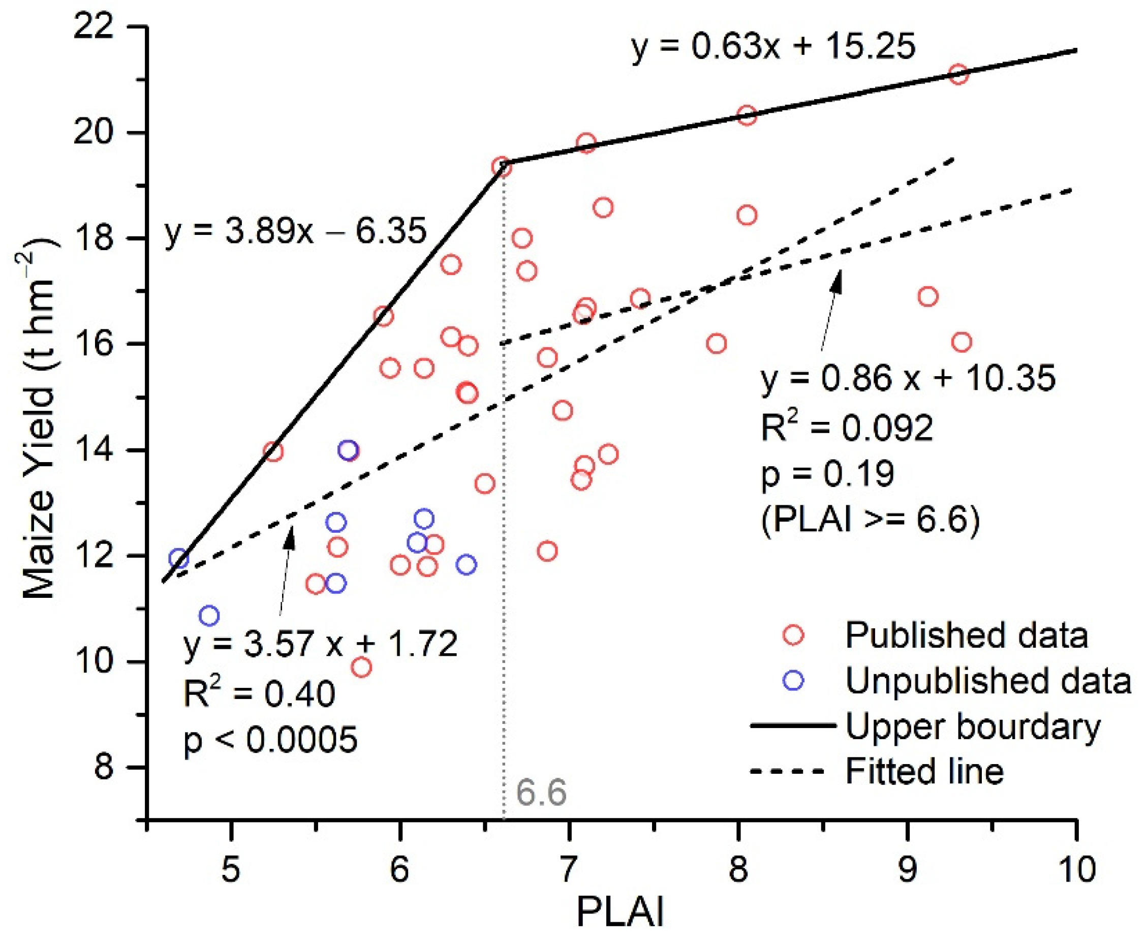
Figure 3.
An example of deriving LAIp from RS-LAI and CREF. LAIp on the right panel (b) was derived by fitting the RS-LAI on the left panel (a) to CREF using the least-square method.
Figure 3.
An example of deriving LAIp from RS-LAI and CREF. LAIp on the right panel (b) was derived by fitting the RS-LAI on the left panel (a) to CREF using the least-square method.
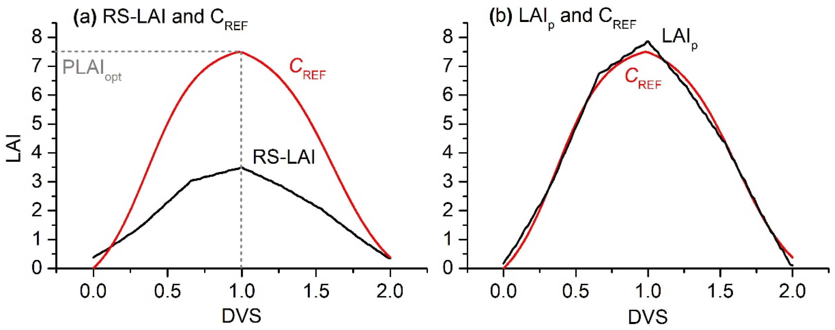
Figure 4.
Maps of modeled Ya of summer maize in 2010 (a), 2011 (b), 2012 (c), 2013 (g), 2014 (h), and 2015 (i); and the pixel-level frequency distribution (FD) of pixel level values in 2010 (d), 2011 (e), 2012 (f), 2013 (j), 2014 (k), and 2015 (l). The scatter plot represents a comparison between modeled yield and reference yield on a prefecture-level, the modeled yield on a prefecture-level is the average of yield values of all pixels within a prefecture-level district, and each scatter plot has 44 samples; the solid line in each scatter plot represents the “1:1 line.” The value ranges in the legend are right-closed and left-open.
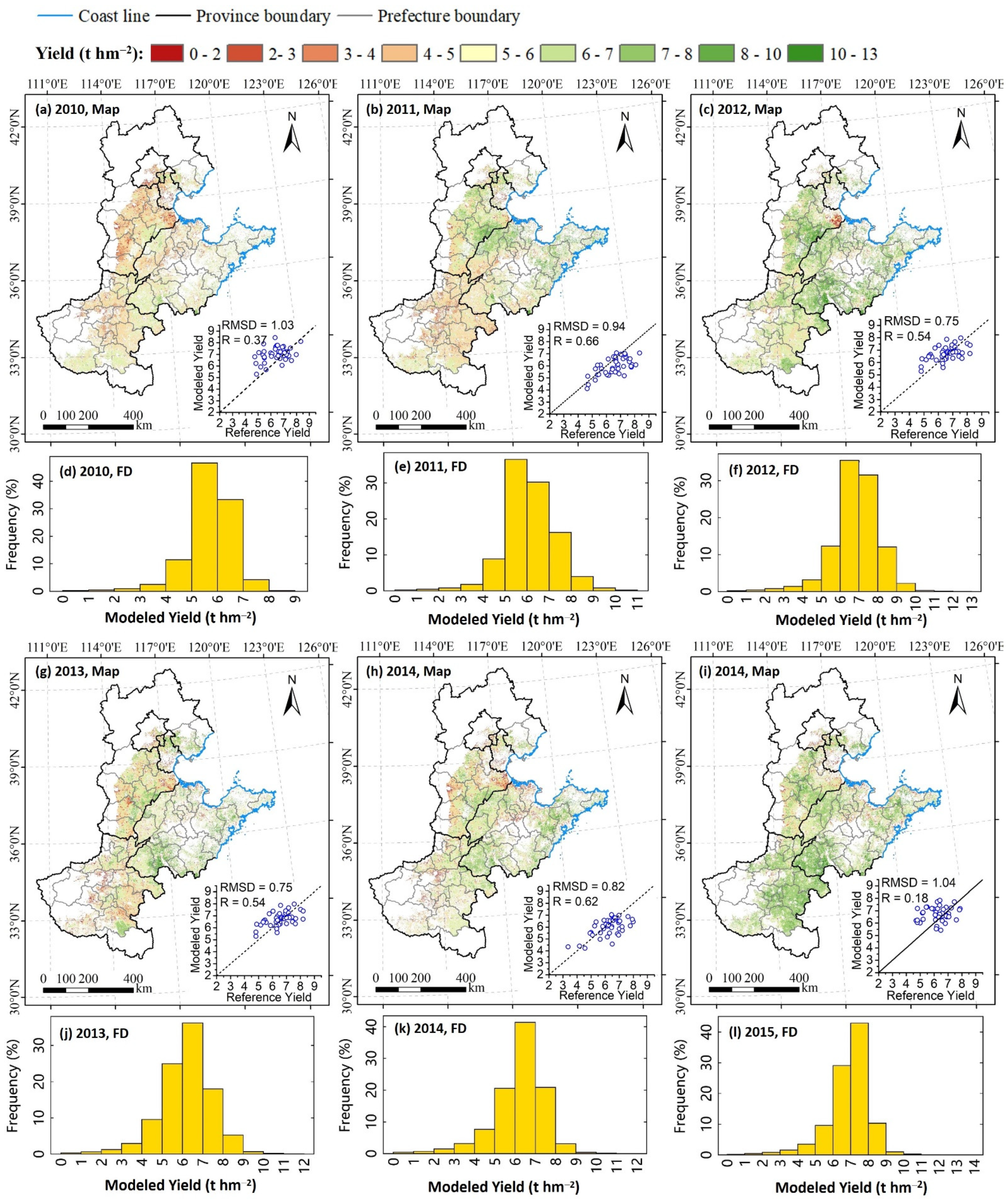
Figure 5.
Modeled maize yields vs. reference values on a prefecture-level for pooled data (a) and mean annual data (b) in the period 2010 to 2015; R, N, and RMSD denote correlation, sample size, and root mean standard deviation, respectively; the error bar represents the standard deviation of multi-year data.
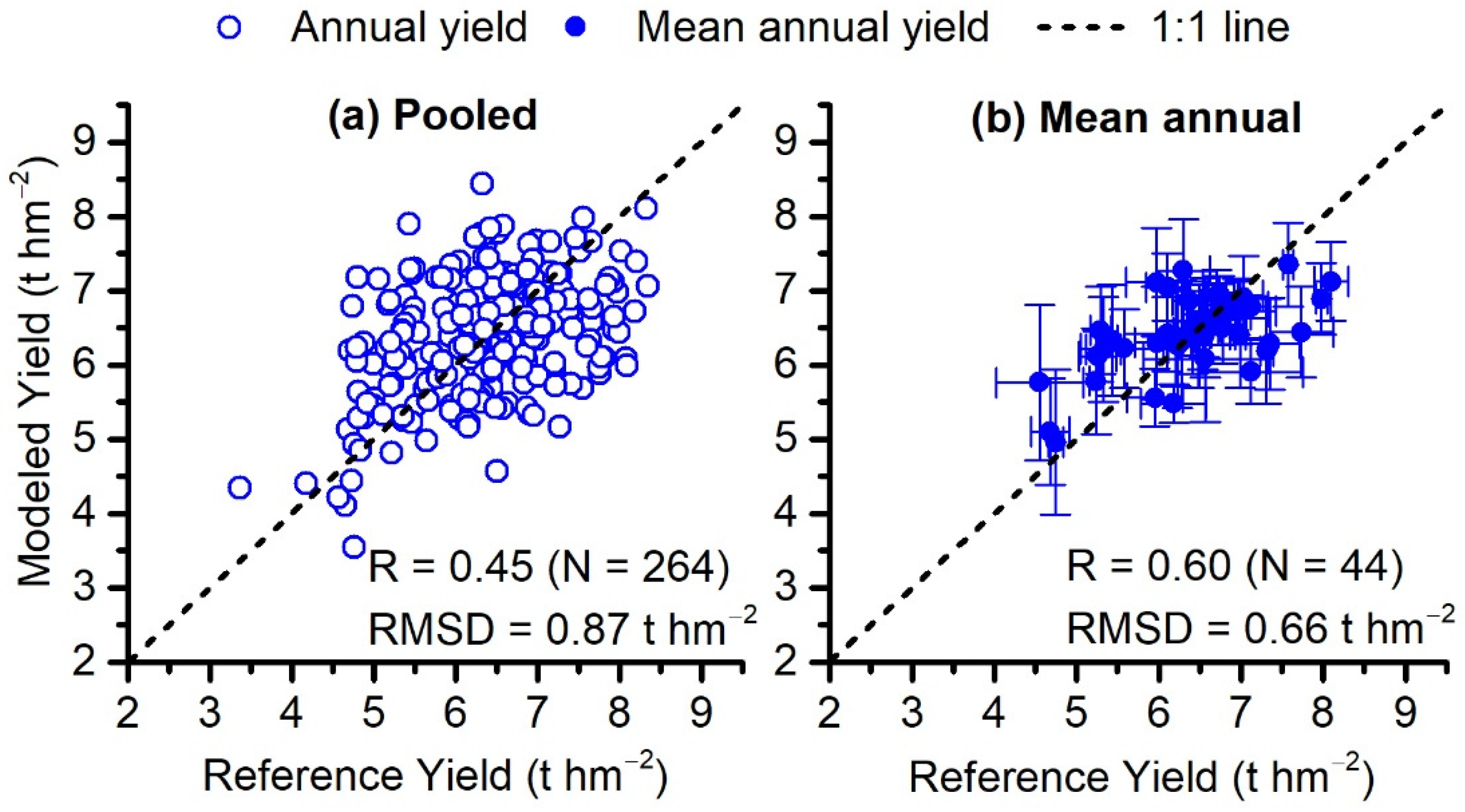
Figure 6.
The map (a) and frequency distribution (b) of mean annual modeled Yp of summer maize over the period 2010 to 2015, and the modeled Yp of 10 agricultural meteorological (AM) sites vs. the simulations of corresponding sites from Wang, Wang, Yin, Feng and Zhang [11] (c). The value ranges in the legend of panel (a) are right-closed and left-open. Yp data from Wang, Wang, Yin, Feng and Zhang [11] represent the average of annual Yp in the period 1982 to 2005 for Linyi, 1982 to 2008 for Zibo and Laiyang, and 1982 to 2009 for the remaining sites.
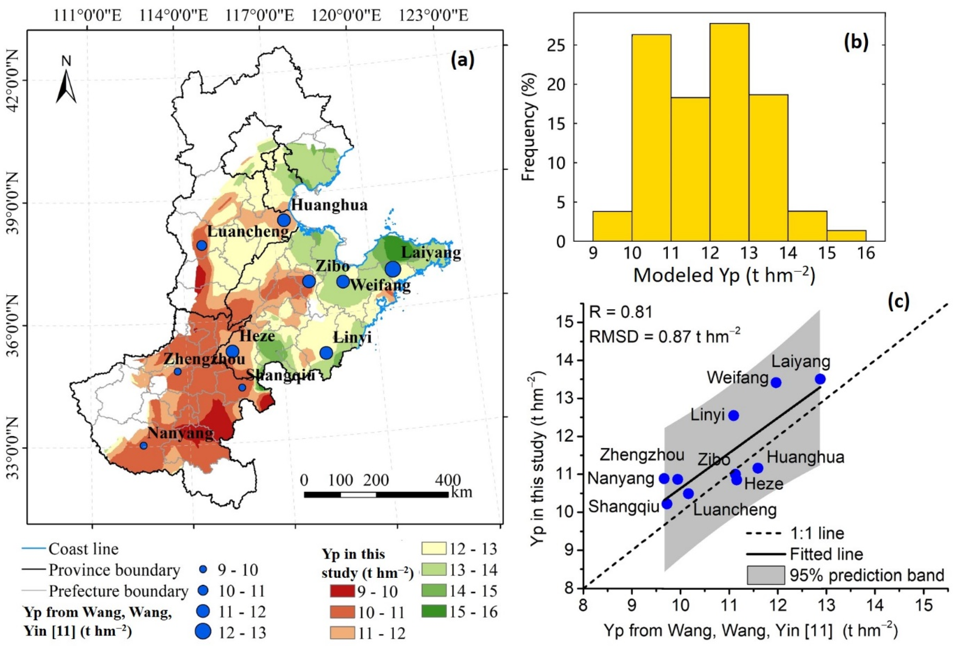
Figure 7.
Annual and the average of the annual regional Yg0, Yp0–Ya, and Ya (a), and proportions of regional Yg0, Yp0–Ya, and Ya in regional Yp (b) in the period 2010 to 2015.
Figure 7.
Annual and the average of the annual regional Yg0, Yp0–Ya, and Ya (a), and proportions of regional Yg0, Yp0–Ya, and Ya in regional Yp (b) in the period 2010 to 2015.
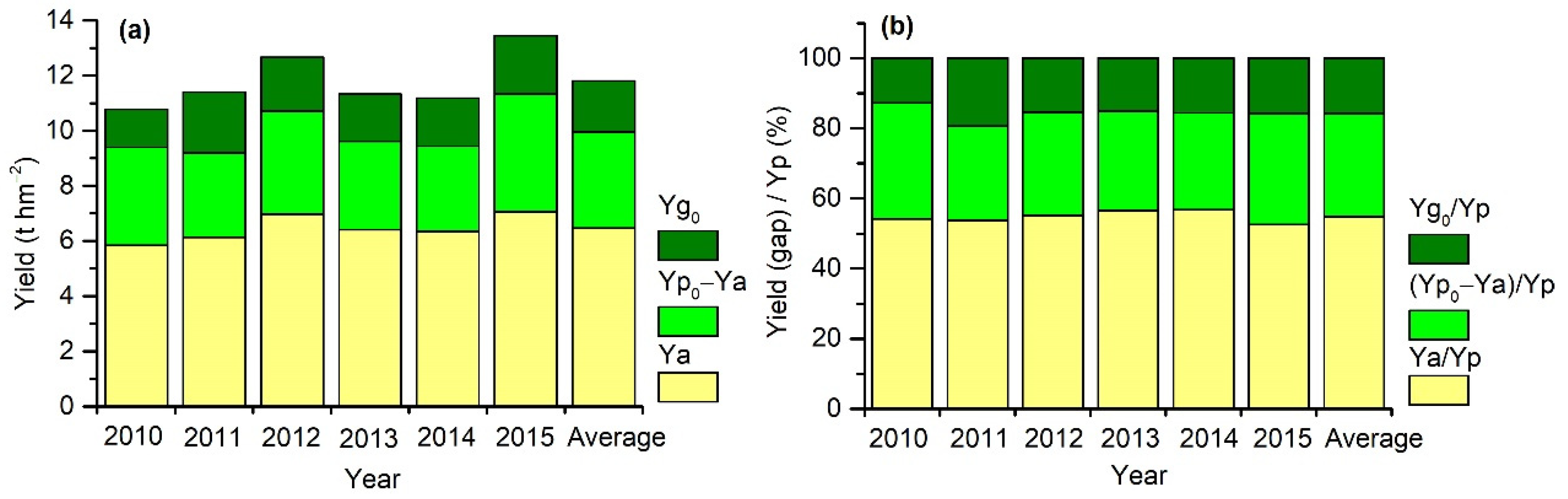
Figure 8.
Maps of simulated mean annual Ya (a), Yg (b), the ratio of Yg to Yp (Yg/Yp) (c), potential yield limited by suboptimum SDT (Yp0) (g), Yg induced by suboptimum SDT(Yg0) (h), and the contribution of suboptimum SDT to Yg (CYg0) (i), with a 5 km resolution in 2010–2015; and the frequency distribution (FD) of pixel-level values of Ya (d), Yg (e), Yg/Yp (f), Yp0 (j), Yg0 (k), and CYg0 (l). The value ranges in the legends are right-closed and left-open. Annual 1 km Ya, Yp0, and Yp were aggregated to 5 km and then averaged in time to derive the mean annual Ya, Yp0, and Yp. Yg and Yg/Yp were derived from the 5 km Ya and Yp, and Yg0 and CYg0 were derived from the 5 km Yp0, Yg, and Yp. Each 5 km grid represents all 1 km cropland pixels inside the grid.


Table 1.
Ya, potential yield limited by suboptimal SDT (Yp0), Yp, Yg, ratio of Yg to Yp (Yg/Yp), ratio of Ya to Yp (Ya/Yp), Yg caused by suboptimal SDT (Yg0), and contribution of suboptimal SDT to Yg (CYg0) in the period 2010 to 2015 for the entire NCP a.
Table 1.
Ya, potential yield limited by suboptimal SDT (Yp0), Yp, Yg, ratio of Yg to Yp (Yg/Yp), ratio of Ya to Yp (Ya/Yp), Yg caused by suboptimal SDT (Yg0), and contribution of suboptimal SDT to Yg (CYg0) in the period 2010 to 2015 for the entire NCP a.
| Year | Ya | Yp | Yg | Yg/Yp | Ya/Yp | Yp0 | Yg0 | CYg0 |
|---|---|---|---|---|---|---|---|---|
| 2010 | 5.8 | 10.8 | 4.9 | 45% | 55% | 9.4 | 1.4 | 29% |
| 2011 | 6.1 | 11.4 | 5.3 | 46% | 54% | 9.2 | 2.2 | 42% |
| 2012 | 7.0 | 12.7 | 5.7 | 45% | 55% | 10.7 | 2.0 | 35% |
| 2013 | 6.4 | 11.3 | 4.9 | 43% | 57% | 9.6 | 1.7 | 35% |
| 2014 | 6.3 | 11.2 | 4.8 | 43% | 57% | 9.4 | 1.8 | 38% |
| 2015 | 7.1 | 13.4 | 6.4 | 48% | 52% | 11.3 | 2.1 | 33% |
| Average | 6.5 | 11.8 | 5.4 | 45% | 55% | 9.9 | 1.9 | 35% |
a Values of Ya, Yp, and Yp0 were computed on the basis of the actual distribution of maize cultivation areas in each year, and Yg/Yp, Ya/Yp, and CYg0 were computed using the regional statistics.
Publisher’s Note: MDPI stays neutral with regard to jurisdictional claims in published maps and institutional affiliations. |
© 2021 by the authors. Licensee MDPI, Basel, Switzerland. This article is an open access article distributed under the terms and conditions of the Creative Commons Attribution (CC BY) license (https://creativecommons.org/licenses/by/4.0/).
Share and Cite
MDPI and ACS Style
Zhang, S.; Bai, Y.; Zhang, J. Remote Sensing-Based Quantification of the Summer Maize Yield Gap Induced by Suboptimum Sowing Dates over North China Plain. Remote Sens. 2021, 13, 3582. https://doi.org/10.3390/rs13183582
AMA Style
Zhang S, Bai Y, Zhang J. Remote Sensing-Based Quantification of the Summer Maize Yield Gap Induced by Suboptimum Sowing Dates over North China Plain. Remote Sensing. 2021; 13(18):3582. https://doi.org/10.3390/rs13183582
Chicago/Turabian StyleZhang, Sha, Yun Bai, and Jiahua Zhang. 2021. "Remote Sensing-Based Quantification of the Summer Maize Yield Gap Induced by Suboptimum Sowing Dates over North China Plain" Remote Sensing 13, no. 18: 3582. https://doi.org/10.3390/rs13183582
Note that from the first issue of 2016, this journal uses article numbers instead of page numbers. See further details here.