
Large Area High-Resolution 3D Mapping of Oxia Planum: The Landing Site for the ExoMars Rosalind Franklin Rover


1
Imaging Group, Mullard Space Science Laboratory, Department of Space and Climate Physics, University College London, Holmbury St Mary, Surrey RH5 6NT, UK
2
Laboratoire de Planétologie et Géodynamique, CNRS, UMR 6112, Université de Nantes, 44300 Nantes, France
3
College of Civil and Transportation Engineering, Shenzhen University, Shenzhen 518060, China
4
Ministry of Natural Resources Key Laboratory for Geo-Environmental Monitoring of Great Bay Area & Guangdong Key Laboratory of Urban Informatics & Shenzhen Key Laboratory of Spatial Smart Sensing and Services, Shenzhen University, Shenzhen 518060, China
*
Author to whom correspondence should be addressed.
Remote Sens. 2021, 13(16), 3270; https://doi.org/10.3390/rs13163270
Submission received: 22 July 2021
/
Revised: 11 August 2021
/
Accepted: 16 August 2021
/
Published: 18 August 2021
(This article belongs to the Special Issue Planetary 3D Mapping, Remote Sensing and Machine Learning)
Abstract
:We demonstrate an end-to-end application of the in-house deep learning-based surface modelling system, called MADNet, to produce three large area 3D mapping products from single images taken from the ESA Mars Express’s High Resolution Stereo Camera (HRSC), the NASA Mars Reconnaissance Orbiter’s Context Camera (CTX), and the High Resolution Imaging Science Experiment (HiRISE) imaging data over the ExoMars 2022 Rosalind Franklin rover’s landing site at Oxia Planum on Mars. MADNet takes a single orbital optical image as input, provides pixelwise height predictions, and uses a separate coarse Digital Terrain Model (DTM) as reference, to produce a DTM product from the given input image. Initially, we demonstrate the resultant 25 m/pixel HRSC DTM mosaic covering an area of 197 km × 182 km, providing fine-scale details to the 50 m/pixel HRSC MC-11 level-5 DTM mosaic. Secondly, we demonstrate the resultant 12 m/pixel CTX MADNet DTM mosaic covering a 114 km × 117 km area, showing much more detail in comparison to photogrammetric DTMs produced using the open source in-house developed CASP-GO system. Finally, we demonstrate the resultant 50 cm/pixel HiRISE MADNet DTM mosaic, produced for the first time, covering a 74.3 km × 86.3 km area of the 3-sigma landing ellipse and partially the ExoMars team’s geological characterisation area. The resultant MADNet HiRISE DTM mosaic shows fine-scale details superior to existing Planetary Data System (PDS) HiRISE DTMs and covers a larger area that is considered difficult for existing photogrammetry and photoclinometry pipelines to achieve, especially given the current limitations of stereo HiRISE coverage. All of the resultant DTM mosaics are co-aligned with each other, and ultimately with the Mars Global Surveyor’s Mars Orbiter Laser Altimeter (MOLA) DTM, providing high spatial and vertical congruence. In this paper, technical details are presented, issues that arose are discussed, along with a visual evaluation and quantitative assessments of the resultant DTM mosaic products.
1. Introduction
Large area, high-resolution, three-Dimensional (3D) mapping of the Martian surface is not only essential for performing key science investigations of the generation and evolution of the planet’s surface, but also critical for supporting existing and future surface robotic missions as well as human exploration. Over the past 20 years, 3D mapping of the Martian surface has only been done for larger areas with lower-resolution data, or for small areas with higher-resolution data.
The large area lower-resolution 3D mapping work usually uses the Mars Express’s High Resolution Stereo Camera (HRSC) data at 12.5–50 m/pixel [1] producing photogrammetric digital terrain models (DTMs) at 50–150 m/pixel [2,3,4,5,6,7], or uses the Mars Reconnaissance Orbiter (MRO) Context Camera (CTX) data at 6 m/pixel [8] producing DTMs at 18–24 m/pixel [9,10,11] where such serendipitous stereo coverage exists.
On the other hand, the small area high-resolution 3D mapping work usually employs the MRO High Resolution Imaging Science Experiment (HiRISE) data at 0.25–0.5 m/pixel [12] producing DTMs at 0.75–2 m/pixel using photogrammetry [13,14,15] or DTMs at 0.25–0.5 m/pixel using photoclinometry [16,17,18,19,20], or uses the ExoMars Trace Gas Orbiter (TGO) Colour and Stereo Surface Imaging System (CaSSIS) data at 4–6 m/pixel [21] producing DTMs at 12–18 m/pixel using photogrammetry [22] or at 4 m/pixel using photoclinometry (at the pixel-level) or at 1 m/pixel using super-resolution restoration assisted photoclinometry [23] (at the sub-pixel level).
The limitations of having to trade-off between “large area” and “high-resolution”, for Mars 3D mapping results from three different aspects. Firstly, lower-resolution data such as HRSC has better stereo coverage as it is inherently a stereo mapping instrument, whereas the main high-resolution data to date (HiRISE) is only capable of targeted stereo. Secondly, the photogrammetry and photoclinometry processes are complex and subject to different errors (or artefacts) at each of their different processing stages, which require specialist expertise to deal with these complexities, in order to produce high-quality DTM products, especially over large areas. Thirdly, the expensive computational cost from the existing photogrammetry and photoclinometry pipelines make it extremely difficult to achieve large area high-resolution coverage.
In this paper, we experiment with a previously developed single-input-image fast DTM surface modelling system, called MADNet (Multi-scale generative Adversarial u-net with Dense convolutional and up-projection blocks) [24], exploring large area high-resolution DTM production using a set of co-registered HRSC-CTX-HiRISE images that are co-aligned with the global reference DTM from the Mars Global Surveyor’s Mars Orbiter Laser Altimeter (MOLA) [25,26,27]. In contrast with traditional photogrammetric methods, where two overlapping images (with a suitable stereo angle, typically ≥8° [10]) are used as inputs to derive the DTM, MADNet requires only a single image as input to derive a DTM, firstly in relative values (normalised), and then uses a referencing coarse DTM (e.g., the globally available MOLA DTM) to produce the final DTM product. It should be noted that the referencing coarse DTM is also required in photogrammetric methods because the initial surface heights, triangulated from the relative image disparities, are generally considered imprecise and are required to be corrected using a reference DTM (typically being the downsampled 463 m/pixel MOLA DTM for Mars). The above differences are illustrated in Figure 1, where we show the simplified flow diagrams of the photogrammetric DTM pipeline and the deep learning-based single-image DTM pipeline (e.g., MADNet [24]).
We focus on the Oxia Planum area [28,29,30,31], where the joint European Space Agency (ESA) and Russian Roscosmos ExoMars mission will land the ESA “Rosalind Franklin” rover and the Roscosmos landing platform “Kazachok” in 2023. Large area high-resolution DTM mosaics, covering the 3-sigma landing ellipses, are produced here at 25 m/pixel for HRSC, 12 m/pixel for CTX, and at 50 cm/pixel for HiRISE. Cascaded 3D co-alignments (HRSC-to-MOLA, CTX-to-HRSC, and HiRISE-to-CTX) have been achieved to guarantee precise global congruence with respect to MOLA. Part of this area has been used for the Jet Propulsion Laboratory webGIS (web based Geographic Information System) called MMGIS (Multi-Mission Geographic Information System) [32] to assist the ExoMars team’s geological characterisation of the area [33].
The layout of this paper is as follows. In Section 2.1, the processing core (MADNet) is reviewed, followed by a comprehensive description of the overall processing chain in Section 2.2. Technical challenges are discussed in Section 2.3, followed by an introduction to the study site. In Section 3.1, Section 3.2 and Section 3.3, we present final results from HRSC, CTX, and HiRISE data, respectively, and these are then followed by Section 3.4 where we present additional assessments for the 50 cm/pixel HiRISE MADNet DTM mosaic. Product access, extensibility of the proposed methods, known issues, limitations, and future work are discussed in Section 4 before conclusions are drawn in Section 5.
2. Materials and Methods
2.1. Overview of MADNet and Training Details
The processing core of this work is the MADNet deep learning based single-image DTM estimation system described in [24]. MADNet is based on the Generative Adversarial Network (GAN) framework [34], and in particular is based on a multi-scale relativistic GAN architecture [35,36], which was previously developed for image super-resolution tasks. MADNet operates by training a generative model for relative height prediction, and in an alternating manner, updating a discriminator model to distinguish the predicted heights from the normalised ground-truth heights.
The MADNet generator network uses a three-scale U-Net [37] based architecture. Each of the three-scale U-Nets (the coarse-scale, intermediate-scale, and fine-scale) consists of a dense convolution block (DCB) [38] based encoder arm and an up-projection block (UPB) [39] based decoder arm. The fine-scale U-Net contains five stacks of convolutional layers, pooling layers, and DCBs to encode the input image into a feature tensor, which is then fed into five stacks of UPBs and convolutional layers with concatenations of the corresponding outputs of each pooling layer to decode the feature vectors into the output height map. The intermediate-scale and coarse-scale U-Nets take two times and four times downsampled input images and use four and three stacks of the convolution-pooling-DCB and UPB-convolution layers to reconstruct the height maps in two times and four times coarser scales, respectively.
Outputs from the three-scale U-Net networks are then merged with adaptive weights to reconstruct the final output height map (relative height). A simplified network architecture of the MADNet generator can be found in Figure 2 for a detailed description (including the discriminator network), please refer to [24].
Training of the MADNet model was achieved in two stages. In the first stage, initial training was performed on each of the three adversarial U-Nets, using 12,600 training pairs of 4 m/pixel (down-sampled) HiRISE images and 8 m/pixel existing HiRISE DTMs. In the second stage, the adaptive weighted multi-scale adversarial U-Nets were trained jointly with weights initialised from the first stage training using 46,500 training pairs of 2 m/pixel HiRISE images and 4 m/pixel HiRISE DTMs. The training pairs contain a collection of different Martian surface features including layers, craters, cones, peaks, dunes, and flat terrains. For detailed hyperparameter setups, please refer to [24].
2.2. Overall Processing Chain
In this work, MADNet is employed alongside 3D co-alignment and DTM mosaicing methods to produce co-aligned DTM mosaics using a set of co-registered HRSC-CTX-HiRISE images over the landing site area. The overall processing chain of the work described here is shown in Figure 3.
The inputs of the proposed large area multi-resolution 3D mapping work are the 463 m/pixel MOLA areoid DTM (available at https://astrogeology.usgs.gov/search/details/Mars/GlobalSurveyor/MOLA/Mars_MGS_MOLA_DEM_mosaic_global_463 m/cub, accessed on 22 July 2021), the 50 m/pixel HRSC MC-11W (Mars Chart-11 West) level 5 DTM mosaic and 12.5 m/pixel ORI mosaic (available at http://hrscteam.dlr.de/HMC30/MC11W/, accessed on 22 July 2021), the 6 m/pixel CTX stereo-view images (accessible through the Arizona State University’s Mars Image Explorer at http://viewer.mars.asu.edu/viewer/ctx, accessed on 22 July 2021), and the 25–50 cm/pixel HiRISE single-view (monocular) images (available through the University of Arizona’s HiRISE site at https://hirise-pds.lpl.arizona.edu/PDS/, accessed on 22 July 2021). The CTX and HiRISE image IDs that cover the landing site area were found through the product coverage shapefile site (https://ode.rsl.wustl.edu/mars/coverage/ODE_Mars_shapefile.html, accessed on 22 July 2021). The final outputs of the mapping work include a 25 m/pixel HRSC DTM mosaic covering about a 197 km × 182 km area of the landing site, a 12 m/pixel CTX DTM mosaic covering about a 114 km × 117 km area of the landing site, and a 50 cm/pixel HiRISE DTM mosaic covering about a 74.3 km × 86.3 km area of the 3-sigma landing ellipses and partially the ExoMars team’s geological characterisation area [33]. It should be noted that all final outputs are 3D co-aligned with the reference MOLA DTM using the B-spline fitting based 3D co-alignment method that was described in [6,23].
The B-spline fitting algorithm described in [6,23] is based on the calculation of the nonrigid closest 3D points of two planar B-spline surfaces computed from the target and reference DTMs. In particular, the nonrigid transformation of each 3D point within the target DTM is calculated by minimising the weighted terms of the distance between the target and reference 3D points, the stiffness values that penalise transformations of the neighbourhood of the target 3D points, and the distance between the 2D tie-points computed from the matching of image features.
The overall processing chain includes 11 steps (labelled in Figure 3) and can be summarised as follows:
- (1)
- B-spline fitting based on 3D co-alignment of the input (cropped) HRSC MC-11W level 5 DTM mosaic with respect to the input MOLA DTM to obtain an intermediate 50 m/pixel MOLA corrected HRSC DTM mosaic.
- (2)
- MADNet DTM production, using the cropped HRSC MC-11W level 5 ORI mosaic as input to produce an intermediate 25 m/pixel HRSC DTM mosaic.
- (3)
- 3D co-alignment of the intermediate 25 m/pixel HRSC DTM mosaic from step (2) and the intermediate 50 m/pixel MOLA-co-aligned HRSC DTM mosaic from step (1), to produce the 25 m/pixel MOLA-co-aligned HRSC DTM mosaic, which is the first of the three final products of this work.
- (4)
- CASP-GO [6,10,40] photogrammetric DTM production of CTX serendipitous “stereo” images to produce 18 m/pixel CTX DTMs, which are co-aligned with the 25 m/pixel MOLA-co-aligned HRSC DTM mosaic from step (3), as well as 6 m/pixel CTX ORIs, which are co-registered with the input 12.5 m/pixel HRSC MC-11W level 5 ORI mosaic.
- (5)
- MADNet DTM production using the intermediate 6 m/pixel HRSC-co-registered CTX ORIs from step (4) to produce intermediate 12 m/pixel CTX DTMs.
- (6)
- 3D co-alignment of the intermediate 12 m/pixel CTX DTMs from step (5) and the 18 m/pixel HRSC-co-aligned CTX DTMs from step (4) to produce 12 m/pixel HRSC-co-aligned CTX DTMs.
- (7)
- DTM mosaicing (using the ASP [40] “dem_mosaic” function) of the 12 m/pixel HRSC-co-aligned CTX DTMs from step (6) to produce a 12 m/pixel HRSC-co-aligned CTX DTM mosaic, which is the second of the three final products of this work.
- (8)
- (9)
- MADNet DTM production using the CTX-co-registered HiRISE images from step (8) to produce intermediate 50 cm/pixel HiRISE DTMs.
- (10)
- 3D co-alignment of the intermediate 50 cm/pixel HiRISE DTMs from step (9) and the 12 m/pixel HRSC-co-aligned CTX DTM mosaic from step (7) to produce CTX-co-aligned 50 cm/pixel HiRISE DTMs.
- (11)
- DTM mosaicing of the 50 cm/pixel CTX-co-aligned HiRISE DTMs from step (10) to produce a 50 cm/pixel CTX-co-aligned HiRISE DTM mosaic, which is the third of the three final products of this work.
It should be noted that the photogrammetric DTMs from HRSC are used as the reference DTM to co-align the HRSC MADNet DTM, because they have a smaller resolution gap in comparison to using the MOLA DTM as the reference. This is also the case for CTX. However, if HRSC and CTX photogrammetric DTMs are not available, the MOLA DTM (for HRSC) and the HRSC MADNet DTM (for CTX) can also be used as the reference datasets. This is demonstrated in the HiRISE case, where photogrammetric processing is far too computationally expensive, and thus not included for HiRISE.
In this work, a total of 12 CTX images (6 serendipitous pairs) and 44 HiRISE images are used (both are manually selected using the list from the aforementioned product coverage shapefile site) to cover the 3-sigma landing ellipses and partially the ExoMars team’s geological characterisation area [33]. The input HiRISE images are manually selected for quality, while keeping sufficient overlaps within neighbouring scenes in order to produce a single uniform quality and gap-free DTM mosaic. The 25 cm/pixel images have a priority over 50 cm/pixel images if both cover the same area. Some HiRISE images that contain severe framelet-stitching artefacts or missing data are excluded. New images are also checked to fill remaining DTM gaps at the end of the process. For full lists of the used CTX and HiRISE image IDs, please refer to Section 3.2 and Section 3.3 It should be noted that there are many more images that exist and are available other than the selected CTX and HiRISE images for this work.
An overview of the area covered, and the input MOLA-HRSC-CTX-HiRISE datasets, are shown in Figure 4. The yellow boxes in Figure 4 represent the coverage of the available HiRISE images (up until NASA’s last released images on 9 June 2021) within the 3-sigma landing ellipses, where the yellow boxes that are shown as hatched fill are HiRISE images with off-nadir counterparts and the plain yellow boxes are HiRISE images without any repeat observations (i.e., only single views are available). As the proposed method only requires single images as inputs, the 3D mapping area for HiRISE can be greatly enlarged to cover other areas without any targeted or serendipitous observations being available.
2.3. Practical Issues and Solutions
Two practical issues occurred while achieving the proposed large area MADNet processing. The first issue refers to the strength of the 3D co-alignment process that converts the MADNet output height map from relative values to absolute values with respect to a low-resolution reference DTM. It should be noted that raw MADNet output height map (in tiles, each 256 × 256 pixels) do not contain any information for the contextual terrain, e.g., large-scale slopes, and such information needs to be recovered from the low-resolution reference DTM using 3D co-alignment. If one insufficiently corrects the raw MADNet outputs, this will result in inaccurate height values or incorrect large-scale topographic variations, and when such errors are large, tiles can no longer be seamlessly mosaiced. On the other hand, over-correcting the raw MADNet outputs will result in small-scale features being smoothed out, and subsequently, local topographic variations becoming extremely low. The strength of the correction is mainly controlled by two weighted terms from the B-spline fitting algorithm [6,23], i.e., the weighted distance between the target and reference 3D points and the weighted stiffness term to penalise transformations of neighbouring 3D points. However, in practice, such weights sometimes need to be manually adjusted depending on different situations, e.g., the surface roughness, topographic characteristics, image quality and effective resolutions. As supervised processing of each single-strip HiRISE DTM is not feasible, we have used a fairly strict set of 3D correction settings, which has a preference towards smoother and less erroneous solutions instead of sharper but more erroneous solutions, and consequently, some minor smoothing issues still exist for the HiRISE results.
Figure 5 shows an example of this issue. We can see the difference between the 50 cm/pixel HiRISE MADNet DTMs with a well-balanced 3D co-alignment (B), and with insufficient 3D co-alignment (A), and inordinate 3D co-alignment (C) with respect to the reference DTM (12 m/pixel CTX MADNet DTM in this case—D). As shown by the individual DTMs and the measured profiles, insufficient 3D co-alignment results in inaccurate DTM heights as well as visible artefacts at the joints between adjacent tiles (there are nine tiles mosaiced together for each of the HiRISE DTMs that are shown in Figure 5), whereas inordinate 3D co-alignment results in seamless mosaicing but with over-smoothed heights. In large area processing, a good set of 3D co-alignment parameters generally works for most of the images (as the images are geographically close and thus have similar topographic properties, e.g., the scales of the slopes are similar), but occasionally, if an image is significantly different to the others, the parameters will need to be adjusted.
The second issue refers to the tiling process of MADNet. Due to the nature of the U-Net based architecture and the limitation of memory of a graphics processing unit, each input image needs to be processed as small overlapping tiles, and the input tile size is fixed at 512 × 512 pixels. For each input image, the number of tiles that need to be processed, depends on the number of overlapping pixels we choose. Generally, a full-strip HiRISE image needs to be divided into 6000 to 12,000 tiles using 100 pixels of overlap, whereas a full-strip CTX image only requires 200 to 300 tiles. Having more overlapping pixels results in a better full-strip mosaic (seamless mosaic) and better tolerance of errors produced by individual tiles. However, when the number of overlapping pixels increases, the number of tiles increases, and consequently the processing time and required storage space also increases. Having insufficient overlapping pixels could result in seamline artefacts around the joints of adjacent tiles. Using 80 to 120 pixels of overlap works for most of the images, but in steep slope areas, this number needs to be increased to achieve seamless mosaicing. Currently, we do not have an automated way of selecting the optimised number of overlapping pixels, so a default number of 100 pixels is used, which results in mostly seamless mosaicing but occasional seamline artefacts.
Figure 6 shows an example of this issue around a sloped area in the HiRISE image (ESP_037703_1980_RED). Although the tiling artefacts are comparably minor (causing a ~10 cm height variation according to the measured profiles) and almost invisible in the DTMs, they are picked up in the hill-shaded images. We can observe that increasing the number of overlapping pixels of adjacent tiles (from 80 pixels to 100 pixels) in MADNet processing helps in reducing the impact of this artefact.
2.4. Study Site
All results shown here are made for the Rosalind Franklin ExoMars 2022 rover’s landing site at Oxia Planum [28,29,30,31]. This site is a 200 km wide clay bearing plain centred on 18.239° N, 24.368° W (see Figure 4) inside the United States Geological Survey (USGS)’s Oxia Palus (MC-11) quadrangle of Mars. The landing site area straddles the dichotomy boundary of Mars, which separates the northern lowlands from the southern highlands. The site slopes towards the north and hosts mineralogical (iron-magnesium rich clay minerals) and geomorphological evidence of liquid water in the ancient past [28,29,30,31], which motivated the choice of this site for this mission whose principal objective is to search for potential biomarkers indicating past life on Mars.
3. Results
In this work, three main sets of 3D products are produced. These are:
- (1)
- The 25 m/pixel HRSC MADNet DTM mosaic (3D co-aligned with the 463 m/pixel MOLA DTM) covering an area of about 197 km × 182 km of the landing site.
- (2)
- The 12 m/pixel CTX MADNet DTM mosaic (3D co-aligned with the 25 m/pixel HRSC MADNet DTM mosaic) and 6 m/pixel CTX ORIs (co-registered with the 12.5 m/pixel HRSC MC-11W level 5 ORI mosaic — “HMC_11W24_nd5”), covering an area of about 114 km × 117 km of the landing site.
- (3)
- The 50 cm/pixel HiRISE MADNet DTM mosaic (3D co-aligned with the 12 m/pixel CTX MADNet DTM mosaic) and 25 cm/pixel HiRISE ORIs (co-registered with the 6 m/pixel CTX ORIs), covering about a 74.3 km × 86.3 km area of the 3-sigma landing ellipses and part of the ExoMars team’s geological characterisation area [33].
In order to maintain a high level of geospatial accuracy of all 3D mapping products produced from this work, precise co-registrations are required between the different resolutions. We achieve cascaded image co-registration and 3D co-alignments with respect to the MOLA DTM and the HRSC MC-11W level 5 ORI mosaic [3], which are considered the most precise and globally consistent topographic geospatial reference of Mars to date, respectively, as our baseline references. In the following three subsections, a qualitative assessment of the MADNet DTM mosaics, alongside the cascaded image co-registration and 3D co-alignment accuracies, is presented for each dataset.
3.1. HRSC Results
Example tiles of the resultant 25 m/pixel HRSC MADNet DTM mosaic are shown in Figure 7. We can observe improved quality, apparent improvement of effective resolution, and reduced noise/artefact in the HRSC MADNet DTM mosaic in comparison to the original HRSC MC-11W level 5 DTM mosaic. From the provided zoom-in views, fine-scale 3D features, e.g., craters and peaks, are better resolved and have more realistic shapes in the HRSC MADNet DTM mosaic compared to the original HRSC MC-11W level 5 DTM mosaic. In particular, the zoom-in view A of Figure 7 shows that the MADNet process is robust against issues in the input image mosaic, i.e., the seamline artefact and obvious resolution changes (caused by mosaicing two HRSC orbits that have different inherent resolutions). The MADNet DTM prediction was not affected by these issues because we cannot observe any artefacts at the location of the seam line.
While the HRSC MC-11W level 5 ORI and DTM mosaics are considered to be precisely co-aligned with the MOLA data, there are still some remaining vertical residuals. In order to achieve a high-standard of MOLA congruence/co-alignment for the HRSC MADNet DTM mosaic and to avoid the propagation of systematic errors from HRSC to the subsequent CTX and HiRISE MADNet DTM mosaics, we perform a further 3D co-alignment process on top of the HRSC MC-11W level 5 DTM mosaic.
The difference maps (at the scale of 500 m/pixel) and scatter plots of the HRSC MC-11W level 5 DTM mosaic (before 3D co-alignment), the HRSC MC-11W level 5 DTM mosaic (after 3D co-alignment), and the HRSC MADNet DTM mosaic, in comparison with the reference MOLA DTM, are shown in Figure 8. We can observe that the HRSC MC-11W level 5 DTM mosaic (after 3D co-alignment) and the HRSC MADNet DTM mosaic shows better overall 3D agreements with the MOLA DTM and reduced systematic errors in comparison to the original HRSC MC-11W level 5 DTM mosaic (before 3D co-alignment). The mean and StdDev (the standard deviation of height differences–provided alongside the difference maps) values have also been reduced slightly.
3.2. CTX Results
The image IDs of the input CTX images are listed in Table 1. The resultant 12 m/pixel CTX MADNet DTM mosaic is shown in Figure 9. We can observe improved quality, apparent resolution, and reduced noise/artefacts in the CTX MADNet DTM mosaic in comparison to the CTX CASP-GO DTMs (produced using photogrammetric methods). From the provided zoom-in views, we can observe more fine scale 3D details of small-scale features and reduction of small-scale noise in the CTX MADNet DTM mosaic. It should be noted that in zoom-in view D of Figure 9, the bumpy “features” shown in the CTX CASP-GO DTM are actually matching artefacts. If we compare the same location within the ORI, such “features” at their scale do not exist. In addition, the two small and connected craters at the western rim of the central crater are not discernible from the CASP-GO DTM. In contrast, the CTX MADNet DTM mosaic shows much better quality for the central crater and the two small craters at the western rim are identifiable. Moreover, zoom-in view D of Figure 9 shows that the MADNet process is robust against issues of small amounts of missing data within the input image, e.g., severe shading effects, where the photogrammetric methods are likely to fail or produce artefacts. It should also be noted that the input CTX ORIs (for MADNet DTM prediction) sometimes contain small-scale artefacts, which could either come from the original CTX data (e.g., patterned stripe lines–see CTX J05_046934_1985_XN_18N025W in Supplementary Materials) or come from the photogrammetric process (e.g., small gaps, local distortions due to image co-registration and transformation), and MADNet has shown moderate robustness to such issues.
In order to achieve a high standard of spatial and vertical accuracy for the CTX MADNet DTM mosaic with respect to MOLA, the CTX CASP-GO ORIs (CTX MADNet input images) are firstly co-registered with the HRSC MC-11W level 5 ORI mosaic, and then the CTX CASP-GO DTMs (CTX MADNet input reference DTMs) are 3D co-aligned with the HRSC MADNet DTM mosaic, which itself is co-aligned with MOLA. Examples showing the image co-registration accuracy between CTX ORIs and the HRSC MC-11W level 5 ORI mosaic or other neighbouring CTX ORIs are presented in Figure 10. We can observe fairly good agreements for both the CTX-to-HRSC and CTX-to-CTX comparisons after the image co-registration process, whereas 50–100 m local displacements are observable before the image co-registration process. The CTX-to-HRSC image co-registration process guarantees a high level of geospatial accuracy of the CTX MADNet DTM processing, as well as being a useful base for subsequent HiRISE processing.
The difference maps (at the scale of 50 m/pixel) and scatter plots of the CTX CASP-GO (photogrammetric) DTM mosaic (before 3D co-alignment), the CTX CASP-GO DTM mosaic (after 3D co-alignment), and the CTX MADNet DTM mosaic, in comparison to the reference HRSC MADNet DTM mosaic (MOLA co-aligned), are shown in Figure 11. We can observe that the CTX CASP-GO DTM mosaic (after 3D co-alignment) and the CTX MADNet DTM mosaic, show much better overall 3D agreements with the HRSC MADNet DTM mosaic (MOLA co-aligned), in comparison to the CTX CASP-GO DTM mosaic (before 3D co-alignment). The mean and StdDev values, provided alongside the difference maps, have also been significantly reduced.
It should be noted that the photogrammetric DTMs from HRSC and CTX are used as the “intermediate” reference DTMs to co-align the HRSC and MADNet DTM in this work, considering the smaller resolution gap (in comparison to using the MOLA DTM as reference) should in theory achieve better 3D co-alignment accuracy. However, lower-resolution reference DTMs (without photogrammetric processing) could also be used as the inputs of the MADNet processing–this is not demonstrated with CTX and HRSC but is demonstrated with HiRISE in this work, where no photogrammetric processing of HiRISE images is involved.
3.3. HiRISE Results
The image IDs of the input HiRISE images are listed in Table 2. The resultant 50 cm/pixel HiRISE MADNet DTM mosaic is shown in Figure 12. In order to demonstrate the quality of the DTM, HiRISE MADNet DTM mosaic (made with 44 single-strip DTMs) are compared against the available HiRISE PDS DTMs (5 in total; image IDs are DTEEC_003195_1985_002694_1985_L01; DTEEC_036925_1985_037558_1985_L01; DTEEC_037070_1985_037136_1985_L01; DTEEC_039299_1985_047501_1985_L01; DTEEC_042134_1985_053962_1985_L01). From the overview, we can observe that there is no systematic bias for the HiRISE MADNet DTM mosaic. From the zoom-in views, we can observe superior DTM quality, more details, higher effective resolution, and reduced noise/artefacts from the HiRISE MADNet DTM mosaic in comparison to the HiRISE PDS DTMs. It should also be noted that some of the input HiRISE images (MADNet input) contain artefacts, such as striping, seamlines, and missing data, however, MADNet shows fairly good robustness to such issues if they appear to be minor (approximately less than 1000 pixels within a 512 × 512 pixels tile).
In order to achieve a high standard of spatial and vertical accuracy for the HiRISE MADNet DTM mosaic with respect to MOLA and HRSC, the input HiRISE images are firstly orthorectified and co-registered with the overlapping CTX CASP-GO ORIs, which themselves are co-registered with the HRSC MC-11W level 5 ORI mosaic. Secondly, the HiRISE MADNet DTM mosaic is spatially corrected with respect to the co-registered HiRISE ORIs. Finally, the HiRISE MADNet DTM mosaic is 3D co-aligned with the CTX MADNet DTM mosaic, which itself is co-aligned with the HRSC MADNet DTM mosaic, which itself is co-aligned with MOLA. Examples showing the image co-registration accuracy between HiRISE ORIs and the CTX ORIs or other neighbouring HiRISE ORIs, are presented in Figure 13. We can observe significant improvements between “before image co-registration” and “after image co-registration”, for both HiRISE-to-CTX and HiRISE-to-HiRISE comparison examples, as local displacements have been reduced from ~100–200 m to subpixel level of the referencing CTX image (≤3 m). The HiRISE-to-CTX image co-registration process guarantees a high level of geospatial accuracy of the resultant HiRISE MADNet DTM mosaic.
The difference maps (at 20 m/pixel) and scatter plots of the HiRISE PDS DTMs and the HiRISE MADNet DTM mosaic, in comparison to the reference CTX MADNet DTM mosaic (HRSC/MOLA co-aligned), are shown in Figure 14. We can observe that the HiRISE MADNet DTM mosaic shows much better overall 3D agreement with the CTX reference in comparison to the HiRISE PDS DTMs. The mean and StdDev values, provided alongside the difference maps, also demonstrate significant improvements. It should be noted that the HiRISE and CTX DTMs are down-sampled and compared at the scale of 20 m/pixel, thus eliminating fine-scale variations, and only show large-scale errors that are greater than 20 m within the difference maps and scatter plots.
3.4. Additional Assessments for the Resultant HiRISE and CTX MADNet DTM Mosaics
In Figure 15, we show the resultant 50 cm/pixel HiRISE MADNet DTM mosaic using hill-shaded images (with a vertical exaggeration factor of 3) using different lighting sources, i.e., 45°, 135°, 225°, and 315° of solar azimuth angles and all at 30° of solar elevation, for four selected areas covering a large crater, small-sized craters, TARs (Transverse Aeolian Ridges), and small peaks. In comparison with the 25 cm/pixel HiRISE ORIs, we observe that the MADNet DTM mosaic has captured fine scale topographic details at a similar effective resolution to the image itself. Hill-shaded images from four different angles demonstrate that there are no obvious errors or artefacts for the selected features. We have included the full-resolution hill-shaded image, a DTM roughness map, and a slope image in the Supplementary Materials.
In Figure 16, we show profile measurements of an example area with a variety of small-sized craters (from 10 m to 30 m diameter). The profiles are measured from the resultant 50 cm/pixel HiRISE MADNet DTM, the 1 m/pixel HiRISE PDS DTM (DTEEC_003195_1985_002694_1985_L01), the 12 m/pixel CTX MADNet DTM, and the 25 m/pixel HRSC MADNet DTM (co-aligned with MOLA). In general, we observe fairly good correlations between all four measured DTMs. The maximum difference between the HiRISE MADNet DTM and the HRSC MADNet DTM is ±10 m (in Profile-1), and the maximum difference between the HiRISE MADNet DTM and the CTX MADNet DTM is ±7 m (in Profile-3). In addition, the HiRISE MADNet DTM shows the best effective resolution compared to the other DTM products and are able to capture many fine-scale features, such as small craters (in all profiles) down to ~5 m in diameter and small peaks (e.g., Profile-5) for sizes down to ~5 m.
On the other hand, we can also observe two types of issues. Firstly, there are some large-scale height differences (of around 3 m to 8 m) between the CTX and HRSC MADNet DTMs. In particular, the behaviour of the higher resolution DTMs (CTX and HiRISE), which display opposing large-scale trends compared with the lower resolution DTM (HRSC), could either be the result of local mis-co-alignment, an inherited photogrammetric error from the HRSC MC-11 DTM, or simply a consequence of the resolution differences between the HRSC and CTX images. In this case, the features from the CTX image are not being properly recorded by HRSC. Although we have achieved fairly good 3D co-alignment accuracy between the CTX and HRSC MADNet DTMs at a much larger scale, as shown in Section 3.2, when zooming into local areas, like Figure 16, height differences still exist. Such height differences (less than 24 m for HRSC-MOLA according to Figure 8 and less than 8 m for CTX-HRSC according to Figure 11) between the baseline DTMs can lower the absolute height accuracy of the HiRISE MADNet DTM even though the HiRISE MADNet DTM has shown “perfect” agreements with the CTX MADNet DTM.
Secondly, we can observe some degradation of features at an intermediate scale (between 120 m and 240 m). For example, the larger crater (in Profile-4 and Profile-5) has more realistic height variations from the HiRISE PDS DTM. Although the HiRISE MADNet DTM has captured much more small-sized craters (with diameter less than 100 m), its large-scale height information is purely dependent on the reference DTM. This is because within each MADNet inference process, the usable input information for MADNet is limited to a tile of 512 × 512 HiRISE pixels (equal to 128 m × 128 m) squared area, which means for craters that are larger than 128 m × 128 m (equal to ~20 × 20 CTX pixels), their reconstruction quality is actually based on the MADNet processing of the CTX images.
From Figure 16, we can observe that the smallest craters we can retrieve through MADNet applied to HiRISE are about 2 m in diameter, and for a good quality retrieval, the diameter is probably about 10 m. This approximates to an area of 40 × 40 pixels of the HiRISE image. As the same rule also applies to CTX images, we should therefore have good reconstructions of features (e.g., craters) that are larger than 240 m × 240 m from CTX (i.e., 40 × 40 CTX pixels). Counting the HiRISE tile size being 128 m × 128 m, HiRISE MADNet DTM theoretically has a weakness for detecting features at this intermediate scale, i.e., between 128 m × 128 m and 240 m × 240 m.
This is generally not an issue for MADNet processing of CTX and CaSSIS images as the resolution gap between the CTX/CaSSIS images and the reference HRSC DTMs is much smaller compared to the resolution gap between the HiRISE images and the reference CTX DTMs. However, this could be an issue for MADNet processing of HRSC images if HRSC photogrammetric DTMs are not available, and where MOLA has to be used. We are exploring potential solutions to this issue (see discussions in Section 4.4).
4. Discussion
4.1. Product Access
The resultant HRSC, CTX, and HiRISE DTM mosaics and ORIs for the Oxia Planum landing site will be made available through the ESA Guest Storage Facility (GSF; see https://www.cosmos.esa.int/web/psa/ucl-mssl_meta-gsf, accessed on 22 July 2021). Before this becomes available, please contact the authors for access to the products.
4.2. Extensibility with Other Satasets or Area
The original MADNet work [24] was demonstrated using the 4 m/pixel CaSSIS images. With only minor changes and parameter tuning, the same DTM production system has been applied to the 12.5 m/pixel HRSC, 6 m/pixel CTX, and 25–50 cm/pixel HiRISE images for a much larger area in this work. Typical barriers in planetary 3D mapping, such as find suitable stereo pairs, potential complication of surface albedos, and expensive computational costs, are avoided using the demonstrated method. The extensibility is thus considered high and applications to other Mars datasets, e.g., the 50 cm/pixel Tianwen-1 High Resolution Imaging Camera (HiRIC) images [43], lunar datasets (retraining can be achieved using the Lunar Reconnaissance Orbiter Camera Narrow Angle Camera images [44] and existing PDS DTM products), and/or other planetary datasets, could be straightforwardly explored in the future.
4.3. Known Artefact
The resultant 50 cm/pixel HiRISE MADNet DTM mosaic has some known artefacts. These include the aforementioned tiling artefacts and smoothing issues that were discussed in Section 2.3 and Section 3.4, respectively, DTM gaps due to insufficient overlap of HiRISE images, and linear artefacts due to missing data within the HiRISE image (only found in strips). Figure 17 provides an example for each of the four known artefacts within the hill-shaded images and show how much they would affect the DTMs. The affected areas are considered minor (less than 0.2% of the total number of pixels) within the mosaic. It should also be noted that the HRSC and CTX MADNet DTM mosaics do not have any of these artefacts.
4.4. Limitations and Future Work
Currently, the proposed MADNet based DTM processing chain has two main limitations. The first limitation is the introduction of tiling artefacts to the final product. Although we do not observe sharp transitions between each MADNet tile (a typical height difference across the tile boundaries is ~10 cm), sometimes two adjacent tiles may have different inference performance that results in different levels of detail, and subsequently results in different appearance in a full-strip DTM mosaic (see issues raised in Section 2.3). We are exploring potential solutions to this issue, for example, adapting the MADNet architecture to focus on fine-scale reconstructions only, using “flattened” training DTMs (large-scale slopes being removed), and leaving out the coarse-scale reconstruction with the low-resolution reference DTM.
The second limitation is regarding the reference data. While introducing photogrammetric DTMs as reference data gives better 3D accuracy to the resultant MADNet DTMs, in comparison to using the very low-resolution MOLA DTM as reference (see issues discussed in Section 3.4), we are aware that there are some photogrammetric DTM artefacts that may get propagated into the MADNet DTMs through the 3D co-alignment process.
In this work, we use a multi-stage strategy to gradually produce a 50 cm/pixel HiRISE DTM when propagating coarse-to-fine information from 463 m/pixel MOLA DTM to 50 m/pixel HRSC DTM, to 25 m/pixel HRSC MADNet DTM, to 18 m/pixel CTX DTM, to 12 m/pixel CTX MADNet DTM, and then to 50 cm/pixel HiRISE MADNet DTM. Each step has inevitably inherited photogrammetric DTM artefacts, but these get reduced with the MADNet processing. However, such inherited photogrammetric DTM artefacts still cannot be fully eliminated despite our best efforts to date.
In the future, we will explore potential solutions like the use of a pyramidal coarse-to-fine approach on the full-sized input image itself on top of the existing pyramidal scheme within individual tiles. This will allow incremental corrections of large-scale inherited photogrammetric errors and also address the issue of the resolution gaps between target images and reference DTMs as mentioned in Section 3.4.
Finally, finding automated ways to solve the issues described in Section 2.3 will also be part of future work. Combining MADNet with image super-resolution restoration [36] or shape-from-shading techniques [23] will also be explored in the future.
5. Conclusions
In this paper, we demonstrate an end-to-end application using the MADNet DTM surface modelling system [24] to create large area, multi- and high-resolution 3D mapping products from HRSC, CTX, and HiRISE single images that are co-aligned with each other and MOLA baseline DTM over the ExoMars 2022 Rosalind Franklin rover’s landing site, at Oxia Planum. Technical issues are discussed and assessments are provided. We believe the demonstrated DTM mosaic products have state-of-the-art DTM quality and geospatial accuracy with respect to MOLA. Moreover, the resultant HiRISE MADNet DTM mosaic covers the whole 3-sigma landing ellipses for the first time at 50 cm/pixel resolution with uniform quality and consistency. All resultant DTM products will be made publicly available alongside this paper.
Supplementary Materials
The following are available online. DTM and ORI results, derived products, and figures at full resolution are available online at https://liveuclac-my.sharepoint.com/:f:/g/personal/ucasyta_ucl_ac_uk/EnrEek4jUppMkh5c7mBPAEwBwLUsO_MgoJWyLpQaLmN1Jw?e=jBcwEo, accessed on 22 July 2021.
Author Contributions
Conceptualization, Y.T., J.-P.M. and S.J.C.; methodology, Y.T.; software, Y.T.; validation, Y.T., J.-P.M. and S.J.C.; formal analysis, Y.T.; investigation, Y.T. and J.-P.M.; resources, Y.T., J.-P.M., S.J.C. and S.X.; data curation, Y.T., J.-P.M. and S.X.; writing—original draft preparation, Y.T.; writing—review and editing, Y.T., J.-P.M. and S.X.; visualization, Y.T. and S.X.; supervision, Y.T. and J.-P.M.; project administration, Y.T. and J.-P.M.; funding acquisition, Y.T., J.-P.M. and S.J.C. All authors have read and agreed to the published version of the manuscript.
Funding
The research leading to these results is receiving funding from the UKSA Aurora programme (2018–2021) under grant no. ST/S001891/1, as well as partial funding from the STFC MSSL Consolidated Grant ST/K000977/1. S.C. is grateful to the French Space Agency CNES for supporting her HiRISE related work. S.X. has received funding from the Shenzhen Scientific Research and Development Funding Programme (grant No. JCYJ20190808120005713) and China Postdoctoral Science Foundation (grant No. 2019M663073).
Institutional Review Board Statement
Not applicable.
Informed Consent Statement
Not applicable.
Data Availability Statement
The output results will all be publicly available and open access. See https://www.cosmos.esa.int/web/psa/ucl-mssl_meta-gsf, accessed on 22 July 2021.
Acknowledgments
The research leading to these results is receiving funding from the UKSA Aurora programme (2018–2021) under grant ST/S001891/1, as well as partial funding from the STFC MSSL Consolidated Grant ST/K000977/1. S.C. is grateful to the French Space Agency CNES for supporting her HiRISE related work. Support from SGF (Budapest), the University of Arizona (Lunar and Planetary Lab.), and NASA are also gratefully acknowledged. Operations support from the UK Space Agency under grant ST/R003025/1 is also acknowledged. S.X. has received funding from the Shenzhen Scientific Research and Development Funding Programme (grant No. JCYJ20190808120005713) and China Postdoctoral Science Foundation (grant No. 2019M663073). The authors would like to thank the HRSC, CTX, and HiRISE teams for making these images and derived products publicly available.
Conflicts of Interest
The authors declare no conflict of interest.
References
- Neukum, G.; Jaumann, R. HRSC: The high resolution stereo camera of Mars Express. Sci. Payload 2004, 1240, 17–35. [Google Scholar]
- Gwinner, K.; Scholten, F.; Preusker, F.; Elgner, S.; Roatsch, T.; Spiegel, M.; Schmidt, R.; Oberst, J.; Jaumann, R.; Heipke, C. Topography of Mars from global mapping by HRSC high-resolution digital terrain models and orthoimages: Characteristics and performance. Earth Planet. Sci. Lett. 2010, 294, 506–519. [Google Scholar] [CrossRef]
- Gwinner, K.; Jaumann, R.; Hauber, E.; Hoffmann, H.; Heipke, C.; Oberst, J.; Neukum, G.; Ansan, V.; Bostelmann, J.; Dumke, A.; et al. The High Resolution Stereo Camera (HRSC) of Mars Express and its approach to science analysis and mapping for Mars and its satellites. Planet. Space Sci. 2016, 126, 93–138. [Google Scholar] [CrossRef]
- Gwinner, K.; Scholten, F.; Spiegel, M.; Schmidt, R.; Giese, B.; Oberst, J.; Heipke, C.; Jaumann, R.; Neukum, G. Derivation and validation of high-resolution digital terrain models from Mars Express HRSC data. Photogramm. Eng. Remote. Sens. 2009, 75, 1127–1142. [Google Scholar] [CrossRef] [Green Version]
- O’Hara, R.; Barnes, D. A new shape from shading technique with application to Mars Express HRSC images. ISPRS J. Photogramm. Remote. Sens. 2012, 67, 27–34. [Google Scholar] [CrossRef]
- Tao, Y.; Michael, G.; Muller, J.P.; Conway, S.J.; Putri, A.R. Seamless 3 D Image Mapping and Mosaicing of Valles Marineris on Mars Using Orbital HRSC Stereo and Panchromatic Images. Remote. Sens. 2021, 13, 1385. [Google Scholar] [CrossRef]
- Putri, A.R.D.; Sidiropoulos, P.; Muller, J.P.; Walter, S.H.; Michael, G.G. A new south polar digital terrain model of Mars from the High-Resolution Stereo Camera (HRSC) onboard the ESA Mars Express. Planet. Space Sci. 2019, 174, 43–55. [Google Scholar] [CrossRef]
- Malin, M.C.; Bell, J.F.; Cantor, B.A.; Caplinger, M.A.; Calvin, W.M.; Clancy, R.T.; Edgett, K.S.; Edwards, L.; Haberle, R.M.; James, P.B.; et al. Context camera investigation on board the Mars Reconnaissance Orbiter. J. Geophys. Res. Space Phys. 2007, 112, 112. [Google Scholar] [CrossRef] [Green Version]
- Wang, Y.; Wu, B. Investigation of boresight offsets and co-registration of HiRISE and CTX imagery for precision Mars topographic mapping. Planet. Space Sci. 2017, 139, 18–30. [Google Scholar] [CrossRef]
- Tao, Y.; Muller, J.P.; Sidiropoulos, P.; Xiong, S.T.; Putri, A.R.D.; Walter, S.H.G.; Veitch-Michaelis, J.; Yershov, V. Massive stereo-based DTM production for Mars on cloud computers. Planet. Space Sci. 2018, 154, 30–58. [Google Scholar] [CrossRef]
- Chen, Z.; Wu, B.; Liu, W.C. Mars3DNet: CNN-Based High-Resolution 3D Reconstruction of the Martian Surface from Single Images. Remote. Sens. 2021, 13, 839. [Google Scholar] [CrossRef]
- McEwen, A.S.; Eliason, E.M.; Bergstrom, J.W.; Bridges, N.T.; Hansen, C.J.; Delamere, W.A.; Grant, J.A.; Gulick, V.C.; Herkenhoff, K.E.; Keszthelyi, L.; et al. Mars reconnaissance orbiter’s high resolution imaging science experiment (HiRISE). J. Geophys. Res. Space Phys. 2007, 112, E05S02. [Google Scholar] [CrossRef] [Green Version]
- Kirk, R.L.; Howington-Kraus, E.; Rosiek, M.R.; Cook, D.; Anderson, J.; Becker, K.; Archinal, B.A.; Keszthelyi, L.; King, R.; McEwen, A.S.; et al. Ultrahigh resolution topographic mapping of Mars with HiRISE stereo images: Methods and first results. In Proceedings of the Seventh International Conference on Mars, Moscow, Russia, 9 July 2007; p. 3381. [Google Scholar]
- Kim, J.R.; Muller, J.P. Very high resolution stereo DTM extraction and its application to surface roughness estimation over Martian surface. Int. Arch. Photogramm. Remote. Sens. Spat. Inf. Sci. 2008, 37, 993–998. [Google Scholar]
- Kim, J.R.; Muller, J.P. Multi-resolution topographic data extraction from Martian stereo imagery. Planet. Space Sci. 2009, 57, 2095–2112. [Google Scholar] [CrossRef]
- Beyer, R.A.; McEwen, A.S.; Kirk, R.L. Meter-scale slopes of candidate MER landing sites from point photoclinometry. J. Geophys. Res. Planets 2003, 108, E12. [Google Scholar] [CrossRef]
- Douté, S.; Jiang, C. Small-Scale Topographical Characterization of the Martian Surface With In-Orbit Imagery. IEEE Trans. Geosci. Remote. Sens. 2019, 58, 447–460. [Google Scholar] [CrossRef]
- Jiang, C.; Douté, S.; Luo, B.; Zhang, L. Fusion of photogrammetric and photoclinometric information for high-resolution DEMs from Mars in-orbit imagery. ISPRS J. Photogramm. Remote. Sens. 2017, 130, 418–430. [Google Scholar] [CrossRef]
- Hess, M.; Wohlfarth, K.; Grumpe, A.; Wöhler, C.; Ruesch, O.; Wu, B. Atmospherically compensated shape from shading on the martian surface: Towards the perfect digital terrain model of mars. Int. Arch. Photogramm. Remote. Sens. Spat. Inf. Sci. 2019, XLII-2/W13, 1405–1411. [Google Scholar] [CrossRef] [Green Version]
- Hess, M. High Resolution Digital Terrain Model for the Landing Site of the Rosalind Franklin (ExoMars) Rover. Adv. Space Res. 2019, 53, 1735–1767. [Google Scholar]
- Thomas, N.; Cremonese, G.; Ziethe, R.; Gerber, M.; Brändli, M.; Bruno, G.; Erismann, M.; Gambicorti, L.; Gerber, T.; Ghose, K.; et al. The colour and stereo surface imaging system (CaSSIS) for the ExoMars trace gas orbiter. Space Sci. Rev. 2017, 212, 1897–1944. [Google Scholar] [CrossRef] [Green Version]
- Simioni, E.; Re, C.; Mudric, T.; Cremonese, G.; Tulyakov, S.; Petrella, A.; Pommerol, A.; Thomas, N. 3DPD: A photogrammetric pipeline for a PUSH frame stereo cameras. Planet. Space Sci. 2021, 198, 105165. [Google Scholar] [CrossRef]
- Tao, Y.; Douté, S.; Muller, J.P.; Conway, S.J.; Thomas, N.; Cremonese, G. Ultra-High-Resolution 1 m/pixel CaSSIS DTM Using Super-Resolution Restoration and Shape-from-Shading: Demonstration over Oxia Planum on Mars. Remote. Sens. 2021, 13, 2185. [Google Scholar] [CrossRef]
- Tao, Y.; Xiong, S.; Conway, S.J.; Muller, J.-P.; Guimpier, A.; Fawdon, P.; Thomas, N.; Cremonese, G. Rapid Single Image-Based DTM Estimation from ExoMars TGO CaSSIS Images Using Generative Adversarial U-Nets. Remote. Sens. 2021, 13, 2877. [Google Scholar] [CrossRef]
- Smith, D.E.; Zuber, M.T.; Frey, H.V.; Garvin, J.B.; Head, J.W.; Muhleman, D.O.; Pettengill, G.H.; Phillips, R.J.; Solomon, S.C.; Zwally, H.J.; et al. Mars Orbiter Laser Altimeter—Experiment summary after the first year of global mapping of Mars. J. Geophys. Res. 2001, 106, 23689–23722. [Google Scholar] [CrossRef]
- Neumann, G.A.; Rowlands, D.D.; Lemoine, F.G.; Smith, D.E.; Zuber, M.T. Crossover analysis of Mars Orbiter Laser Altimeter data. J. Geophys. Res. 2001, 106, 23753–23768. [Google Scholar] [CrossRef] [Green Version]
- Albee, A.L.; Arvidson, R.E.; Palluconi, F.; Thorpe, T. Overview of the Mars Global Surveyor mission. J. Geophys. Res. 2001, 106, 23291–23316. [Google Scholar] [CrossRef] [Green Version]
- Quantin-Nataf, C.; Carter, J.; Mandon, L.; Thollot, P.; Balme, M.; Volat, M.; Pan, L.; Loizeau, D.; Millot, C.; Breton, S.; et al. Oxia Planum: The Landing Site for the ExoMars “Rosalind Franklin” Rover Mission: Geological Context and Prelanding Interpretation. Astrobiology 2021, 21, 345–366. [Google Scholar] [CrossRef] [PubMed]
- Favaro, E.A.; Balme, M.R.; Davis, J.M.; Grindrod, P.M.; Fawdon, P.; Barrett, A.M.; Lewis, S.R. The Aeolian Environment of the Landing Site for the ExoMars Rosalind Franklin Rover in Oxia Planum, Mars. J. Geophys. Res. Planets 2021, 126, 2020JE006723. [Google Scholar] [CrossRef]
- Ivanov, M.A.; Slyuta, E.N.; Grishakina, E.A.; Dmitrovskii, A.A. Geomorphological analysis of ExoMars candidate landing site Oxia Planum. Sol. Syst. Res. 2020, 54, 1–14. [Google Scholar] [CrossRef]
- Mandon, L.; Parkes Bowen, A.; Quantin-Nataf, C.; Bridges, J.C.; Carter, J.; Pan, L.; Beck, P.; Dehouck, E.; Volat, M.; Thomas, N.; et al. Morphological and Spectral Diversity of the Clay-Bearing Unit at the ExoMars Landing Site Oxia Planum. Astrobiology 2021, 21, 464–480. [Google Scholar] [CrossRef]
- Calef, F.J., III; Gengl, H.E.; Soliman, T.; Abercrombie, S.P.; Powell, M.W. MMGIS: A Multi-Mission Geographic Information System for in situ Mars Operations. In Proceedings of the Liquid Propulsion Systems Centre 2017, The Woodlands, TX, USA, 20–24 March 2017; Volume XLVIII, p. 2541. [Google Scholar]
- Sefton-Nash, E.; Fawdon, P.; Orgel, C.; Balme, M.; Quantin-Nataf, C.; Volat, M.; Hauber, E.; Adeli, S.; Davis, J.; Grindrod, P.; et al. Exomars RSOWG. Team Mapping of Oxia Planum for The Exomars 2022 Rover-Surface Platform Mission. In Proceedings of the Liquid Propulsion Systems Centre 2021, 19–30 April 2021; Volume 52, p. 1947. [Google Scholar]
- Goodfellow, I.J.; Pouget-Abadie, J.; Mirza, M.; Xu, B.; Warde-Farley, D.; Ozair, S.; Courville, A.; Bengio, Y. Generative adversarial networks. arXiv 2014, arXiv:1406.2661. [Google Scholar]
- Jolicoeur-Martineau, A. The relativistic discriminator: A key element missing from standard GAN. arXiv 2018, arXiv:1807.00734. [Google Scholar]
- Tao, Y.; Conway, S.J.; Muller, J.-P.; Putri, A.R.D.; Thomas, N.; Cremonese, G. Single Image Super-Resolution Restoration of TGO CaSSIS Colour Images: Demonstration with Perseverance Rover Landing Site and Mars Science Targets. Remote. Sens. 2021, 13, 1777. [Google Scholar] [CrossRef]
- Ronneberger, O.; Fischer, P.; Brox, T. U-net: Convolutional networks for biomedical image segmentation. In Proceedings of the International Conference on Medical Image Computing and Computer-Assisted Intervention, Munich, Germany, 18 May 2015; pp. 234–241. [Google Scholar]
- Huang, G.; Liu, Z.; Van Der Maaten, L.; Weinberger, K.Q. Densely connected convolutional networks. In Proceedings of the IEEE Conference on Computer Vision and Pattern Recognition, Donostia, Spain, 5–8 June 2017; pp. 4700–4708. [Google Scholar]
- Laina, I.; Rupprecht, C.; Belagiannis, V.; Tombari, F.; Navab, N. Deeper depth prediction with fully convolutional residual networks. In Proceedings of the 2016 IEEE Fourth international Conference on 3D Vision (3DV), Stanford, CA, USA, 25 October 2016; pp. 239–248. [Google Scholar]
- Beyer, R.; Alexandrov, O.; McMichael, S. The Ames Stereo Pipeline: NASA’s Opensource Software for Deriving and Processing Terrain Data. Earth Space Sci. 2018, 5, 537–548. [Google Scholar] [CrossRef]
- Tao, Y.; Muller, J.-P.; Poole, W.D. Automated localisation of Mars rovers using co-registered HiRISE-CTX-HRSC orthorectified images and DTMs. Icarus 2016, 280, 139–157. [Google Scholar] [CrossRef] [Green Version]
- Cai, G.R.; Jodoin, P.M.; Li, S.Z.; Wu, Y.D.; Su, S.Z.; Huang, Z.K. Perspective-SIFT: An efficient tool for low-altitude remote sensing image registration. Signal. Process. 2013, 93, 3088–3110. [Google Scholar] [CrossRef]
- Meng, Q.; Wang, D.; Wang, X.; Li, W.; Yang, X.; Yan, D.; Li, Y.; Cao, Z.; Ji, Q.; Sun, T.; et al. High Resolution Imaging Camera (HiRIC) on China’s First Mars Exploration Tianwen-1 Mission. Space Sci. Rev. 2021, 217, 1–29. [Google Scholar] [CrossRef]
- Robinson, M.S.; Brylow, S.M.; Tschimmel, M.; Humm, D.; Lawrence, S.J.; Thomas, P.C.; Denevi, B.W.; Bowman-Cisneros, E.; Zerr, J.; Ravine, M.A.; et al. Lunar reconnaissance orbiter camera (LROC) instrument overview. Space Sci. Rev. 2010, 150, 81–124. [Google Scholar] [CrossRef]
Figure 1.
Illustration of the major differences between the photogrammetric DTM pipeline and the deep learning-based single-image DTM pipeline (e.g., MADNet) discussed here.
Figure 1.
Illustration of the major differences between the photogrammetric DTM pipeline and the deep learning-based single-image DTM pipeline (e.g., MADNet) discussed here.

Figure 2.
Overview of the MADNet generator network architecture. The input image has a size of 512 × 512 pixels and the final output height map has a size of 256 × 256 pixels in a relative value range of (0, 1).
Figure 2.
Overview of the MADNet generator network architecture. The input image has a size of 512 × 512 pixels and the final output height map has a size of 256 × 256 pixels in a relative value range of (0, 1).

Figure 3.
Overall processing chain of the large area multi-resolution (HRSC-CTX-HiRISE) 3D mapping work. Inputs are shown with the light orange boxes, intermediate products with the light blue boxes, and final outputs are shown with the light green boxes.
Figure 3.
Overall processing chain of the large area multi-resolution (HRSC-CTX-HiRISE) 3D mapping work. Inputs are shown with the light orange boxes, intermediate products with the light blue boxes, and final outputs are shown with the light green boxes.
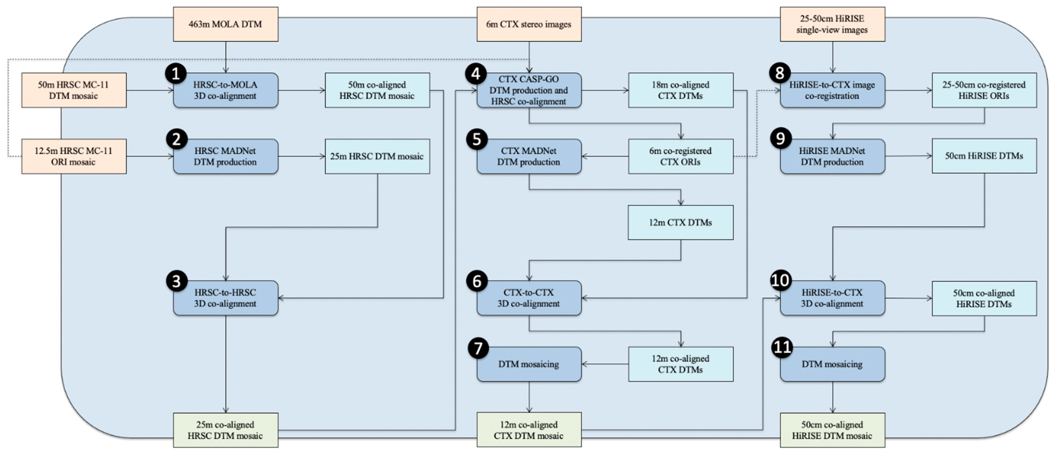
Figure 4.
An overview of the proposed 3D mapping area at Oxia Planum (centred at 18.239°N, 24.368°W), showing the ESA Rosalind Franklin rover 2022 1-sigma (red) and 3-sigma (green) landing ellipse areas and the ExoMars team’s geological characterisation area (blue). Shown in the background are the co-registered input datasets of MOLA DTM (colourised and hill-shaded), cropped HRSC MC-11W level 5 ORI greyscale mosaic, CTX ORI mosaic, and HiRISE image footprints (in yellow; with hatched outlines referring to those available with off-nadir stereo; the footprints are relevant to the NASA release data of 9 June 2021).
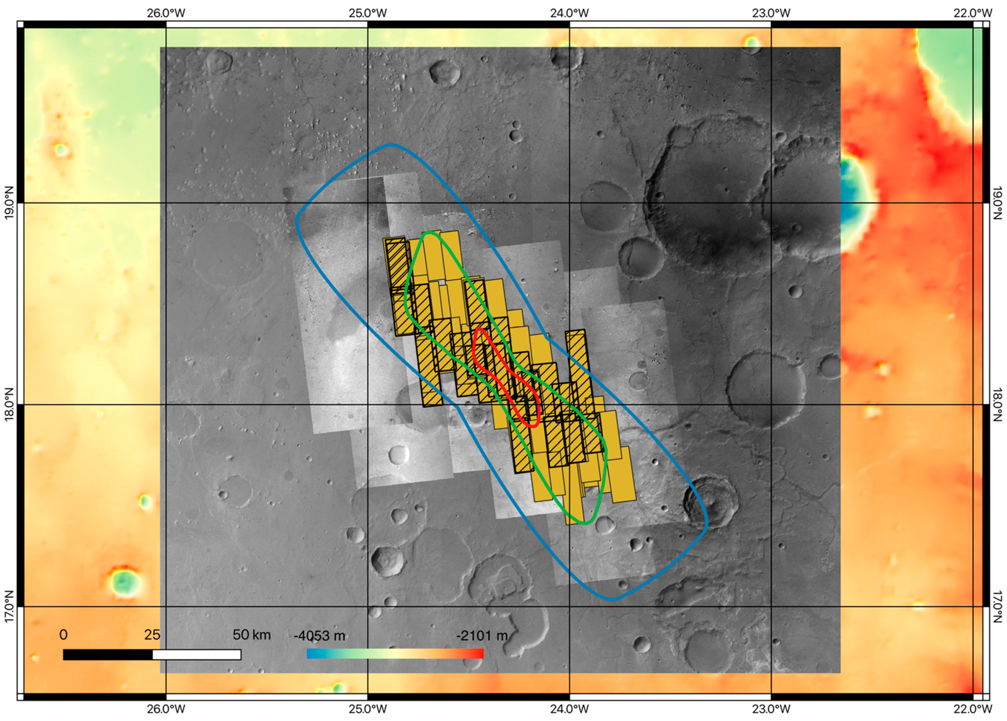
Figure 5.
1st row: Examples of a cropped area of the HiRISE MADNet DTMs—nine tiles mosaiced (A): insufficiently corrected against the reference DTM; (B): well-corrected against the reference DTM; (C): over-corrected against the reference DTM) and the CTX MADNet DTM mosaic (D): the reference DTM for A, B, and C; 2nd row: measured DTM profiles showing the difference between A, B, C, and D and the input CTX-co-registered HiRISE (ESP_037070_1985_RED) image.
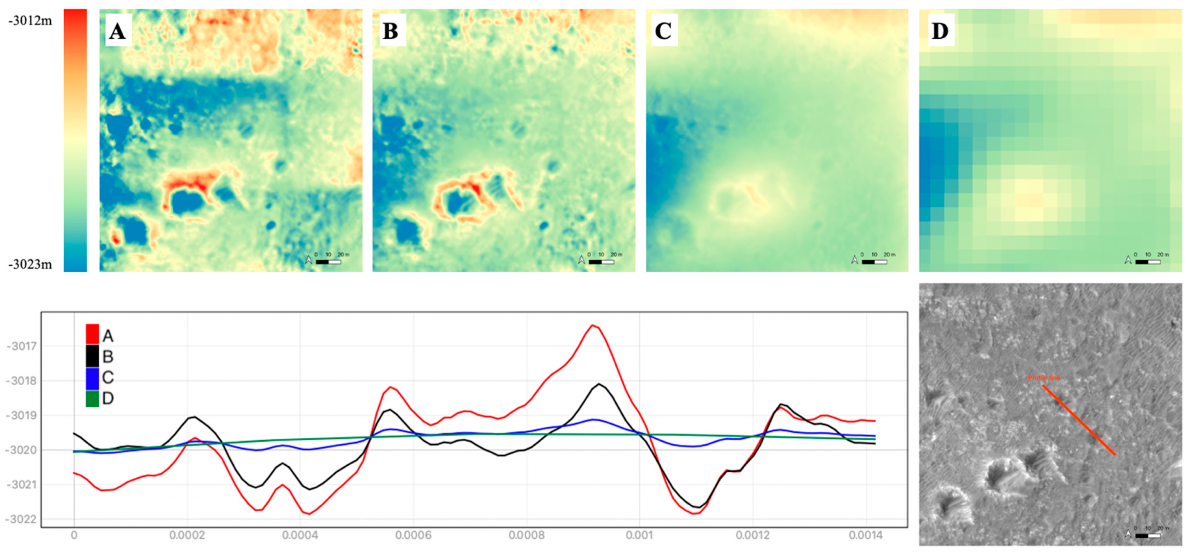
Figure 6.
Examples of the tiling artefact of the HiRISE (ESP_037703_1980_RED) MADNet DTM and the effect (including a measured profile crossing the tiling artefact) of using a larger number of overlapping pixels between each tile. It should be noted that the colourised DTMs and hill-shaded images show an identical area of interest. The profile location that is shown in the 1st row/2nd column is identical to the location of the measured profile in the 2nd row/2nd column.
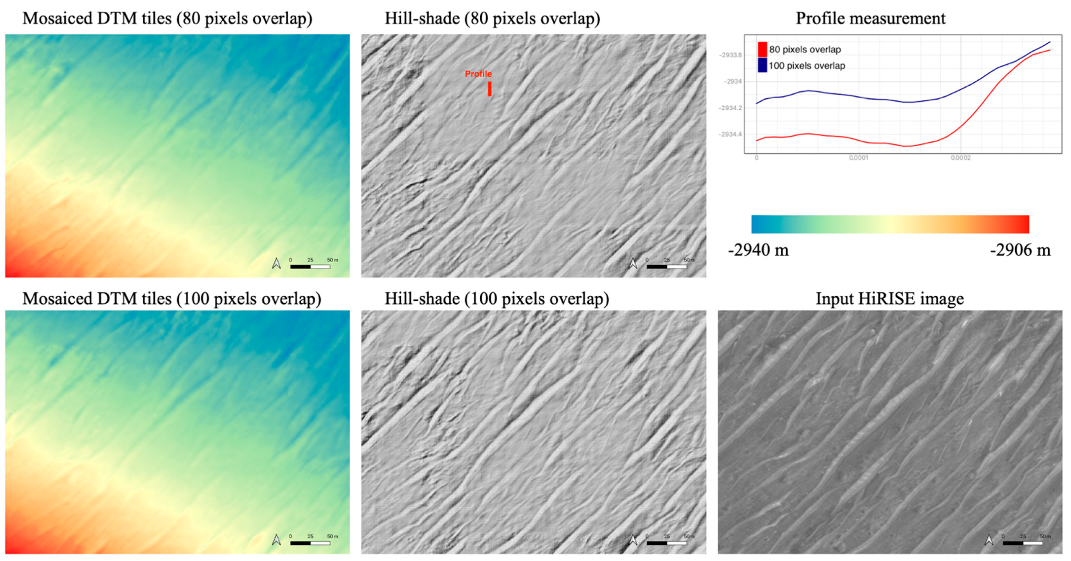
Figure 7.
The 25 m/pixel HRSC MADNet DTM mosaic (bottom row) compared to the 12.5 m/pixel HRSC MC-11W level 5 ORI mosaic (HMC_11W24_ND5, top row) and the 50 m/pixel HRSC MC-11W level 5 DTM mosaic (HMC_11W20_DA5, middle row). The 1st column shows the overview area, and the 2nd to 5th columns show the zoom-in views of four different areas (locations are labelled in top-left subfigure). Please refer to Supplementary Materials for each individual figure at full resolution.
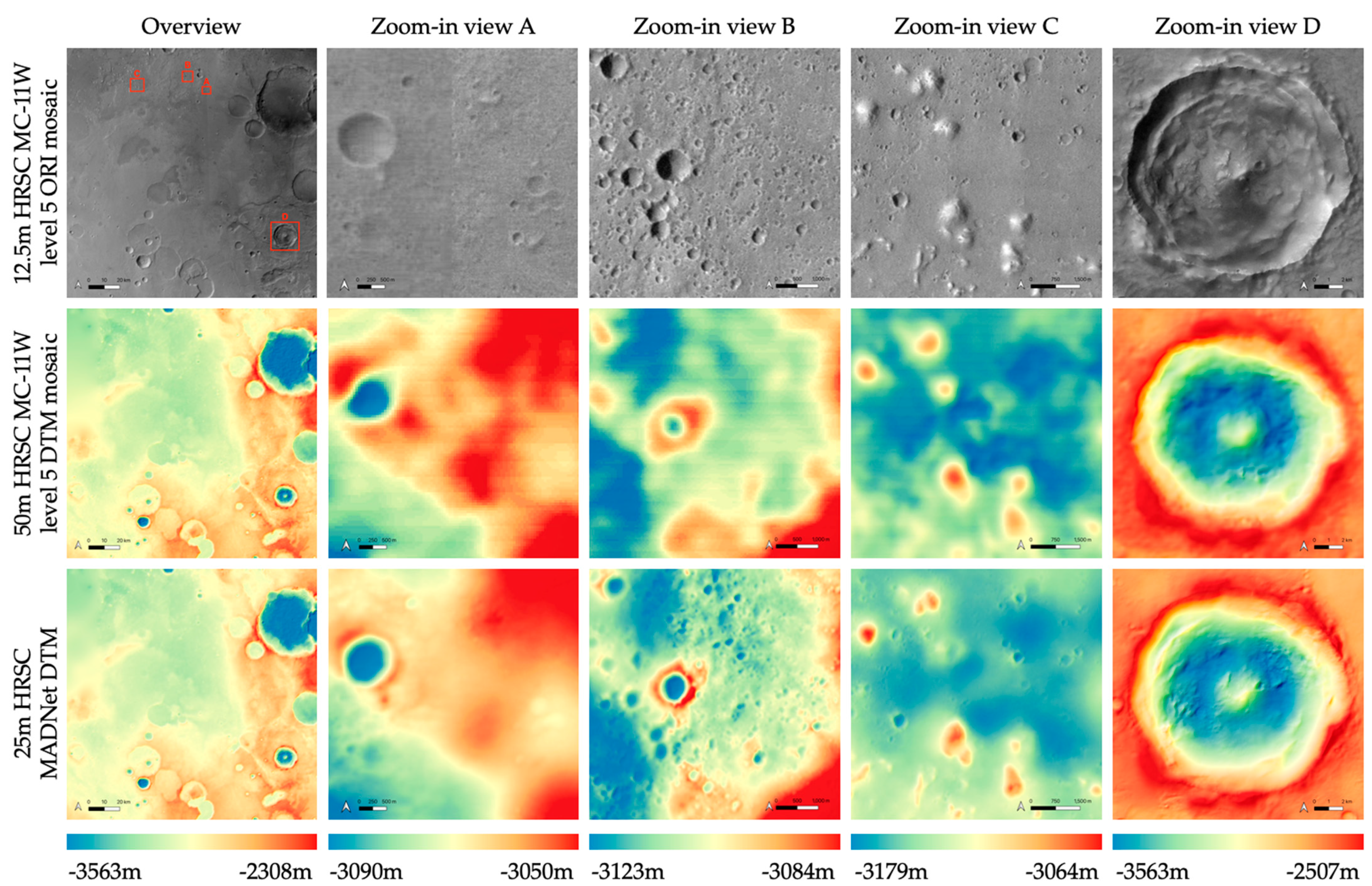
Figure 8.
Difference maps and scatter plots of the HRSC-to-MOLA comparisons (averaged) at the scale of 500 m/pixel for the original HRSC MC-11W level 5 DTM mosaic (HMC_11W20_DA5), the HRSC MC-11W level 5 DTM mosaic after 3D co-alignment, and the HRSC MADNet DTM mosaic. It should be noted that the mean and standard deviation (StdDev) are shown on the difference maps (1st row).

Figure 9.
The resultant 12 m/pixel CTX MADNet DTM mosaic in comparison to the 18 m/pixel CTX CASP-GO DTMs (photogrammetric results) and the 6 m/pixel CTX CASP-GO ORIs. The 1st column shows overviews of the ORIs and DTMs, and the 2nd to the 5th columns show the zoom-in views of four different areas (locations are labelled in the top-left subfigure from left-to-right). Please refer to Supplementary Materials for examination of each individual figure at full resolution.
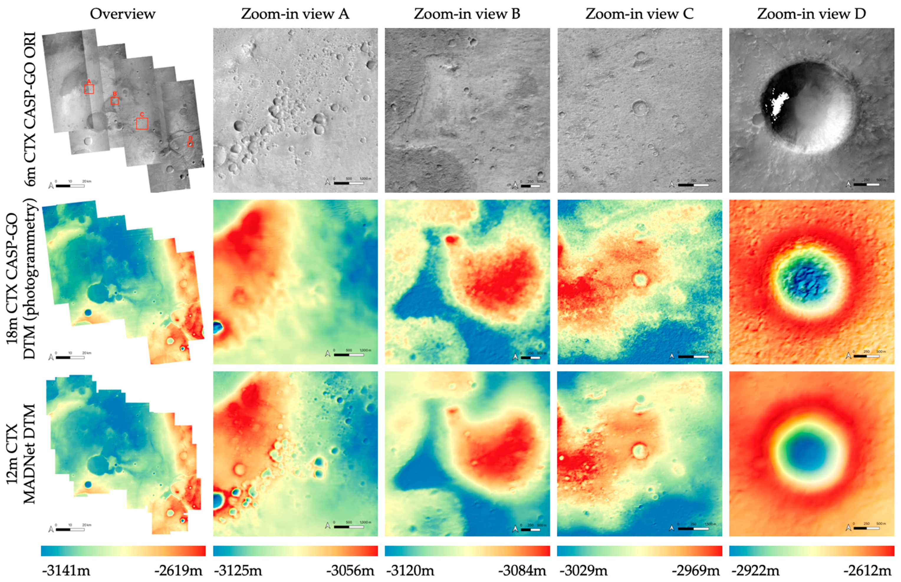
Figure 10.
Examples of the input CTX ORIs, before CTX-to-HRSC image co-registration (1st row) and after CTX-to-HRSC image co-registration (2nd row). The example CTX ORIs are in side-by-side views with the corresponding HRSC MC-11W level 5 ORI mosaic (1st and 3rd columns) and in side-by-side views with the neighbouring CTX ORIs (2nd and 4th columns).
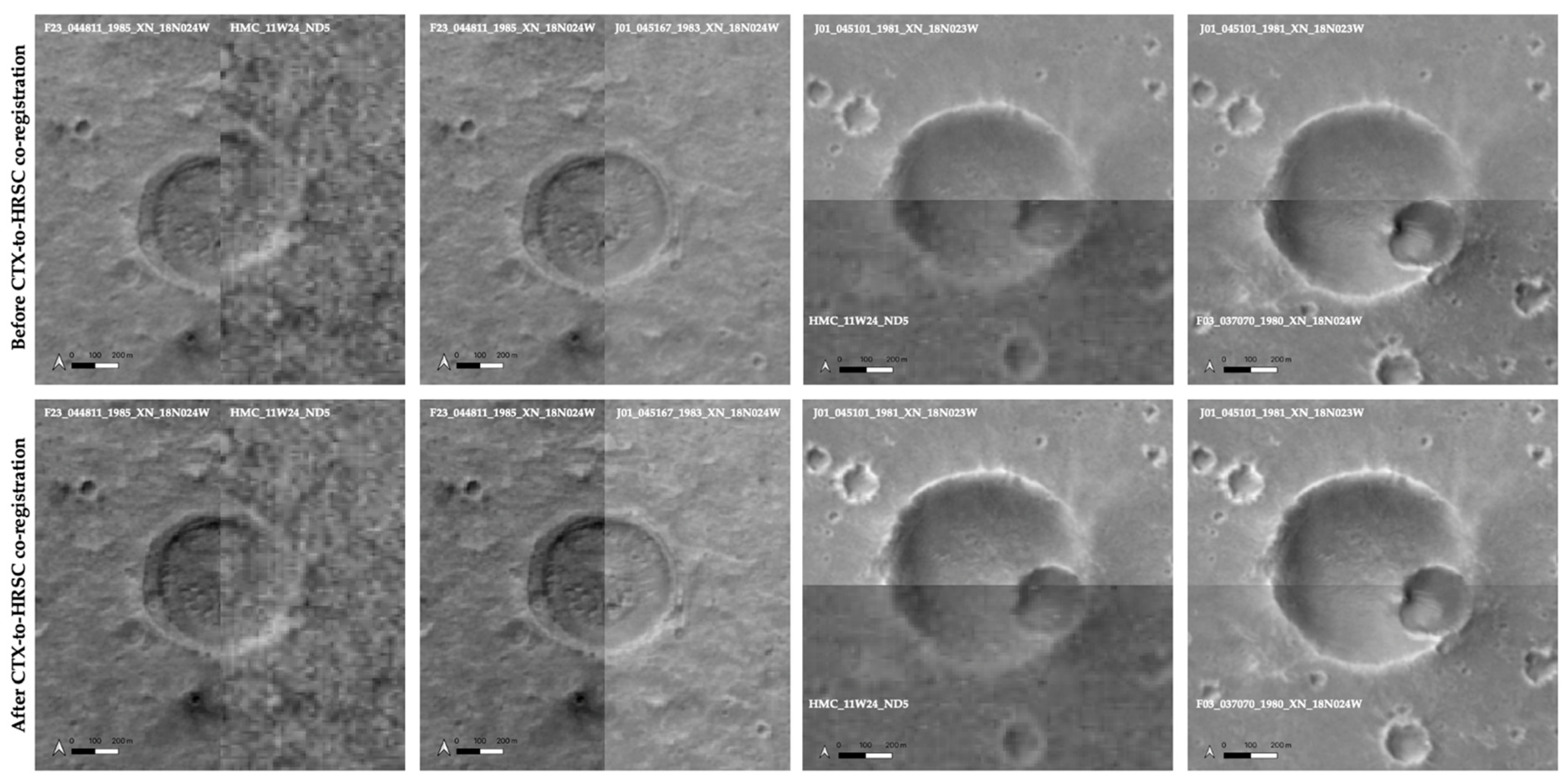
Figure 11.
Difference maps and scatter plots of the CTX-to-HRSC comparisons (averaged) at the scale of 50 m/pixel for (1st column) the CTX CASP-GO (photogrammetric) DTM mosaic (before 3D co-alignment), (2nd column) the CTX CASP-GO DTM mosaic (after 3D co-alignment), and (3rd column) the CTX MADNet DTM mosaic. It should be noted that the mean and standard deviation (StdDev) are shown on the difference maps (1st row).
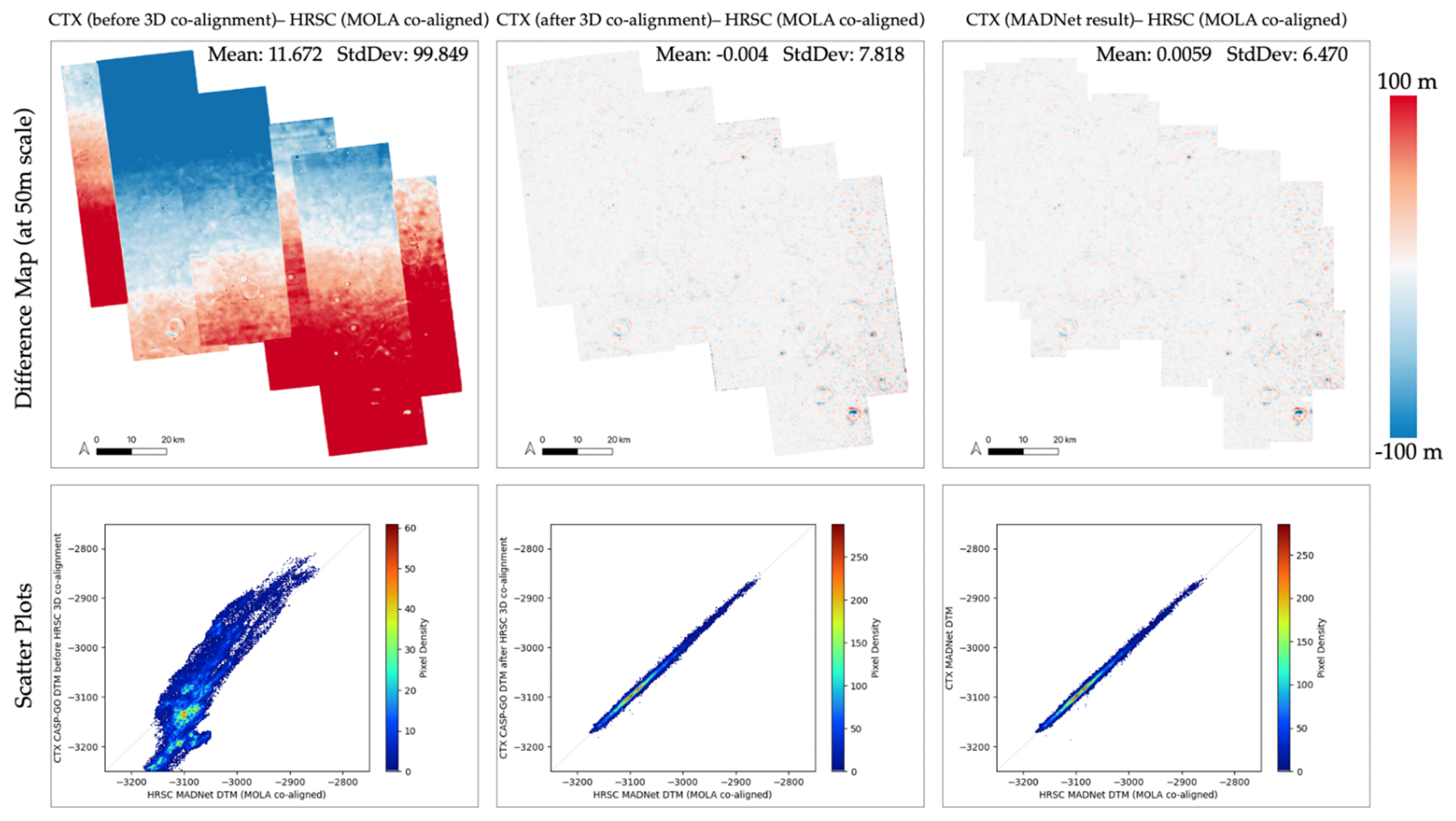
Figure 12.
The resultant 50 cm/pixel HiRISE MADNet DTM mosaic (consisting of 44 HiRISE MADNet DTMs) in comparison with the 1 m/pixel HiRISE PDS DTMs (photogrammetric results) and the 25 cm/pixel HiRISE ORIs. 1st row shows overviews of the ORIs and DTMs, and the 2nd to the 4th rows show the zoom-in views of six different areas (locations are labelled in the 2nd subfigure of the 1st row). Please refer to Supplementary Materials for details of each individual figure at full resolution.
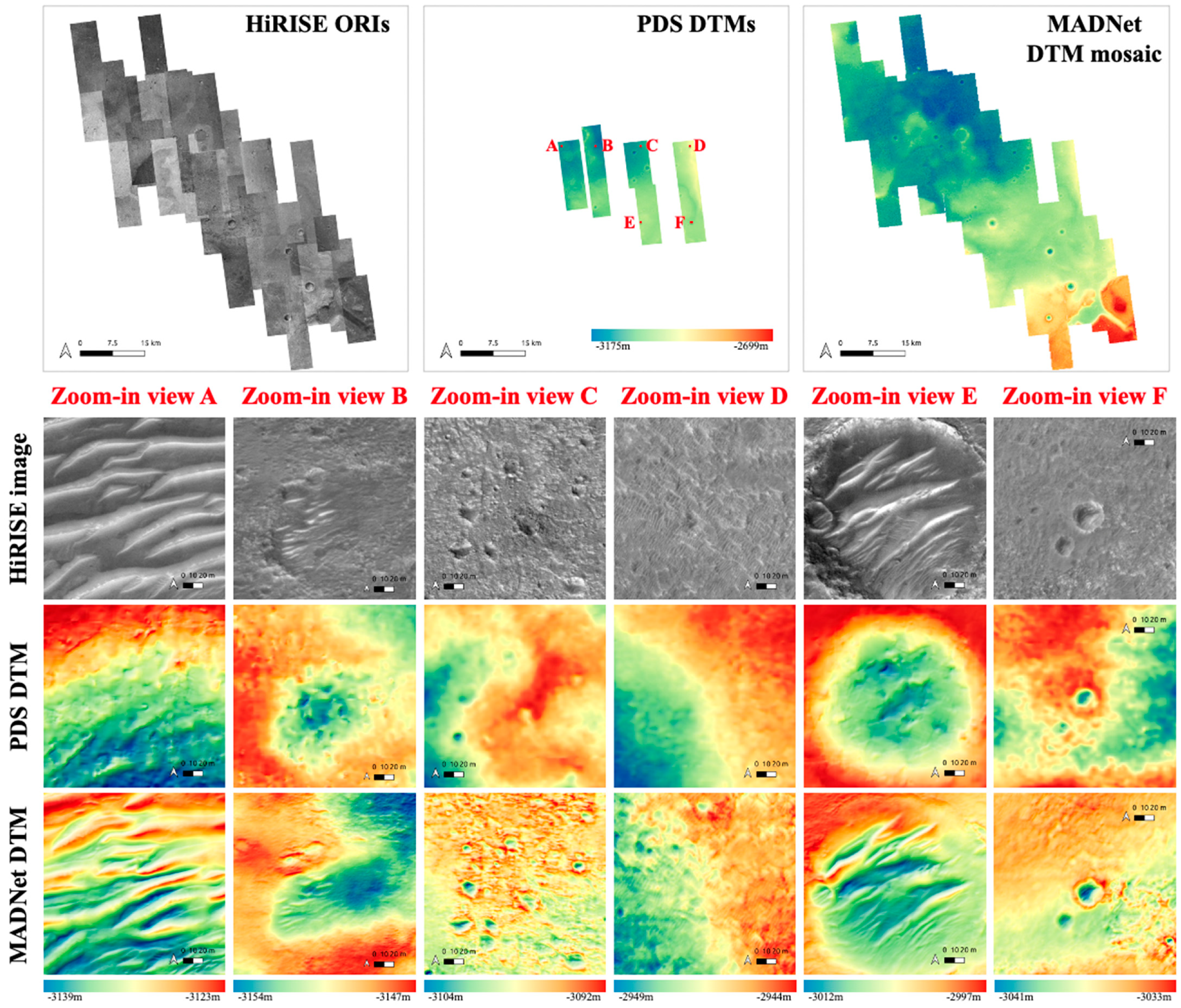
Figure 13.
Examples of the input HiRISE ORIs, before HiRISE-to-CTX image co-registration (1st row), and after HiRISE-to-CTX image co-registration (2nd row). The example HiRISE ORIs are in side-by-side views with the corresponding CTX ORIs (HRSC co-registered; 1st and 3rd columns) and in side-by-side views with the neighbouring HiRISE ORIs (2nd and 4th columns).
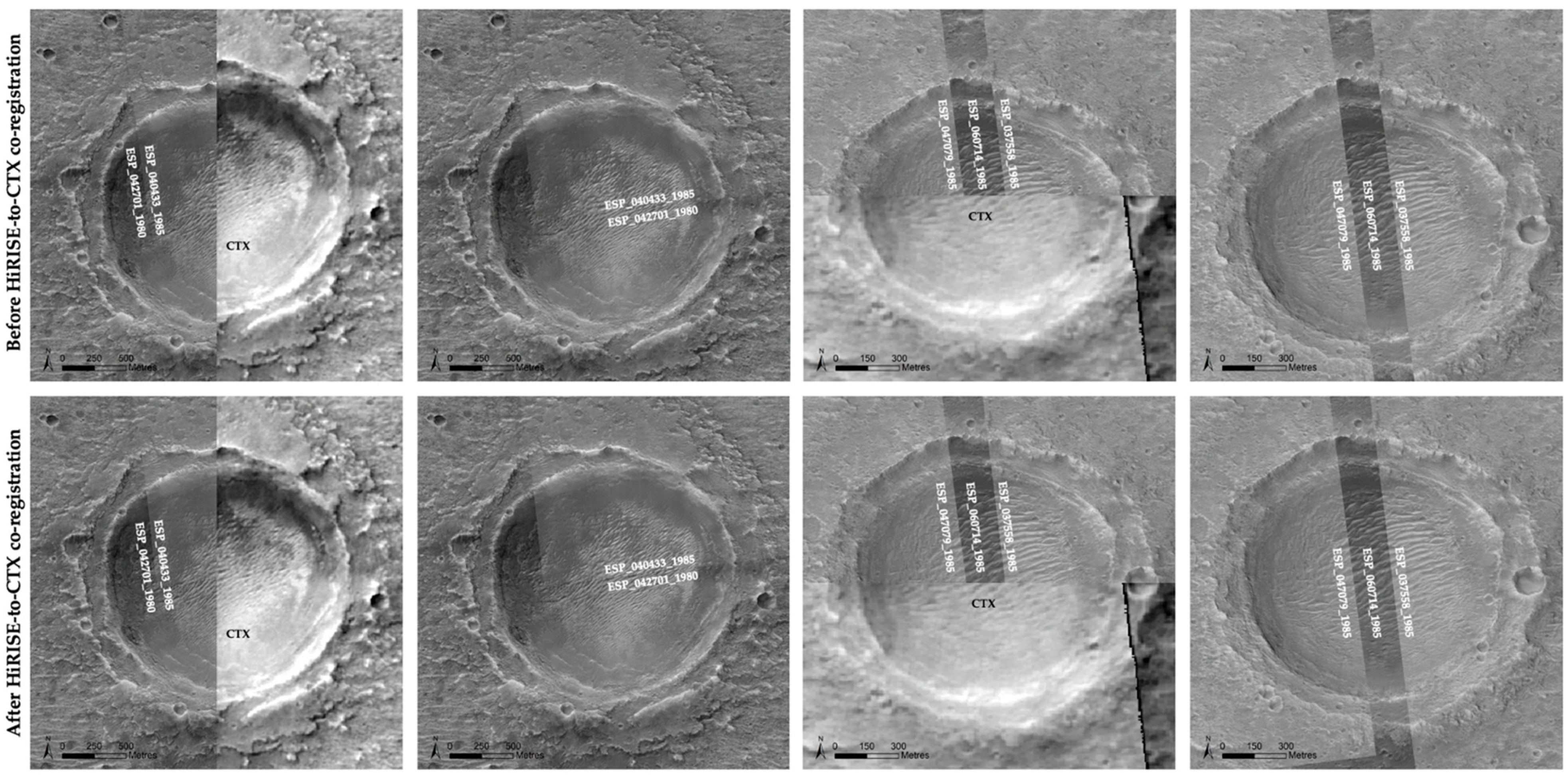
Figure 14.
Difference maps and scatter plots of the HiRISE-to-CTX elevation comparisons (averaged) at the scale of 12 m/pixel for the HiRISE PDS (photogrammetric) DTM mosaic and the HiRISE MADNet DTM mosaic. It should be noted that the mean and standard deviation (StdDev) are shown on the difference maps (1st row).

Figure 15.
Examples of the 25 cm/pixel HiRISE ORI (1st row), 50 cm/pixel HiRISE MADNet DTM mosaic (2nd row), and hill-shaded images (3rd–6th rows), using 45°, 135°, 225°, and 315°, of azimuth angles and 30° of illumination elevation with a vertical exaggeration factor of 3, of the resultant HiRISE MADNet DTM mosaic for four cropped areas (1st–4th columns) showing a large crater and small craters, layers, and hills.
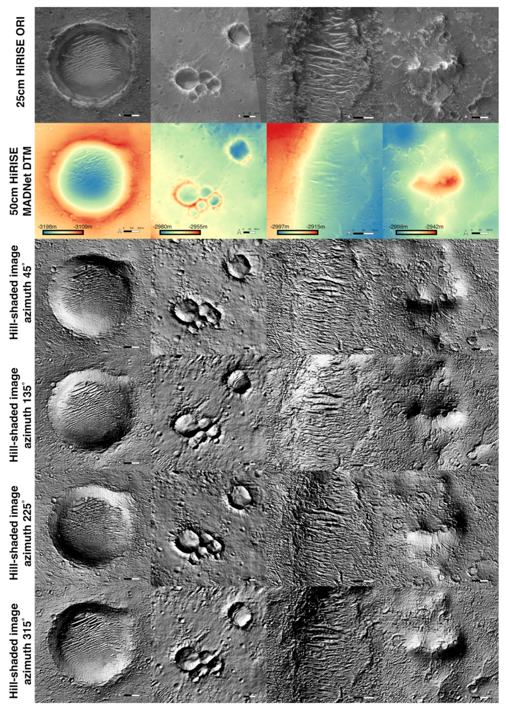
Figure 16.
Profile measurements of the resultant 50 cm/pixel HiRISE MADNet DTM mosaic, the 1 m/pixel HiRISE PDS DTM (DTEEC_003195_1985_002694_1985_L01), and the 12 m/pixel CTX MADNet DTM (co-aligned with HRSC/MOLA), using an example area with small-sized craters (from 10 m to 30 m diameter). The units of the y axis of all profile figures are in metres and the units of the x axis of all profile figures are normalised latitude and longitude degrees (counting from 0°). It should be noted that the MADNet DTM (2nd row) is colourised using the same colour key shown in the HiRISE PDS DTM (1st row). It should also be noted that the range of heights for Profiles 1–5 is a maximum of 14 m and that of Profiles 6–10 is 6 m.

Figure 17.
Examples of known artefacts of the HiRISE MADNet DTM mosaic, i.e., 1st column: tiling artefacts; 2nd column: smoothing issues; 3rd column: missing columns in the original HiRISE image; 4th column: linear artefacts due to the use of JPEG2000 HiRISE images that do not have the correct radiometric de-calibration. Hill-shaded image is created using the HiRISE MADNet DTM mosaic with illumination azimuth 330°, elevation 30°, and a vertical exaggeration factor of three times.


Table 1.
Input CTX image IDs (12 in total) that are co-registered and used as MADNet inputs.
| F03_037070_1980_XN_18N024W | J01_045101_1981_XN_18N023W | J05_046934_1985_XN_18N025W |
| F03_037136_1977_XN_17N023W | J02_045378_1981_XN_18N023W | F17_042622_1981_XN_18N024W |
| F23_044811_1985_XN_18N024W | J01_045167_1983_XN_18N024W | J14_050138_1986_XN_18N025W |
| F23_044956_1984_XN_18N024W | J03_045800_1983_XN_18N024W | K05_055518_1986_XN_18N025W |
Table 2.
Input HiRISE image IDs that are co-registered and used as MADNet inputs (44 images resulting in 44 HiRISE MADNet DTMs that are subsequently mosaiced to produce the final HiRISE MADNet DTM mosaic). N.B. left-to-right and top-to-bottom shows the order of the mosaicing priority.
Table 2.
Input HiRISE image IDs that are co-registered and used as MADNet inputs (44 images resulting in 44 HiRISE MADNet DTMs that are subsequently mosaiced to produce the final HiRISE MADNet DTM mosaic). N.B. left-to-right and top-to-bottom shows the order of the mosaicing priority.
| ESP_037558_1985_RED | ESP_037703_1980_RED | ESP_039154_1985_RED | ESP_039721_1980_RED |
| ESP_039932_1980_RED | ESP_040433_1985_RED | ESP_040921_1985_RED | ESP_042134_1985_RED |
| ESP_042701_1980_RED | ESP_044178_1985_RED | ESP_044257_1980_RED | ESP_044679_1985_RED |
| ESP_047079_1985_RED | ESP_047435_1985_RED | ESP_047501_1985_RED | ESP_049927_1980_RED |
| ESP_051272_1985_RED | ESP_052828_1980_RED | ESP_055175_1980_RED | ESP_055241_1980_RED |
| ESP_057747_1985_RED | ESP_058090_1985_RED | ESP_058169_1985_RED | ESP_059659_1980_RED |
| ESP_059725_1985_RED | ESP_060714_1985_RED | ESP_066833_1980_RED | ESP_067044_1990_RED |
| ESP_067585_1990_RED | ESP_068258_1980_RED | ESP_068456_1985_RED | PSP_003195_1985_RED |
| PSP_007019_1980_RED | PSP_009735_1985_RED | ESP_037070_1985_RED | ESP_046512_1980_RED |
| ESP_051206_1985_RED | ESP_019084_1980_RED | ESP_043268_1980_RED | ESP_062402_1985_RED |
| ESP_065448_1985_RED | ESP_067717_1985_RED | PSP_002694_1985_RED | ESP_045167_1980_RED |
Publisher’s Note: MDPI stays neutral with regard to jurisdictional claims in published maps and institutional affiliations. |
© 2021 by the authors. Licensee MDPI, Basel, Switzerland. This article is an open access article distributed under the terms and conditions of the Creative Commons Attribution (CC BY) license (https://creativecommons.org/licenses/by/4.0/).
Share and Cite
MDPI and ACS Style
Tao, Y.; Muller, J.-P.; Conway, S.J.; Xiong, S. Large Area High-Resolution 3D Mapping of Oxia Planum: The Landing Site for the ExoMars Rosalind Franklin Rover. Remote Sens. 2021, 13, 3270. https://doi.org/10.3390/rs13163270
AMA Style
Tao Y, Muller J-P, Conway SJ, Xiong S. Large Area High-Resolution 3D Mapping of Oxia Planum: The Landing Site for the ExoMars Rosalind Franklin Rover. Remote Sensing. 2021; 13(16):3270. https://doi.org/10.3390/rs13163270
Chicago/Turabian StyleTao, Yu, Jan-Peter Muller, Susan J. Conway, and Siting Xiong. 2021. "Large Area High-Resolution 3D Mapping of Oxia Planum: The Landing Site for the ExoMars Rosalind Franklin Rover" Remote Sensing 13, no. 16: 3270. https://doi.org/10.3390/rs13163270
Note that from the first issue of 2016, this journal uses article numbers instead of page numbers. See further details here.