Article

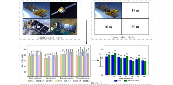
How Spatial Resolution Affects Forest Phenology and Tree-Species Classification Based on Satellite and Up-Scaled Time-Series Images

1
School of Resources and Environmental Engineering, Hefei University of Technology, Hefei 230009, China
2
Institute for Spatial Information Intelligence Analysis and Application, Hefei University of Technology, Hefei 230009, China
3
Intelligent Interconnected Systems Laboratory of Anhui Province, Hefei 230009, China
4
International Institute for Earth System Science, Nanjing University, Nanjing 210023, China
5
College of Information and Management Science, Henan Agricultural University, Zhengzhou 450002, China
*
Author to whom correspondence should be addressed.
Remote Sens. 2021, 13(14), 2716; https://doi.org/10.3390/rs13142716
Submission received: 11 May 2021 / Revised: 1 July 2021 / Accepted: 7 July 2021 / Published: 10 July 2021
(This article belongs to the Special Issue Mapping Tree Species Diversity)

Abstract

:
The distribution of forest tree species provides crucial data for regional forest management and ecological research. Although medium-high spatial resolution remote sensing images are widely used for dynamic monitoring of forest vegetation phenology and species identification, the use of multiresolution images for similar applications remains highly uncertain. Moreover, it is necessary to explore to what extent spectral variation is responsible for the discrepancies in the estimation of forest phenology and classification of various tree species when using up-scaled images. To clarify this situation, we studied the forest area in Harqin Banner in northeast China by using year-round multiple-resolution time-series images (at four spatial resolutions: 4, 10, 16, and 30 m) and eight phenological metrics of four deciduous forest tree species in 2018, to explore potential impacts of relevant results caused by various resolutions. We also investigated the effect of using up-scaled time-series images by comparing the corresponding results that use pixel-aggregation algorithms with the four spatial resolutions. The results indicate that both phenology and classification accuracy of the dominant forest tree species are markedly affected by the spatial resolution of time-series remote sensing data (p < 0.05): the spring phenology of four deciduous forest tree species first rises and then falls as the image resolution varies from 4 to 30 m; similarly, the accuracy of tree species classification increases as the image resolution varies from 4 to 10 m, and then decreases as the image resolution gradually falls to 30 m (p < 0.05). Therefore, there remains a profound discrepancy between the results obtained by up-scaled and actual remote sensing data at the given spatial resolutions (p < 0.05). The results also suggest that combining phenological metrics and time-series NDVI data can be applied to identify the regional dominant tree species across different spatial resolutions, which would help advance the use of multiscale time-series satellite data for forest resource management.

Graphical Abstract

1. Introduction

Accurate spatial distribution information of forest tree species is a precondition for almost all questions dealing with regional forest ecology and is quite important for understanding the land-surface phenology (LSP) processes and the refinement of ecological and atmospheric models [1,2,3]. In addition, accurate mapping of the dominant tree species is critical for forest-environment monitoring, forest management, and associated decision-making and planning [4,5]. In recent years, remote sensing images with medium to high spatial resolution (≤30 m) have been widely used to map and classify dominant tree species in the different regional forest ecosystems, because the viewing field of the image is close to the size of tree species and of tree stands [6,7,8,9]. However, given the limitations to a few bands with wide central bandwidths, it remains challenging to map forests finely and accurately by solving the common problem of foreign bodies with spectra similar to that of tree species with multispectral images of differing resolution [10,11,12,13].
With today’s continuous improvement in multispectral satellite revisit cycles, temporal characteristics have proven to have high application value for forest classification [14,15]. The time-series normalized differential vegetation index (NDVI) was generally considered to be applicable for identifying vegetation and extracting phenological information [16,17,18], which plays a key role in classifying the dominant tree species and overcoming the problem of foreign bodies with similar spectra [19,20]. Given this advantage, some studies have confirmed the use of time-series NDVI data and phenological characters would raise the mapping accuracy of forest types in both urban areas [13,21] and rural areas [18,22,23,24].
MODIS and NOAA satellites can provide images with very short revisit intervals (less than 2 days). Therefore, most previous researches have discussed the results of forest composition mapping and dynamic detection based on time-series NDVI data from a regional to global scale [5,25]. However, the spatial resolution of traditional time-series images such as NOAA AVHRR [26], SPOT Vegetation [27], and MODIS imagery data [28] generally range from hectometers to kilometers, resulting in poor spectral purity and limited identification of broad forest types (such as coniferous or broad-leafed forests). Hence, medium-to-low resolution remote sensing images were considered to be applicable to classify general forest-cover types [29,30] in which finer tree species composition information is not involved [9,31]. As a rule, medium-high resolution satellite images can be used to produce more accurate results of forest species composition by providing detailed spectral features of the canopy of dominant tree species [32,33].
An increasing number of medium- and high-resolution Earth-observation satellites have now entered use in recent years (e.g., Sentinel-2, SPOT-6 and -7, Gaofen-1 and -2, etc.). Some multitemporal medium-high-resolution NDVI images have proven to be applicable to classify the dominant tree species in forests [11,34,35,36], but less attention has been focused on spatial mapping [37]. In addition to the time-series spectral dynamics, plant phenology should be equally considered for tree species mapping [38,39,40,41]. Therefore, it is essential to use multiscale time-series data to explore the effect of image resolution and phenology information on the accuracy of forest tree species classification. The study of vegetation-phenology dynamics by remote sensing mainly involves extracting the corresponding key time nodes and characteristic values by analyzing the significant variations in vegetation index time series data, which are commonly called LSP metrics [11,17,42,43]. LSP metrics are important status parameters for land-vegetation ecosystems, especially at the start of spring (SOS) [44], also called the start of the growing season [45] or the green-up date [46]. These parameters are the most commonly extracted because of their importance in determining the growing season, and they are also powerful indicators of an ecosystem’s response to climate change [44].
To date, LSP metrics have been used to identify different vegetation species. For example, Liu et al. (2018) used the combination of fused 30 m time-series NDVI data and phenological metrics to map rice paddies, and they found that using both of the selected NDVI and phenological features could allow the highest accuracy in extracting rice paddy areas [47]. Another recent study suggested that phenological metrics can help improve the accuracy of remote-sensing recognition of different forest stands [17]. In addition, Schwieder et al. (2018) demonstrated that adding phenological information from multitemporal imagery improves the estimation of aboveground biomass through modified discrimination of vegetation types [48]. However, few studies involving the mapping and phenology of forest tree species have integrated different spatial observation scales with multiscale satellite images, which is necessary to compensate for the lack of research on higher-resolution time-series data.
The mapping results of forest types or tree species through remote sensing would be influenced by the spatial resolution of remote sensing data obviously [6,7,49,50]. In addition, most previous studies have focused on single time-phase imagery, which led to no results available on temporal data [51]. In fact, both species classification and phenological metrics are affected by the spatial resolution of remote sensing data. For example, Zhang et al. (2017) explored how spatial resolution affects the start of vegetation season (SOS) by comparing observations obtained from images with 30 m and 500 m spatial resolution, and found the difference of SOS at the high and low resolution was larger in heterogeneous regions [52]. Tian et al. (2020) investigated how spatial resolution affects the difference in spring phenology of rural-urban vegetation as detected by resampling the satellite data from 30 m to 8 km spatial resolution. They found that coarser images overestimate the urbanization effects and that the SOS obtained by coarser time-series NDVI data would be earlier than that of the actual result [53]. It should be noted that the multiresolution imagery data used in the above researches consists of resampled multispectral images by using up-scaled algorithms (e.g., Nearest Neighbor (NN) and pixel aggregation (PA)), which generate a set of lower spatial resolution images using the high-resolution image through pixel resampling. However, the imaging mechanism of these up-scaled images differs from that of satellite imagery data obviously, which may lead to some uncertainty in the final results of relevant studies [51,54,55]. In consequence, it could be assumed that the phenological monitoring results obtained by up-scaled time-series NDVI data may differ from that detected from time-series satellite imagery, which accounts for the necessity to re-evaluate the results associated with time-series resampled images [53].
In this study, we systematically evaluate how temporal images with a medium-high spatial resolution (4, 10, 16, and 30 m) affect the accuracy of forest tree species mapping and the variability of spring phenological information. The multiscale time-series satellite remote sensing data were obtained from Gaofen-2 (4 m), Sentinel-2 (10 m), Gaofen-1 (16 m), and Landsat-8 (30 m), respectively, acquired over seasonal deciduous forests in 2018 from a state forest farm region in Harqin Banner, China. In addition, we evaluate the performances obtained by using up-scaled time-series images of different spatial resolutions. Eight phenological metrics are extracted to classify forest tree species based on the random forest (RF) algorithm combined with time-series NDVI data. Accordingly, we tried to find out (1) what is the regular pattern for monitoring spring phenology within the medium-high remote sensing spatial resolution range; (2) which scales of time-series images most effectively reflect spectral differences in each forest tree species and the relationship between these phenological metrics and tree species classification; and (3) whether the spatial patterns in up-scaled images are competitive to map the distribution of forest tree species from multiscale satellite datasets. Answers to these points should improve the credibility of using time-series remote sensing images to monitor and map forest tree species for use in forest resource management or regional eco-climate models.

2. Materials and Methods
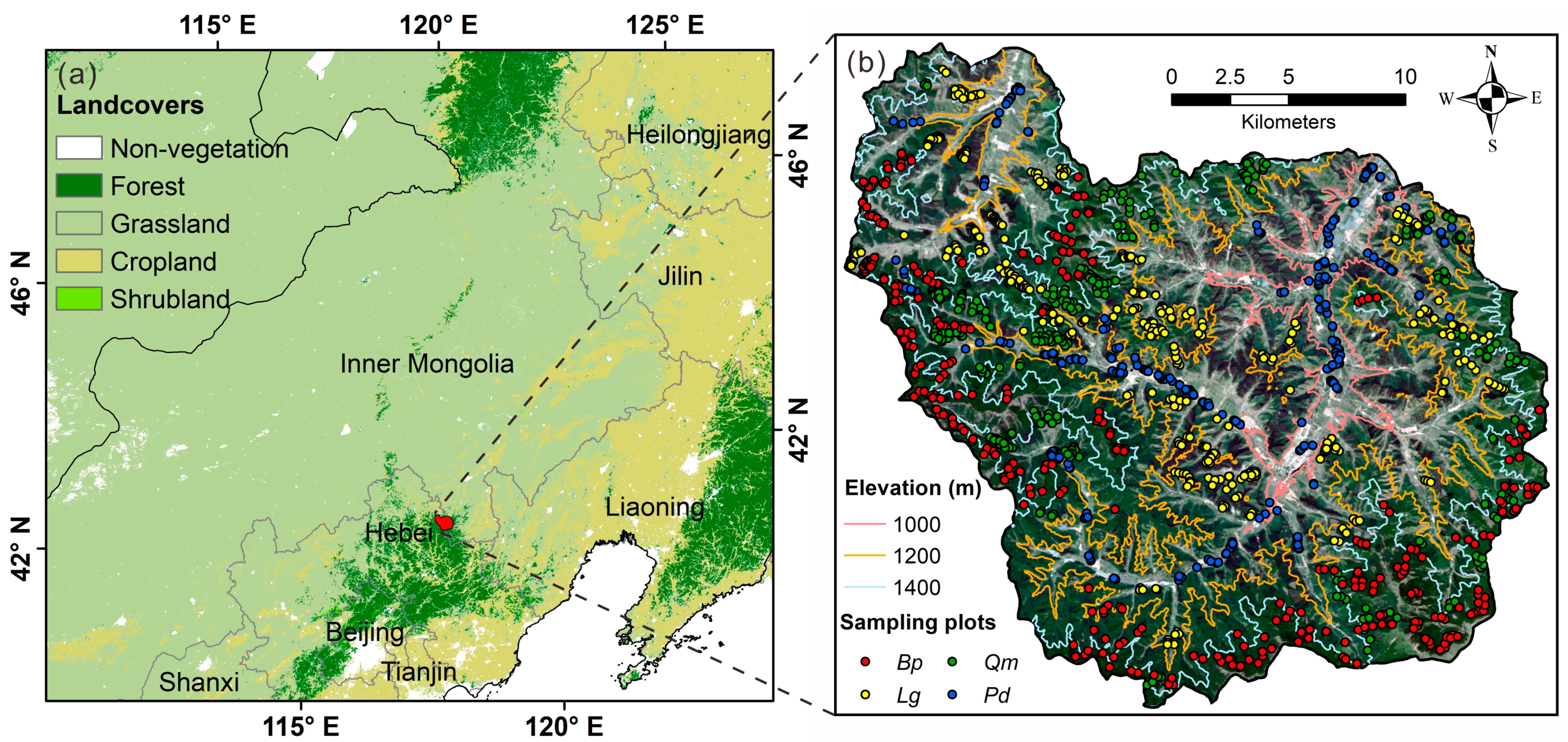
2.1. Study Area

The study area is in northeast China near the city of Chifeng and has a size of approximately 55,100 ha of which over 45,500 ha are forested landscape. An overview of the area is given in Figure 1. The study area belongs to the border area of the Greater Hinggan Mountains and Yanshan Mountains within a range of 878 to 1890 m, and the climate here is temperate monsoon. The dominant tree species occurring in the local forest are deciduous forest dominated by Quercus mongolica (Qm), Populus davidiana (Pd), Betula platyphylla (Bp), and Larix gmelinii (Lg), accounting for about 84% of the total forest area in 2018; there is also an evergreen forest, which is dominated by Pinus tabulaeformis (Pt). The five dominant tree species mentioned above account for over 95% of the total forest area in 2018 [19].

2.2. Methods

The methodological workflow is illustrated by the flowchart presented in Figure 2. The research process includes four main steps. First, the collection and preprocessing of both remote sensing data and ground observation data were completed. Next, we calculated forest phenological metrics based on multiscale time-series data and analyzed the scale effect of spring phenology. Then, forest tree-species mapping was performed using satellites and up-scaled time-series NDVI data and phenological metrics with different spatial resolutions. Finally, comparisons of multiple considerations on the accuracy of forest mapping were conducted to illustrate how spatial resolution affects tree-species classification.

2.2.1. Data Resources and Preprocessing

We selected four sets of multiresolution remote sensing images acquired once per month to make a series of spatial scale images respectively (Table A1 in Appendix A) and acquired with cloudiness less than 15%. The main parameters of the images used in this study can be seen in Table 1. This study used a total of 48 satellite remote sensing images covering the entire study area; there were 46 of them acquired in 2018 while the other two with poor imaging quality were replaced by the data of the same period in 2017, which was proven to be feasible [19]. All Sentinel-2 images were obtained from the European Space Agency (ESA; https://scihub.copernicus.eu; accessed on 18 December 2019); Landsat-8 images were obtained from the United States Geological Survey (USGS; http://glovis.usgs.gov; accessed on 15 January 2020); Gaofen-1 and Gaofen-2 images were obtained from the China Center for Resources Satellite Data and Application (CCRSDA; http://www.cresda.com/CN; accessed on 12 September 2020).
Before analysis, the four sets of time-series datasets with different spatial resolutions were carefully harmonized. A Savitzky–Golay (SG) algorithm served for polynomial filtering of the time-series NDVI data because it better maintains the temporal vegetation dynamics and minimizes atmospheric effects [56,57]. This also implied a smoothing and filtering of the four time-series could remove undesired artifacts due to poor atmospheric conditions and undetected clouds [58]. The four sets of multiscale time-series data preprocessing by using a series of related models and algorithms in ENVI (Environment for Visualizing Images; version 5.3) and IDL (Interactive Data Language; version 8.5) software platform (Research Systems Inc., Boulder, CO, USA). The orthorectification, atmospheric radiation correction, and geometrical rectification were carried out in sequence to preprocess all images used in this study, to transform the digital value into the actual surface spectral reflectance at different image resolutions (Figure 2). The radiometric correction methods include the incident causational matrix (ICAM), and pseudo-invariant feature (PIF) models [59], and the corresponding parameters of radiation correction of different satellite remote sensing data were obtained from their official websites, that is CCRSDA, ESA, and USGS, respectively. In addition, the geometric root means squared error (RMSE) of all images was controlled within 0.5 pixels.
The PA algorithm was selected for up-scaled images (Figure 2). PA assigns different weights to each pixel based on mapping distance which is integrated at the ENVI software, and it is widely used in researches of multiscale remote sensing [46,53]. One related study suggests that PA better maintains pixel values than do other up-scaled algorithms (e.g., nearest neighbor, bilinear, and cubic convolution) [51]. The NDVI data then were calculated as Equation (1). To ensure that different time series can be compared to each other, the up-scaled datasets were smoothed in the same way as the satellite data. To better analyze the timing of (phenological) events, the (smoothed) monthly NDVI series were saved as 30 daily values on the 15th of each month were assigned as DOY (day of the year; Julian date) for the compositing period of the month.
NDVI = ρ NIR ρ red ρ NIR + ρ red
where ρNIR and ρred are the surface reflectance of near-infrared (NIR) and red bands.

2.2.2. Collection of Forest Inventory Data

The field surveys in the study area were undertaken in July 2018 and May 2019. A total of 1320 sample plots (30 m× 30 m) were selected randomly. Approximately 330 sample sites for each deciduous dominant tree species (Table A2 in Appendix A) are shown in Figure 1 (more than 85% of the tree population is single species). Then, 70% of these data were randomly set as training samples and the rest as verification samples. Therefore, the spectral reflectance of different dominant tree species was extracted from the center of each stand plaque at each sample point in the imagery to guarantee the spectral purity of the different image pixels.

2.2.3. Calculation of Forest Phenological Metrics

From the time series NDVI images with different spatial resolutions for related functions in TIMESAT [60], eight typical phenological metrics were obtained: the start of growth season (SOS), end of growth season (EOS), length of growth season (LOS), peaking time of growth season (POS), length of the peak-time (LOP), middle of SOS (SOSm), middle of EOS (EOSm), and amplitude (AMP). All the mentioned phenology-related metrics are noted as the Julian date. Here, both the SOS and EOS were calculated from the fitting function when the trees grow to a certain fixed time phase, e.g., the time position ranges from the position where 10–30% of the left (right) minimum of the NDVI value and the maximum NDVI value [61,62], which was indicated as a suitable time point. Nevertheless, the threshold of the determined phenological time points ranged around 20% according to the geographical locations and tree species selected [19,63,64]. The LOS is further calculated as the difference between the EOS and SOS, the POS is identified as the date when the trees grew to the maximum NDVI value at the fitted temporal dynamic curve, then the LOP is the length between 80% of the left and right maximum NDVI of the temporal dynamic curve. The amplitude (AMP) presents the maximum ranges of the tree photosynthetic dynamics across the whole growing season, and SOSm and EOSm stand for the average days of the growing season when the trees grow above their 80% level on the right and left side of the peaking time. A more detailed description of the calculated metrics can be found in Schwieder et al. (2018) [48] and Lebrini et al. (2019) [65].

2.2.4. Classification and Accuracy Assessment

Supervised classifiers are believed to be more clearly preferable while the prior knowledge for ground objects is enough [66]. In this study, we used the Random Forest (RF) classifier to identify deciduous tree species, and set its ntree to 500 and the mtry to the square root of the number of input features, as suggested [67,68,69]. RF is derived from statistical learning theory to process high-dimension datasets and reduce the overfitting issues [69,70,71], which was considered to be one of the most robust classifiers compared with other algorithms, such as maximum likelihood (ML), linear discriminant analysis (LDA), support vector machine (SVM), and decision tree classifiers (DTC) [72,73,74]. Therefore, it integrates hundreds of decision-making trees and encapsulates an important ranking predictor (the mean decreases of accuracy; MDA), which was designed to be used to evaluate the importance of variables in the accuracy efficiently [75]. Then, we extracted the forest boundary and used winter images to separate the dominant evergreen forest landscape. Based on this, we focused on the remote-sensing classification results for the four deciduous forest tree species: Betula platyphylla (Bp), Populus davidiana (Pd), Quercus mongolica (Qm), and Larix gmelinii (Lg) based on time-series NDVI data and the combination of NDVI and phenological metrics.
In addition, we calculate the overall accuracy (OA), kappa, and the accuracies of producer and user to examine and compare each result from different image datasets by constructing corresponding error matrices [76]. By randomly selecting training samples and validation samples, each set of classification results was cross-validated 10 times and averaged. The one-way analysis of variance (ANOVA) was used to decide significant differences in the classification results among the different spatial resolutions and methods. This was followed by multiple comparisons using the least-significant difference (LSD) to identify where the differences lay (p < 0.05).

3. Results

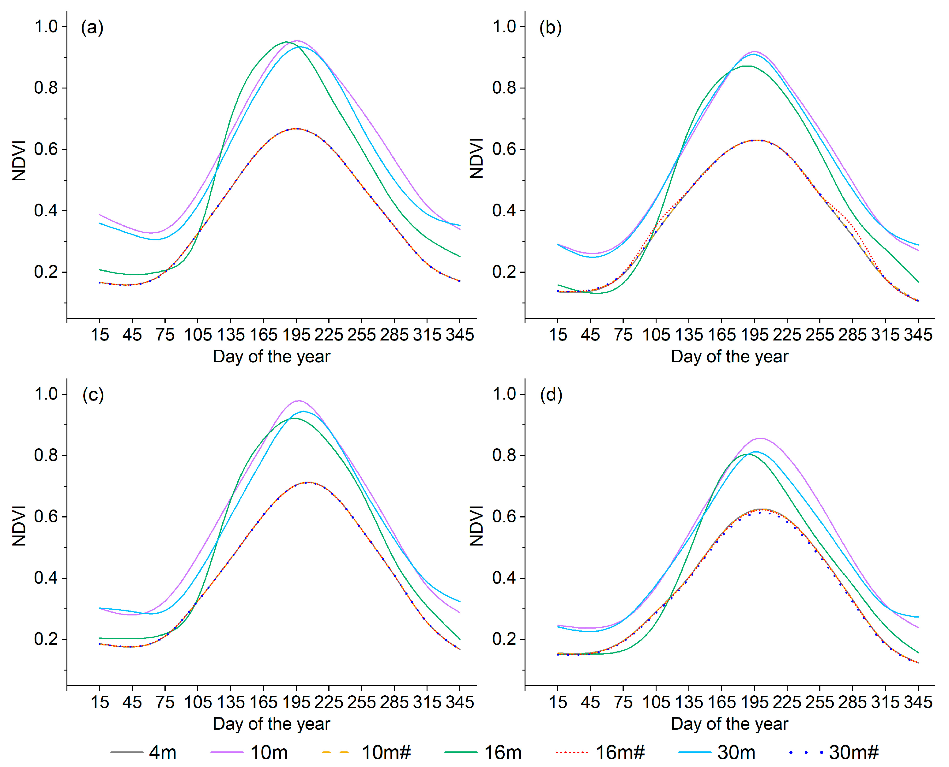
3.1. Multiscale Sequence NDVI Curve of Different Deciduous Forest Stands

The annual NDVI curves of the four deciduous forest species with spatial resolution range from 4 to 30 m show obvious unimodal characteristics, with clear forest stand growth stage characteristics (Figure 3). However, the mean NDVI values of four dominant deciduous tree species in the study area were significantly different, in especial, the spectral reflectance captured in 4 m high-resolution images is significantly less than that in lower-spatial-resolution images (p < 0.05). In addition, the NDVI curves of different dominant tree species differ, where the NDVI curve of Qm is higher than that of the other deciduous tree species, and that of Pd is the lowest.
In terms of the up-scaled NDVI curves, there are no significant changes in almost all NDVI data observed (p > 0.05), which is significantly below the NDVI value from multiscale satellite images at each given spatial resolution (p < 0.05), meaning the up-scaled NDVI curves were underestimated compared to that obtained from actual satellite data at the same resolution.

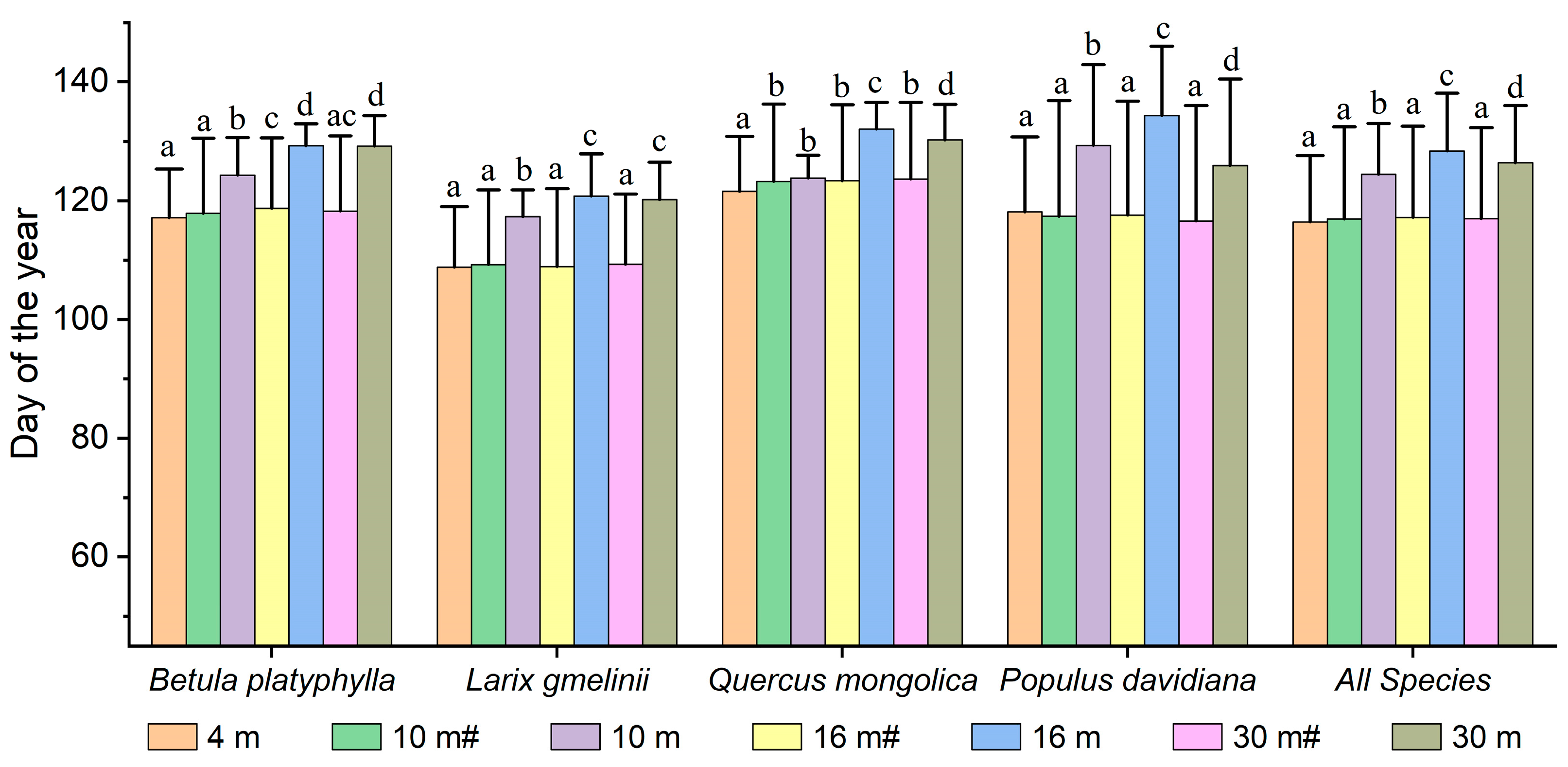
3.2. Multiscale SOS Results by Satellite Images

The SOS results of multiscale images of different dominant tree species differ significantly (p < 0.05; Figure 4). For different tree species, the mean SOS for Lg (109–121) is the earliest, Bp (117–129) is relatively later than all species (including four deciduous tree species; 116–128), and Pd (118–134) is slightly earlier than Qm (122–132), showing the phenological difference among the four deciduous tree species in this study region. For different spatial resolutions, almost all dominant deciduous tree species reveal a significant difference in the mean SOS based on native multiscale images at the same spatial resolution from 4 to 30 m (p < 0.05). Overall, the mean SOS increases from 4 to 16 m and then decreases slightly to 30 m (p < 0.05). Similarly, the SOS results of all species first increase and reach a peak at 16 m resolution and then begin to decrease as the resolution comes to 30 m (p < 0.05), where the mean SOS delay time ranges from 8.02 to 11.95 days.
However, the SOS results for each tree species at different up-scaled spatial resolutions are similar relatively, and an analysis of variance demonstrates that no significant difference appears between image resolutions from 4 to 30 m (p > 0.05), whereas the SOS results differ markedly from that of native multiscale satellite data at each same given resolution (p < 0.05). Therefore, for SOS results of different dominant tree species across different resolution images, the standard deviation incurred in up-scaled images is generally several times greater than that of native satellite images with the same resolution, ranging from 1.33 to 3.39 (p < 0.05).

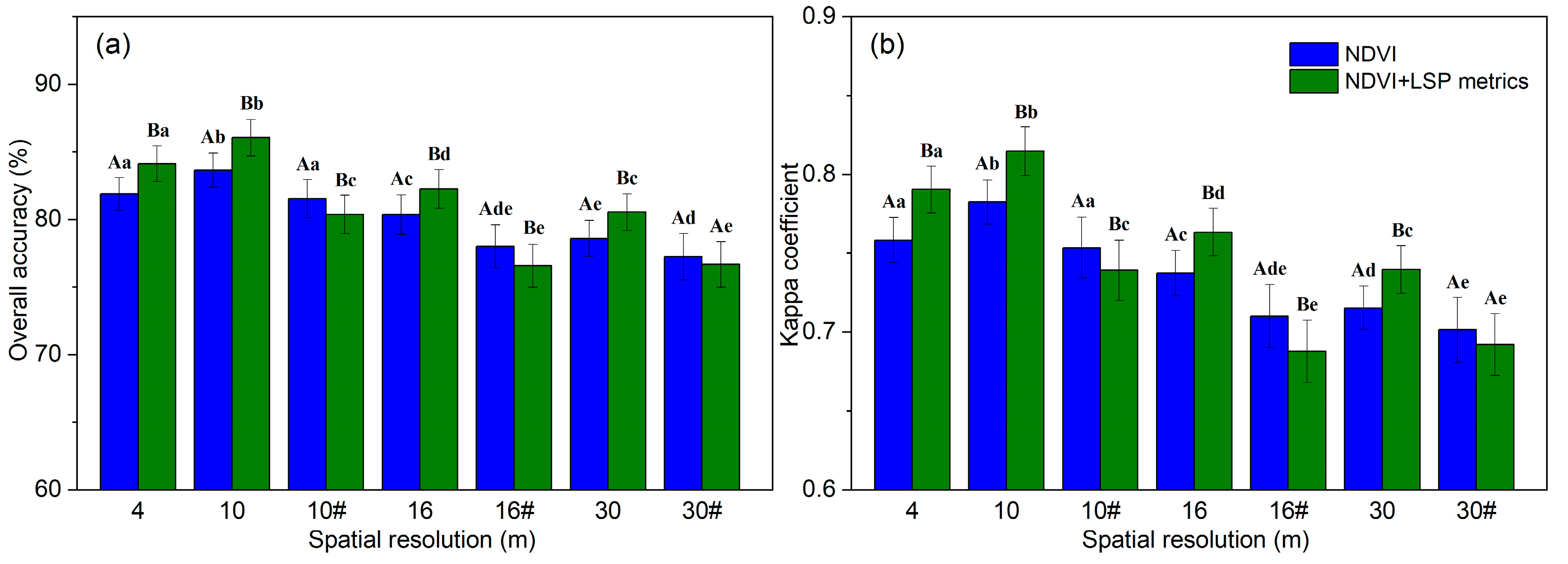
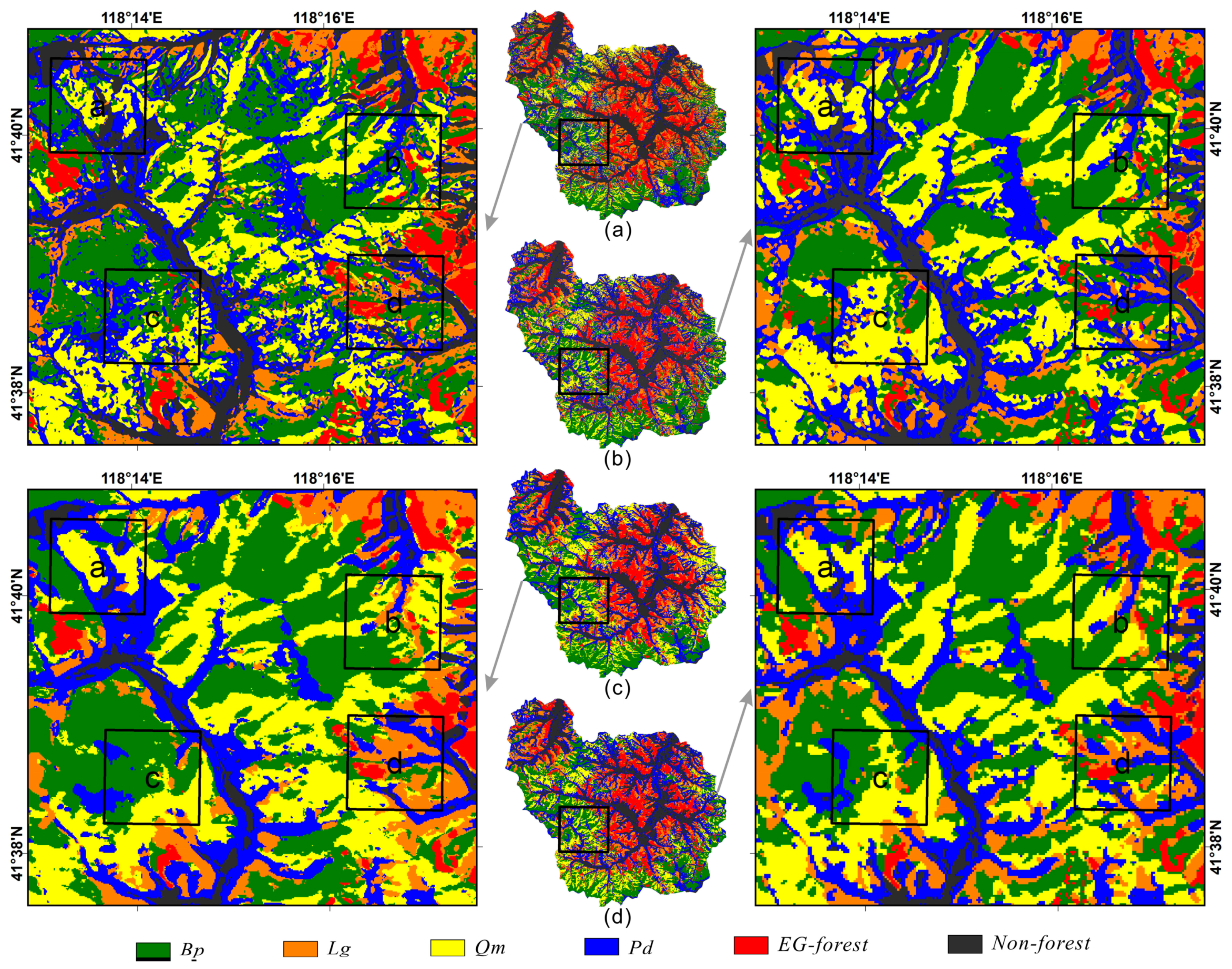
3.3. Multiscale Classification by Satellite Images and Up-Scaled Images

There were significant differences among the OA values of the dominant forest species at different spatial resolutions (p < 0.05; Figure 5a), while the Kappa values show consistent results (p < 0.05; Figure 5b). For multiscale satellite time-series NDVI images, the mean OA (Kappa) first increases while image resolution goes from 4 to 10 m (p < 0.05) at the highest accuracy of 83.63% (0.7825), and then decreases to the minimum accuracy of 78.60% (0.7154) at 30 m resolution (p < 0.05). The classification accuracies of forest tree species are closely related to the image resolutions, and an analysis of variance reveals significant differences between classification accuracies based on time-series satellite data of differing resolution (p < 0.05). Combining phenological metrics and time-series NDVI data can improve the mapping of the regional dominant tree species at each given resolution (p < 0.05; Figure 5). When the contrast is integrated with time-series NDVI and LSP metrics, the best overall accuracy (Kappa) of forested landscape identification with 10 m resolution increases to 86.05% (0.8147; p < 0.05).
However, for up-scaled time-series images, the classification accuracy of the dominant tree species decreases from 81.88% (0.7583) to 77.23% (0.7014) with the spatial resolution ranging from 4 to 30 m# (p < 0.05). Therefore, there is no significant difference appears between the classification accuracies of dominant tree species of up-scaled time-series data at the resolution of 16 and 30 m (p > 0.05). Finally, combining phenological metrics and time-series NDVI data does not increase the recognition accuracy but leads to the decline from 10 to 30 m# resolution, which differs obviously from the results of native multiscale satellite data at each same given resolution (p < 0.05).

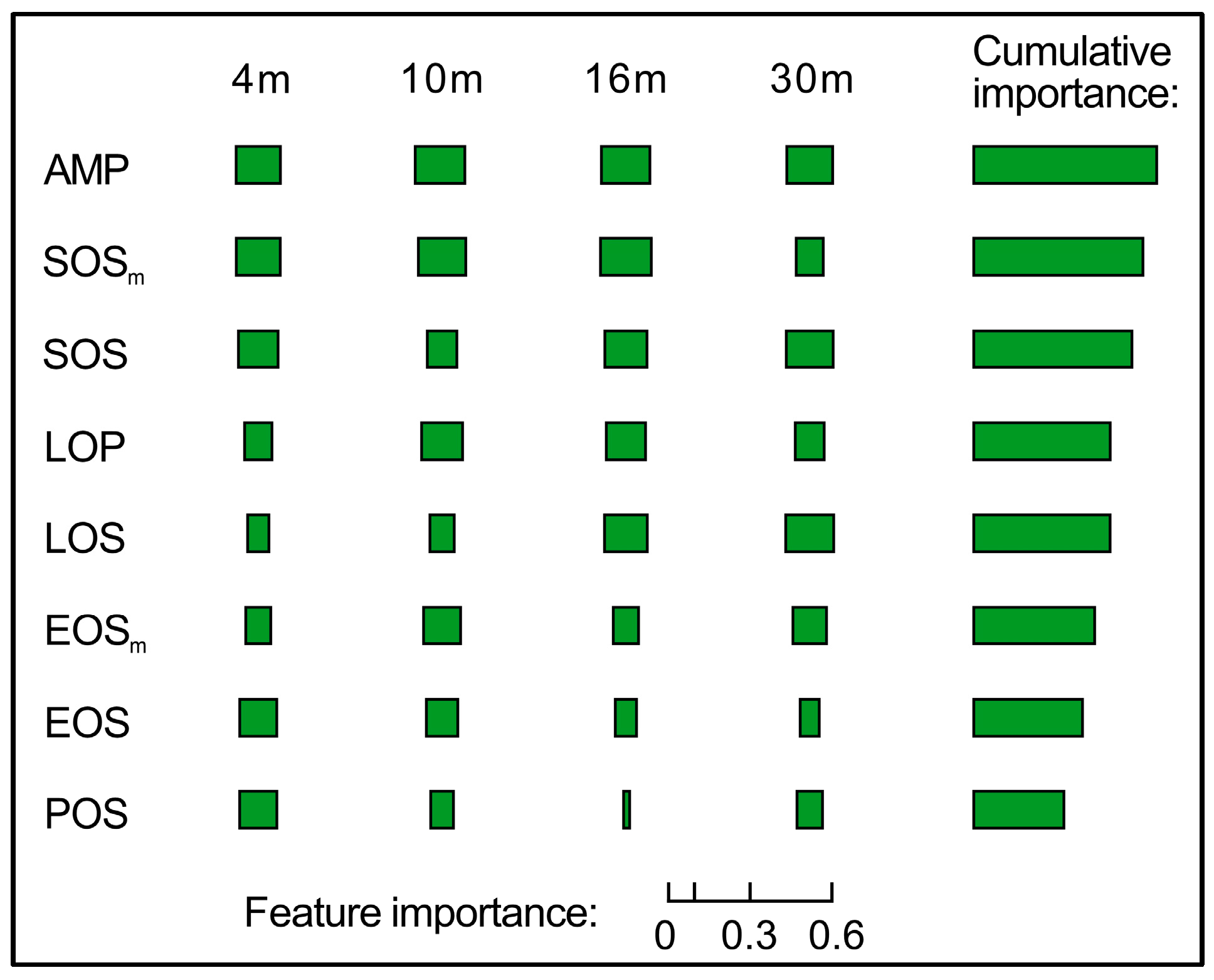
3.4. Contributions of Different LSP Metrics to Multiscale Tree Species Classification

The feature importance for identifying forest tree species using the eight LSP metrics of four image resolutions are different (Figure 6). Before analysis, each final feature importance for variables was averaged after ten cross-verifications. The results show that the LSP metrics are valuable for differentiating among forest tree species in the study region (p < 0.05). The various LSP metrics produce different positive effects on the classification of dominant tree species, although the magnitude of the influence varies (p < 0.05; Figure 6). When considering the four different spatial resolutions, the importance of each LSP metric turns out to be inhomogeneous (Figure 6). The phenological information such as SOSm, EOS, and POS are more important at higher image resolution, whereas only the LOS achieves the highest importance at lower spatial resolution. In addition, AMP and SOS show roughly the same degree of importance at different resolutions.
Testing the cumulative importance of each LSP metric for individual spatial resolutions reveals the importance of each variable from medium to high resolutions (Figure 6). At first, the LSP metrics in AMP, SOSm, and SOS are by far the three most important features (p < 0.05), showing the middle and early growth period account for the most important contribution in tree-species phenological observations. They are followed by LOP and LOS, which control the length of the growth period and the peak period. Subsequently, the remaining EOSm and EOS metrics represent the period of declining growth which has less importance. Finally, POS is the least important metric which indicates the peak time, and the differences of POS among the different dominant tree species are small.

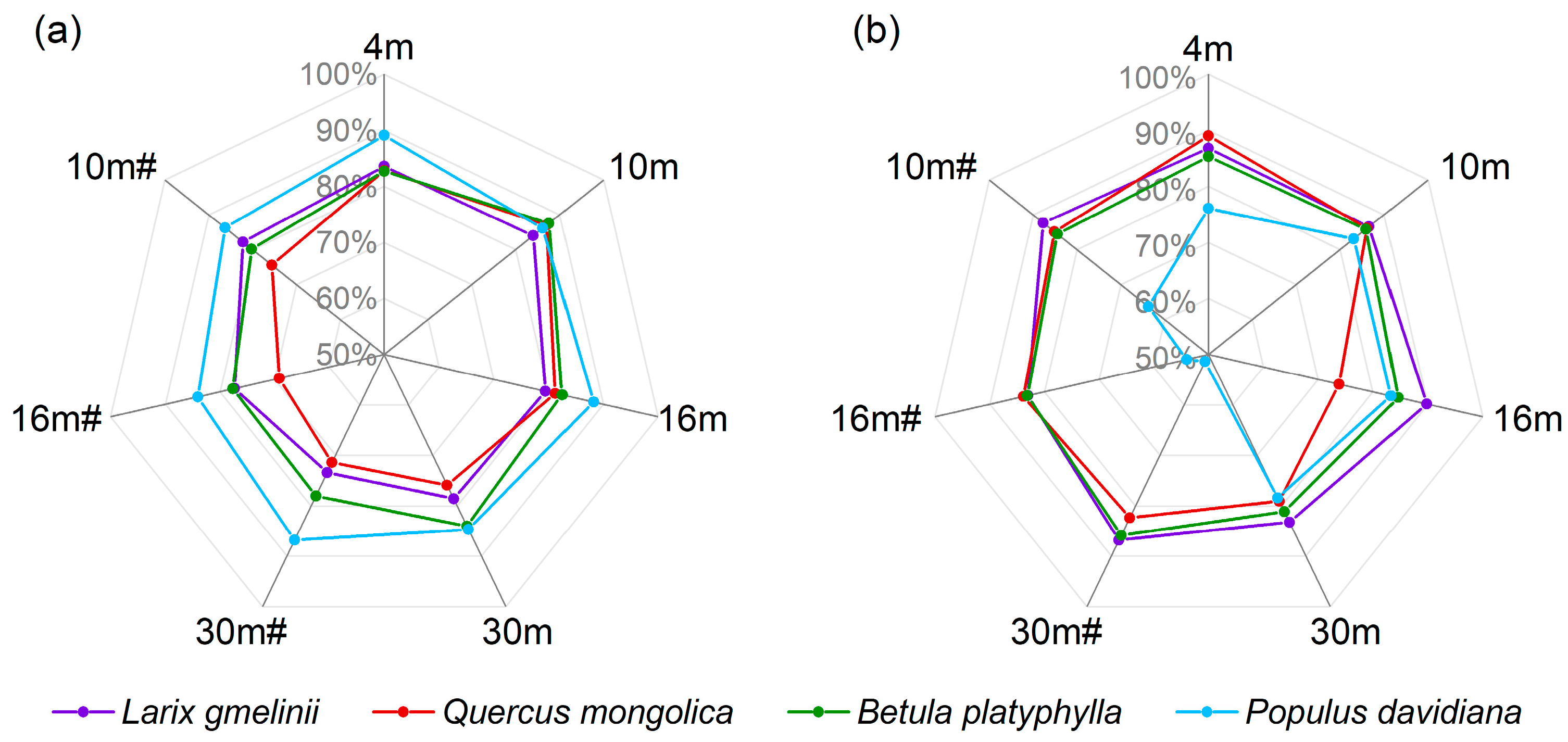
3.5. Comparisons of Accuracy for Producer and User of Dominant Tree Species

In native satellite images, the PA of Bp, Lg, Qm, Pd, and the UA of Bp, Lg, Qm show a downward trend on the whole with the decrease in spatial resolution goes from 4 to 30 m; except for the UA of Pd which increases at first and then decreases (Figure 7). None of the dominant classes of tree species have both a low UA and PA. The confusion matrix shows that many Bp, Lg, and Qm are misclassified into Pd in different spatial resolutions, which also leads to an over-mapping for Pd, so the UA of Pd is less than the PA from 4 to 30 m resolution, especially at 4 m. For the mapping results of forest tree species landscape (Figure 8), the comparison shows that the worst classification result occurs in imagery with 30 m resolution, where a portion of Qm and Lg is misclassified as Pd. In addition, some Lg are misclassified as Qm at 16 m resolution and the overall forest mapping at 10 m resolution is better than at 4 m resolution, which is mainly due to the higher mapping accuracy of Qm and Bp.
However, for up-scaled images, both PA and UA values of different deciduous species change only slightly when the spatial resolution goes down (Figure 7). The UA of Bp, Lg, and Qm and the PA of Pd change slightly from 4 to 30 m# resolution. At the same time, the UA of Bp, Lg, and Qm are significantly higher than their PA, except for Pd, implying over-mapping occurred. On the contrary, the forest tree species with high UA but low PA refer to under-mapping [77]. In this study, low PA of Bp, Lg, and Qm show that large areas of Bp, Lg, and Qm are not properly classified into their respective class, and their PA decrease as the image resolution goes down (Figure 7). In general, PA and UA of the most tree species for up-scaled data are often diminished and more unstable than that for real satellite data, furthermore, almost all tree species reaching their maximum value at the image resolution of 4 m.

4. Discussion

Spatial resolution significantly affects the identification of forest species and mapping based on single-date images [7,12,50,78]. Some studies have indicated that the NDVI temporal variation of stand canopy shows the detailed dynamics of timeline-based spectra of different forest types [14,15]. However, less attention has focused on the spatial scale of the uncertainty in the results. The present study confirms that the overall accuracy gradually extends from 78.59% to 83.63%, while the kappa synchronously increases from 0.7154 to 0.7825, which indicates that the classification accuracy of the dominant tree species is strongly linked to the spatial resolution of the time-series satellite data (p < 0.05). In this study, for a spatial resolution of 4 and 10 m, the classification accuracy is high (>81.88%), where the forest landscape identification is apparent, and each dominant species are classified correctly (p < 0.05). Overall, the time-series images with higher resolution (4–10 m) providing higher and more stable OA and kappa perform better in identifying the regional forest tree species than those with lower resolution (16–30 m). However, it does not mean that images with finer resolution can always provide more accurate results because it also depends on the selected feature datasets and classification methods.
The mean NDVI values of 4 m images are less than that of 10 m (p < 0.05; Figure 3), which we attribute to the NDVI being prematurely saturated at the higher resolution because a higher resolution correlates with less energy incident on the sensor, which decreases the spectral resolution [51,79]. Hence, the annual peak NDVI is mostly below 0.7 for the various dominant deciduous species at 4 m resolution, which is significantly less than the NDVI at the resolution of 10, 16, and 30 m, respectively (p < 0.05; Figure 3). Furthermore, the result is also assisted by the narrower near-infrared band and higher radiation resolution of Sentinel-2 image (12 bit, whereas 10 bit of the Gaofen-2 image), which could provide a better capability of vegetation information monitoring. It actually may overcome the negative effects of its coarser resolution to some extent. In addition, the multiscale annual mean NDVI of the sample data for different forest land remains essentially stable for up-scaled data (Figure 3). The spectral information in up-scaled images has a strong dependence on the input high-resolution images, which leads to discrepancies in comparison to actual imaging results at the given spatial resolution (Figure 3). As the image resolution decreases, the spectral information related to the forest tree species was smoothed which would increase omission and commission errors [80]. These results imply that the resampled time-series data have different spectral reflectance in comparison to native images acquired at the same resolution evidently (p < 0.05), which reduces the susceptibility to spatial resolution and barely represents the satellite image features of the same scale due to the spectral distortion [51]. Therefore, the classification results of tree species based on up-scaled images differ from those of native images for a given resolution (p < 0.05), indicating that native satellite data cannot be accurately replaced by up-scaled images.
Satellite remote sensing imagery is widely applied to monitor forest phenology on global and regional scales [42,43,44]. Plant phenology provides valuable information for classifying vegetation types [43], and some studies use spectral and phenological parameters to map crops [52,65,81]. However, research on mapping forest tree species has not considered the phenological metrics with images at a medium-high spatial resolution, which might introduce uncertainties in identifying and mapping different tree species [19]. Our classification results combined with NDVI and LSP metrics increases the OA (Kappa) by 2.24% (0.0322), 2.42% (0.0322), 1.89% (0.0258), and 1.94% (0.0243) at 4, 10, 16, and 30 m, respectively. For the 10 m time-series data, all deciduous tree species are correctly classified into their respective categories (Figure 8), and their UA and PA can reach more than 83.12%. These results show that using spatial resolution NDVI data combined with temporal phenological characteristics improves the accuracy of the results at each scale from 4 to 30 m (p < 0.05), which indicates that combining the spectral curve and the LSP metrics is a good way to identify and monitor the main forest ecosystem and may improve the precision of spatial mapping in temperate regions from medium to high spatial resolution.
Although differences appear in the phenological metrics at different resolutions, to some extent they have positive effects on the classification of forest tree species in this study region (Figure 6). The three highest phenological variables are AMP, SOSm, and SOS, based on the contribution of different phenological metrics and the classification of tree species. This indicates that the growth stage from germination to maximum growth and the amplitude of the growth spectrum contribute the most to the identification of the tree species. In addition, after combining the phenology metrics, the accuracy of the classification results based on the up-scaled data decreases by different degrees compared with the previous results (Figure 5). This is mainly contributed to the decrease in effective spectral information after the smoothing of up-scaled NDVI data and the increase in invalid band information, which would increase feature redundancy, leading to the further degradation of classification results [51,82].
Considering the special significance of phenology in spring [38,44,53], many previous studies were conducted to investigate the effects of forest spring phenology with different resolutions. However, most of them used up-scaled images due to a lack of multiresolution satellite data covering the area with a shorter revisit period [83]. Therefore, we investigate herein how scaling affects spring phenology (SOS) via a comparison between results from low- and high-resolution data. The results show that retrievals of SOS date reflect the difference in spatial scale, resulting in a delay as the resolution worsens. In this study, the SOS results of all species of Landsat-8 data (30 m) are earlier than that of Genfen-1 data (16 m). This result is mainly attributed to the better radiometric precision of Landsat-8 OLI (12 bit, whereas 10 bit of the Genfen-1) and the spectral range refinement of the near-infrared band (Table 1), which improves the overall signal to noise ratio for vegetation monitoring [51] and somewhat avoid overestimation [44] and further reasons need to be verified in follow-up studies. Relative to data with a medium-low resolution that is commonly used to monitor vegetation phenology, medium-high resolution satellites can achieve higher classification accuracy. This is because the observation of deciduous vegetation phenological characteristics is vulnerable to the interference of the evergreen forests or other background factors such as the stand age and topography [84,85]. As a consequence, medium-high resolution satellites can observe more spatial detail information and therefore capture the spectral variation of vegetation in phenology which is not normally detectable in data from sensors with lower spatial resolution.
However, the results show that estimations of spring phenology from up-scaled imagery have little noticeable change, corresponding less to the results derived from multiscale satellite remote sensing data. These findings are consistent with related studies based on up-scaled data. For example, Tian et al. (2021) resampled time-series images with 10 m to a series of lower spatial resolution images from 30 m to 8 km and obtained relatively stable vegetation SOS data in rural areas with a resolution ranging from 10 m to 8 km [53]. Similarly, another study found that the overall SOS averaged from images with a resolution ranging from 1 × 250 m to 35 × 250 m is generally similar but with a difference of fewer than five days [44]. Therefore, Zhang et al. (2017) suggested SOS datasets should be calculated from actual time-series images of different spatial scales but not the time-series data up-scaled from finer resolution imagery data using simple resampling methods [52].
In this study, both phenological monitoring and the classification of forest tree species differ significantly when using multiscale satellite images and up-scaled images because of the differences in the imaging mechanism. Related research revealed the difference between the native satellite data and up-scaled data is determined by the mechanism of remote sensing imaging, in which the most up-scaled results are spatial insensitive because of not considering the spatial adjacent information of landscapes [51,86], nor adjusting as the variation of spectral reflection properties at different spatial resolutions [87]. Therefore, the up-scaled images cannot be directly used to replace remote sensing images in time-series monitoring or quantitative analysis. Therefore, methods are gradually being developed to scale-transformation model involving physical mechanism [86,87,88,89] and temporal–spatial fusion algorithms [23,53,90], to ensure image features from different spatial resolutions can be integrated into applications.
This study expands on previous work in two important ways: First, we continue to compare tree species classification for multiscale time-series images and explore the applicability of remote sensing images to the study of LSP metrics. Next, we discuss how spatial-scale uncertainty affects phenological observations and the classification of dominant tree species. In addition, we try to construct herein monthly time-series multiscale satellite images with resolutions ranging from 4 to 30 m. In fact, the monthly time-series data has proven to suffice to describe the one-year spectral curve dynamics of forest tree species when cloud-free imagery is available at specific phenological stages [17,24,70]. However, some studies have shown that more intensive time-series images would be better at capturing fine dynamic differences to separate information on similar forest tree species [19,91]. With recent breakthroughs in multispectral remote-sensing, the temporal-spatial resolution of satellite data is improved obviously. Using imagery from more advanced sensors will enhance the precision of forest phenology monitoring and tree species classification. Therefore, more intensive time-series multiscale images are required to extend the results in this paper.

5. Conclusions

The spatial resolution of satellite remote sensing data has a major impact on forest information extraction and dynamic monitoring, and it is critical to the success of regional dominant tree species mapping. This study develops a process for reconstructing time-series satellite images with medium-high spatial resolution and applies it to monitor forest phenology and map tree species. The study also examines how time-series spectral data responds to the scaling effect obtained from various spatial resolution satellites. Moreover, we discuss how spatial resolution and LSP metrics affect the classification of dominant tree species. The results indicate that remote sensing images with 10 m resolution are more appropriate for the time-series-based forest tree-species classification with superior performance in the study region. In addition, the use of additional LSP metrics further improves the classification results, so they are highly recommended.
Nowadays, though the temporal resolution of remote sensing data is improving, few pieces of research have been designed to investigate how up-scaled time-series images affect forest mapping on landscapes. The present results elaborate the general pattern of time-series remote-sensing tree species identification and spring phenology extraction with medium-high spatial resolution. Therefore, a significant difference was found by contrasting the forest landscape classification results obtained from real multiscale time-series satellite data with that of up-scaled time-series images. This work thus provides a primary understanding of how to use and compare time-series remote sensing images with different spatial resolutions for forest monitoring.

Author Contributions

Conceptualization and Methodology, K.X.; Software and Data Curation, Z.Z. and W.Y.; Formal analysis, J.Y. and W.Y.; Validation, P.Z. and Y.D.; Writing—Original Draft, K.X.; Writing—Review and Editing, Z.Z. and J.Y.; Data collection and processing K.X. and J.G. All authors have read and agreed to the published version of the manuscript.

Funding

This research was funded by the Anhui Provincial Natural Science Foundation of China, grant number 2008085QD193, and the Fundamental Research Funds for the Central Universities of China, grant number JZ2020HGQA0189 and JZ2021HGTA0166.

Data Availability Statement

The data that we used in this study can be requested by contacting the corresponding author.

Acknowledgments

The authors thank Shengnan Jiang for her assistance with the revision of the manuscript.

Conflicts of Interest

The authors declare no conflict of interest.

Appendix A

Table A1. The information of satellite images used in this study.
MonthImaging Date (Gaofen-2)Imaging Date (Sentinel-2)Imaging Date (Gaofen-1)Imaging Date (Landsat-8)
January20180121201801202018011720180111
February20180215201802142018021420180212
March20180316201803112018031120180316
April20180430201804152018041820180417
May20180510201805152018051520180519
June20180608201806142018062120180620
July20180722201807292018072220180706
August20180816201808232018082020180823
September20170920201709222018091620180924
October20181019201810172018101920181025
November20181118201811212018112020181126
December20181213201812162018121520181213
Table A2. Characteristics of the dominant tree species in this study.
Species NamePictureMain Characteristics
Larix gmelinii (Lg) Remotesensing 13 02716 i001
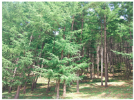
A deciduous tree (30 m), D.B.H. 90 cm or so. The barks are taupe, and the branches consist of obvious long branches and short branches. Light-loving, cold-resistant, drought-resistant. Mainly distributed in Northeast China as well as the mountainous areas from eastern Inner Mongolia to eastern Siberia of Russia.
Populus davidiana (Pd) Remotesensing 13 02716 i002
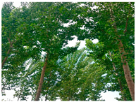
A deciduous tree (25 m), D.B.H. 60 cm or so. The barks are gray or gray-green, and the leaves are ovate or nearly round with incised margin. Light-loving, cold-resistant, and soil are adaptable. Mainly distributed in valleys of high mountains in Northeast China, Northwest China, North China and Southwest China.
Betula platyphylla (Bp) Remotesensing 13 02716 i003
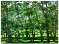
A deciduous tree (27 m), D.B.H. 80 cm or so. The barks are white and smooth or local cracking, and the leaves are ovate with a jagged margin. Light-loving, cold-loving, and soil adaptable. Mainly distributed in Northeast China, North China and the mountainous areas on the outer edge of the Qinghai-Tibet Plateau.
Quercus mongolica (Qm) Remotesensing 13 02716 i004
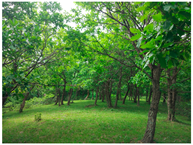
A deciduous tree (30 m), D.B.H. 60 cm or so. The barks are dark taupe, the branches are purplish-brown, the leaves are obovate with around margin. Light-loving, soil adaptable. Mainly distributed in Northeast China and part of northern North China.

References

  1. Sannier, C.; McRoberts, R.E.; Fichet, L. Suitability of global forest change data to report forest cover estimates at national level in Gabon. Remote Sens. Environ. 2016, 173, 326–338. [Google Scholar] [CrossRef]
  2. Feng, Y.; Lu, D.S.; Chen, Q.; Keller, M.; Moran, E.; Dos-Santo, M.N.; Bolf, E.L.; Batistella, M. Examining effective use of data sources and modeling algorithms for improving biomass estimation in a moist tropical forest of the Brazilian Amazon. Int. J. Digit. Earth 2017, 10, 996–1016. [Google Scholar] [CrossRef]
  3. Frenne, P.D.; Zellweger, F.; Rodríguez-Sánchez, F.; Scheffers, B.R.; Hylander, K.; Luoto, M.; Vellend, M.; Verheyen, K.; Lenoir, J. Global buffering of temperatures under forest canopies. Nat. Ecol. Evol. 2019, 3, 744–749. [Google Scholar] [CrossRef] [PubMed]
  4. Heinzel, J.; Koch, B. Investigating multiple data sources for tree species classification in temperate forest and use for single tree delineation. Int. J. Appl. Earth Obs. 2012, 18, 101–110. [Google Scholar] [CrossRef]
  5. Fassnacht, F.E.; Latifi, H.; Stereńczak, K.; Modzelewska, A.; Lefsky, M.; Waser, L.T.; Straub, C.; Ghosh, A. Review of studies on tree species classification from remotely sensed data. Remote Sens. Environ. 2016, 186, 64–87. [Google Scholar] [CrossRef]
  6. Meddens, A.H.; Hicke, J.A.; Vierling, L.A. Evaluating the potential of multispectral imagery to map multiple stages of tree mortality. Remote Sens. 2011, 115, 1632–1642. [Google Scholar] [CrossRef]
  7. Ghosh, A.; Fassnacht, F.E.; Joshi, P.K.; Koch, B. A framework for mapping tree species combining hyperspectral and LiDAR data: Role of selected classifiers and sensor across three spatial scales. Int. J. Appl. Earth Obs. Geoinf. 2014, 26, 49–63. [Google Scholar] [CrossRef]
  8. Tang, L.N.; Shao, G.F. Drone remote sensing for forestry research and practices. J. For. Res. 2015, 26, 791–797. [Google Scholar] [CrossRef]
  9. Immitzer, M.; Böck, S.; Einzmann, K.; Vuolo, F.; Pinnel, N.; Wallner, A.; Atzberger, C. Fractional cover mapping of spruce and pine at 1 ha resolution combining very high and medium spatial resolution satellite imagery. Remote Sens. Environ. 2017, 204, 690–703. [Google Scholar] [CrossRef] [Green Version]
  10. Wu, H.; Li, Z.L. Scale issues in remote sensing: A review on analysis, processing and modeling. Sensors 2009, 9, 1768–1793. [Google Scholar] [CrossRef] [PubMed]
  11. Zhu, X.L.; Liu, D.S. Accurate mapping of forest types using dense seasonal Landsat time-series. ISPRS J. Photogramm. Remote Sens. 2014, 96, 1–11. [Google Scholar] [CrossRef]
  12. Roth, K.l; Roberts, D.A.; Dennison, P.E.; Peterson, S.H.; Alonzo, M. The impact of spatial resolution on the classification of plant species and functional types within imaging spectrometer data. Remote Sens. Environ. 2015, 171, 45–57. [Google Scholar] [CrossRef]
  13. Pu, R.; Landry, S.; Yu, Q. Assessing the potential of multi-seasonal high resolution Pléiades satellite imagery for mapping urban tree species. Int. J. Appl. Earth Obs. Geoinf. 2018, 71, 144–158. [Google Scholar] [CrossRef]
  14. Dudley, K.L.; Dennison, P.E.; Roth, K.L.; Roberts, D.A.; Coates, A.R. A multi-temporal spectral library approach for mapping vegetation species across spatial and temporal phenological gradients. Remote Sens. Environ. 2015, 167, 121–134. [Google Scholar] [CrossRef]
  15. Grabska, E.; Hostert, P.; Pflugmacher, D.; Ostapowicz, K. Forest stand species mapping using the Sentinel-2 time series. Remote Sens. 2019, 11, 1197. [Google Scholar] [CrossRef] [Green Version]
  16. Kempeneers, P.; Sedano, F.; Seebach, L.M.; Strobl, P.; San-Miguel-Ayanz, J. Data fusion of different spatial resolution remote sensing images applied to forest-type mapping. IEEE T. Geocsi. Remote. 2011, 49, 4977–4986. [Google Scholar] [CrossRef]
  17. Atkinson, P.M.; Jeganathan, C.; Dash, J.; Atzberger, C. Inter-comparison of four models for smoothing satellite sensor time-series data to estimate vegetation phenology. Remote Sens. Environ. 2012, 123, 400–417. [Google Scholar] [CrossRef]
  18. Granero-Belinchon, C.; Adeline, K.; Briottet, X. Impact of the number of dates and their sampling on a NDVI time series reconstruction methodology to monitor urban trees with Venμs satellite. Int. J. Appl. Earth Obs. Geoinf. 2021, 95, 102257. [Google Scholar] [CrossRef]
  19. Xu, K.J.; Tian, Q.J.; Zhang, Z.Y.; Yue, J.B.; Chang, C.T. Tree species (genera) identification with GF-1 time-series in a forested landscape, Northeast China. Remote Sens. 2020, 12, 1554. [Google Scholar] [CrossRef]
  20. Kollert, A.; Bremer, M.; Löw, M.; Rutzinger, M. Exploring the potential of land surface phenology and seasonal cloud free composites of one year of Sentinel-2 imagery for tree species mapping in a mountainous region. Int. J. Appl. Earth Obs. 2021, 94, 102208. [Google Scholar] [CrossRef]
  21. Li, X.; Chen, W.Y.; Sanesi, G.; Lafortezza, R. Remote sensing in urban forestry: Recent applications and future directions. Remote Sens. 2019, 11, 1144. [Google Scholar] [CrossRef] [Green Version]
  22. Hill, R.A.; Wilson, A.K.; George, M.; Hinsley, S.A. Mapping tree species in temperate deciduous woodland using time-series multi-spectral data. Appl. Veg. Sci. 2010, 13, 86–99. [Google Scholar] [CrossRef]
  23. Jia, K.; Liang, S.; Wei, X.; Yao, Y.; Su, Y.; Jiang, B.; Wang, X. Land cover classification of Landsat data with phenological features extracted from time series MODIS NDVI data. Remote Sens. 2014, 6, 11518–11532. [Google Scholar] [CrossRef] [Green Version]
  24. Masemola, C.; Cho, M.A.; Ramoelo, A. Sentinel-2 time series based optimal features and time window for mapping invasive Australian native Acacia species in KwaZulu Natal, South Africa. Int. J. Appl. Earth Obs. Geoinf. 2020, 93, 102207. [Google Scholar] [CrossRef]
  25. Gessner, U.; Machwitz, M.; Conrad, C.; Dechab, S. Estimating the fractional cover of growth forms and bare surface in savannas. A multi-resolution approach based on regression tree ensembles. Remote Sens. Environ. 2013, 129, 90–102. [Google Scholar] [CrossRef] [Green Version]
  26. Achard, F.; Estreguil, C. Forest classification of Southeast Asia using NOAA AVHRR data. Remote Sens. Environ. 1995, 54, 198–208. [Google Scholar] [CrossRef]
  27. Xiao, X.M.; Boles, S.; Liu, J.Y.; Zhuang, D.F.; Liu, M.L. Characterization of forest types in Northeastern China, using multi-temporal SPOT-4 VEGETATION sensor data. Remote Sens. Environ. 2002, 82, 335–348. [Google Scholar] [CrossRef]
  28. Yu, X.F.; Zhuang, D.F.; Chen, H.; Hou, X.Y. Forest classification based on MODIS time series and vegetation phenology. In Proceedings of the IEEE International Geoscience and Remote Sensing Symposium, Anchorage, AK, USA, 20–24 September 2004; Volume 4, pp. 2369–2372. [Google Scholar] [CrossRef]
  29. Pimple, U.; Sitthi, A.; Simonetti, D.; Pungkul, S.; Leadprathom, K.; Chidthaisong, A. Topographic correction of Landsat TM-5 and Landsat OLI-8 imagery to improve the performance of forest classification in the mountainous terrain of Northeast Thailand. Sustainability 2017, 9, 258. [Google Scholar] [CrossRef] [Green Version]
  30. Yin, H.; Khamzina, A.; Pflugmacher, D.; Martius, C. Forest cover mapping in post-Soviet Central Asia using multi-resolution remote sensing imagery. Sci. Rep. 2017, 7, 1–11. [Google Scholar] [CrossRef] [Green Version]
  31. Townshend, J.R.; Masek, J.G.; Huang, C.; Vermote, E.F.; Gao, F.; Channan, S.; Sexton, J.O.; Feng, M.; Narasimhan, R.; Kim, D.; et al. Global characterization and monitoring of forest cover using Landsat data: Opportunities and challenges. Int. J. Digit. Earth 2012, 5, 373–397. [Google Scholar] [CrossRef] [Green Version]
  32. Ota, T.; Mizoue, N.; Yoshida, S. Influence of using texture information in remote sensed data on the accuracy of forest type classification at different levels of spatial resolution. J. For. Res. 2011, 16, 432–437. [Google Scholar] [CrossRef]
  33. Pu, R.L.; Bell, S. Mapping seagrass coverage and spatial patterns with high spatial resolution IKONOS imagery. Int. J. Appl. Earth Obs. Geoinf. 2017, 54, 145–158. [Google Scholar] [CrossRef]
  34. Puzzolo, V.; Denatale, F.; Gianne, F. Forest species discrimination in an Alpine mountain area using a fuzzy classification of multi-temporal SPOT (HRV) data. IEEE Int. Geosci. Remote Sens. Symp. 2003, 4, 2538–2540. [Google Scholar] [CrossRef]
  35. Persson, M.; Lindberg, E.; Reese, H. Tree species classification with multi-temporal Sentinel-2 data. Remote Sens. 2018, 10, 1794. [Google Scholar] [CrossRef] [Green Version]
  36. Wessel, M.; Brandmeier, M.; Tiede, D. Evaluation of different machine learning algorithms for scalable classification of tree types and tree species based on Sentinel-2 data. Remote Sens. 2018, 10, 1419. [Google Scholar] [CrossRef] [Green Version]
  37. Gomez, C.; White, J.C.; Wulder, M.A. Optical remotely sensed time series data for land cover classification: A review. ISPRS J. Photogramm. Remote Sens. 2016, 116, 55–72. [Google Scholar] [CrossRef] [Green Version]
  38. Liu, J.H.; Pan, Y.Z.; Zhu, X.F.; Zhu, W.Q. Using phenological metrics and the multiple classifier fusion method to map land cover types. J. Appl. Remote Sens. 2014, 8, 083691. [Google Scholar] [CrossRef]
  39. Michez, A.; Piegay, H.; Jonathan, L.; Claessens, H.; Lejeune, P. Mapping of riparian invasive species with supervised classification of Unmanned Aerial System (UAS) imagery. Int. J. Appl. Earth Obs. 2015, 44, 88–94. [Google Scholar] [CrossRef]
  40. Xu, K.J.; Tian, Q.J.; Xu, N.X.; Yue, J.B.; Tang, S.F. Classifying forest dominant trees species based on high dimensional time-series NDVI data and differential transform methods. Spectrosc. Spectr. Anal. 2019, 39, 3794–3800. [Google Scholar] [CrossRef]
  41. Kong, J.X.; Zhang, Z.C.; Zhang, J. Classification and identification of plant species based on multi-source remote sensing data: Research progress and prospect. Biodivers. Sci. 2019, 27, 796–812. [Google Scholar] [CrossRef]
  42. Peng, D.; Wu, C.; Zhang, X.; Yu, L.; Huete, A.R.; Wang, F.; Luo, S.; Liu, X.; Zhang, H. Scaling up spring phenology derived from remote sensing images. Agric. For. Meteorol. 2018, 256–257, 207–219. [Google Scholar] [CrossRef]
  43. Zeng, L.L.; Wardlow, B.D.; Xiang, D.X.; Hu, S.; Li, D. A review of vegetation phenological metrics extraction using time-series, multispectral satellite data. Remote Sens. Environ. 2020, 237, 111511. [Google Scholar] [CrossRef]
  44. Peng, D.; Zhang, X.; Zhang, B.; Liu, L.; Liu, X.; Huete, A.R.; Huang, W.; Wang, S.; Luo, S.; Zhang, X.; et al. Scaling effects on spring phenology detections from MODIS data at multiple spatial resolutions over the contiguous United States. ISPRS J. Photogramm. Remote Sens. 2017, 132, 185–198. [Google Scholar] [CrossRef]
  45. Ge, Q.; Dai, J.; Cui, H.; Wang, H. Spatiotemporal variability in start and end of growing season in China related to climate variability. Remote Sens. 2016, 8, 433. [Google Scholar] [CrossRef] [Green Version]
  46. Liu, L.; Cao, R.; Shen, M.; Chen, J.; Zhang, X. How does scale effect influence spring vegetation phenology estimated from satellite-derived vegetation indexes? Remote Sens. 2019, 11, 2137. [Google Scholar] [CrossRef] [Green Version]
  47. Liu, W.J.; Zeng, Y.N.; Zhang, M. Mapping rice paddy distribution by using time series HJ blend data and phenological parameters. J. Remote Sens. 2018, 22, 381–391. [Google Scholar] [CrossRef]
  48. Schwieder, M.; Leitão, P.J.; Pinto, J.R.; Teixeira, A.C.; Pedroni, F.; Sanchez, M.; Bustamante, M.M.; Hostert, P. Landsat phenological metrics and their relation to aboveground carbon in the Brazilian Savanna. Carbon Balanc. Manag. 2018, 13, 1–15. [Google Scholar] [CrossRef] [Green Version]
  49. Schaaf, A.; Dennison, P.; Fryer, G.; Roth, K.; Roberts, D. Mapping plant functional types at multiple spatial resolutions using imaging spectrometer data. GISci. Remote Sens. 2011, 48, 324–344. [Google Scholar] [CrossRef]
  50. Peña, M.A.; Cruz, P.; Roig, M. The effect of spectral and spatial degradation of hyperspectral imagery for the sclerophyll tree species classification. Int. J. Remote Sens. 2013, 34, 7113–7130. [Google Scholar] [CrossRef]
  51. Xu, K.J.; Tian, Q.J.; Yang, Y.J.; Yue, J.B.; Tang, S.F. How up-scaling of remote-sensing images affects land-cover classification by comparison with multiscale satellite images. Int. J. Remote Sens. 2019, 40, 2784–2810. [Google Scholar] [CrossRef]
  52. Zhang, X.; Wang, J.; Gao, F.; Liu, Y.; Schaaf, C.; Friedl, M.; Yu, Y.; Jayavelu, S.; Gray, J.; Liu, L.; et al. Exploration of scaling effects on coarse resolution land surface phenology. Remote Sens. Environ. 2017, 190, 318–330. [Google Scholar] [CrossRef] [Green Version]
  53. Tian, J.Q.; Zhu, X.L.; Wu, J.; Shen, M.G.; Chen, J. Coarse-resolution satellite images overestimate urbanization effects on vegetation spring phenology. Remote Sens. 2020, 12, 117. [Google Scholar] [CrossRef] [Green Version]
  54. Moody, A.; Woodcock, C.E. Scale-dependent errors in the estimation of land-cover proportions: Implications for global land-cover datasets. Photogramm. Eng. Remote Sens. 1994, 60, 585–594. [Google Scholar]
  55. Luan, H.J.; Tian, Q.J.; Yu, T.; Hu, X.L.; Huang, Y.; Liu, L.; Du, L.T.; Wei, X. Review of up-scaling of quantitative remote sensing. Adv. Earth Sci. 2013, 28, 657–664. [Google Scholar] [CrossRef]
  56. Chen, J.; Jönsson, P.; Tamura, M.; Gu, Z.; Matsushita, B.; Eklundh, L. A simple method for reconstructing a high-quality NDVI time-series data set based on the Savitzky-Golay filter. Remote Sens. Environ. 2004, 91, 332–344. [Google Scholar] [CrossRef]
  57. Wang, Y.F.; Xue, Z.H.; Chen, J.; Chen, G.Z. Spatio-temporal analysis of phenology in Yangtze river delta based on MODIS NDVI time series from 2001 to 2015. Front. Earth Sci. 2019, 13, 92–110. [Google Scholar] [CrossRef]
  58. Shao, Y.; Lunetta, R.S.; Wheeler, B.; Iiames, J.S.; Campbell, J.B. An evaluation of time-series smoothing algorithms for land-cover classifications using MODIS-NDVI multi-temporal data. Remote Sens. Environ. 2016, 174, 258–265. [Google Scholar] [CrossRef]
  59. Xu, K.J.; Zeng, H.D.; Zhu, X.B.; Tian, Q.J. Evaluation of five commonly used atmospheric correction algorithms for multi-temporal aboveground forest carbon storage estimation. Spectrosc. Spect. Anal. 2017, 37, 3493–3498. [Google Scholar] [CrossRef]
  60. Jönnson, P.; Eklundh, L. TIMESAT-a program for analyzing time-series of satellite sensor data. Comput. Geosci. 2004, 30, 833–845. [Google Scholar] [CrossRef] [Green Version]
  61. Chang, C.T.; Wang, H.C.; Huang, C. Impact of vegetation onset time on the net primary productivity in a mountainous island in Pacific Asia. Environ. Res. Lett. 2013, 8, 05030. [Google Scholar] [CrossRef] [Green Version]
  62. Yang, Y.T.; Guan, H.D.; Shen, M.G.; Liang, W.; Jiang, L. Changes in autumn vegetation dormancy onset date and the climate controls across temperate ecosystems in China from 1982 to 2010. Glob. Chang. Biol. 2014, 21, 1–14. [Google Scholar] [CrossRef]
  63. Heumann, B.W.; Seaquist, J.W.; Eklundh, L.; Jönsson, P. AVHRR derived phenological change in the Sahel and Soudan, Africa, 1982-2005. Remote Sens. Environ. 2007, 108, 385–392. [Google Scholar] [CrossRef]
  64. Jiao, F.S.; Liu, H.Y.; Xu, X.J.; Gong, H.B.; Lin, Z.S. Trend evolution of vegetation phenology in China during the period of 1981–2016. Remote Sens. 2020, 12, 572. [Google Scholar] [CrossRef] [Green Version]
  65. Lebrini, Y.; Boudhar, A.; Hadria, R.; Lionboui, H.; Elmansouri, L.; Arrach, R.; Ceccato, P.; Benabdelouahab, T. Identifying agricultural systems using SVM classification approach based on phenological metrics in a semi-arid region of Morocco. Earth Syst. Environ. 2019, 3, 277–288. [Google Scholar] [CrossRef]
  66. Sothe, C.; de Almeida, C.M.; Liesenberg, V.; Schimalski, M.B. Evaluating Sentinel-2 and Landsat-8 data to map sucessional forest stages in a subtropical forest in southern Brazil. Remote Sens. 2017, 9, 838. [Google Scholar] [CrossRef] [Green Version]
  67. Breiman, L. Random forests. Mach. Learn. 2001, 45, 5–32. [Google Scholar] [CrossRef] [Green Version]
  68. Immitzer, M.; Vuolo, F.; Atzberger, C. First experience with Sentinel-2 data for crop and tree species classifications in central Europe. Remote Sens. 2016, 8, 166. [Google Scholar] [CrossRef]
  69. Belgiu, M.; Drăgut, L. Random forest in remote sensing: A review of applications and future directions. ISPRS J. Photogramm. Remote Sens. 2016, 114, 24–31. [Google Scholar] [CrossRef]
  70. Immitzer, M.; Atzberger, C.; Koukal, T. Tree species classification with random forest using very high spatial resolution 8-band WorldView-2 satellite data. Remote Sens. 2012, 4, 2661–2693. [Google Scholar] [CrossRef] [Green Version]
  71. Reyes-Palomeque, G.; Dupuy, J.M.; Portillo-Quintero, C.A.; Andrade, J.L.; Tun-Dzul, F.J.; Hernández-Stefanoni, J.L. Mapping forest age and characterizing vegetation structure and species composition in tropical dry forests. Ecol. Indic. 2021, 120, 106955. [Google Scholar] [CrossRef]
  72. Chutia, D.; Bhattacharyya, D.K.; Sarma, K.K.; Kalita, R.; Sudhakar, S. Hyperspectral remote sensing classifications: A perspective survey. Trans. GIS 2016, 20, 463–490. [Google Scholar] [CrossRef]
  73. Shang, X.; Chisholm, L. Classification of Australian native forest species using hyperspectral remote sensing and machine-learning classification algorithms. IEEE J. Sel. Top. Appl. Earth Obs. Remote Sens. 2014, 7, 2481–2489. [Google Scholar] [CrossRef]
  74. Han, H.; Lee, S.; Im, J.; Kim, M.; Lee, M.I.; Ahn, M.; Chung, S.R. Detection of convective initiation using meteorological imager onboard communication, ocean, and meteorological satellite based on machine learning approaches. Remote Sens. 2015, 7, 9184–9204. [Google Scholar] [CrossRef] [Green Version]
  75. Immitzer, M.; Neuwirth, M.; Bck, S.; Brenner, H.; Atzberger, C. Optimal input features for tree epecies classification in central Europe based on multi-temporal Sentinel-2 data. Remote Sens. 2019, 11, 2599. [Google Scholar] [CrossRef] [Green Version]
  76. Janssen, L.L.F.; van der Wel, F.J.M. Accuracy assessment of satellite derived land-gover data: A review. Photogramm. Eng. Remote Sens. 1994, 60, 419–426. [Google Scholar] [CrossRef]
  77. Yang, Y.; Xiao, P.; Feng, X.; Li, H. Accuracy assessment of seven global land cover datasets over China. ISPRS J. Photogramm. Remote Sens. 2017, 125, 156–173. [Google Scholar] [CrossRef]
  78. Richter, R.; Reu, B.; Wirth, C.; Doktor, D.; Vohland, M. The use of airborne hyperspectral data for tree species classification in a species-rich Central European forest area. Int. J. Appl. Earth Obs. Geoinf. 2016, 52, 464–474. [Google Scholar] [CrossRef]
  79. Wang, L.; Yang, R.; Tian, Q.; Yang, Y.; Zhou, Y.; Sun, Y.; Mi, X. Comparative analysis of GF-1 WFV, ZY-3 MUX, and HJ-1 CCD sensor data for grassland monitoring applications. Remote Sens. 2015, 7, 2089–2108. [Google Scholar] [CrossRef] [Green Version]
  80. Li, N.; Xie, G.D.; Zhou, D.M.; Zhang, C.S.; Jiao, C.C. Remote sensing classification of marsh wetland with different resolution images. J. Resour. Ecol. 2016, 7, 107–114. [Google Scholar] [CrossRef]
  81. Lessel, J.; Ceccato, P. Creating a basic customizable framework for crop detection using Landsat imagery. Int J. Remote Sens. 2016, 37, 6097–6107. [Google Scholar] [CrossRef]
  82. Hu, Y.F.; Xu, Z.Y.; Liu, Y.; Yan, Y.; Wang, Q.Q. Accuracy analysis of up-scaling data: A case study with land use data in Xilin Gol of Inner Mongolia, China. Geogr. Res. 2012, 31, 1961–1972. [Google Scholar] [CrossRef]
  83. Zhang, Z.; Tao, Y.U.; Meng, Q.; Xinli, H.U.; Chang, L.I. Image Quality Evaluation of Multi-Scale Resampling in Geometric Correction. J. Huazhong Norm. Univ. 2013, 47, 426–430. [Google Scholar] [CrossRef]
  84. Melaas, E.K.; Friedl, M.A.; Zhu, Z. Detecting interannual variation in deciduous broadleaf forest phenology using Landsat TM/ETM+ data. Remote Sens. Environ. 2013, 132, 176–185. [Google Scholar] [CrossRef]
  85. Tang, S.F.; Tian, Q.J.; Xu, K.J.; Xu, N.X.; Yue, J.B. Age information retrieval of Larix gmelinii forest using Sentinel-2 data. J. Remote Sens. 2020, 24, 1511–1524. [Google Scholar] [CrossRef]
  86. Hay, G.J.; Niernann, K.O.; Goodenough, D.J. Spatial thresholds, image-objects, and upscaling: A multiscale evaluation. Remote Sens. Environ. 1997, 62, 1–19. [Google Scholar] [CrossRef]
  87. Tian, Y.; Wang, Y.; Zhang, Y.; Knyazikhin, Y.; Bogaert, J.; Mynemi, R.B. Radiative transfer based scaling of LAI retrieval from reflectance data of different resolutions. Remote Sens. Environ. 2002, 84, 143–159. [Google Scholar] [CrossRef]
  88. Wu, H.; Tang, B.H.; Li, Z.L. Impact of nonlinearity and discontinuity on the spatial scaling effects of the leaf area index retrieved from remotely sensed data. Int. J. Remote Sens. 2013, 34, 3503–3519. [Google Scholar] [CrossRef]
  89. Jiang, J.; Xiao, Z.; Wang, J.; Song, J. Multiscale estimation of leaf area index from satellite observations based on an ensemble multiscale filter. Remote Sens. 2016, 8, 229. [Google Scholar] [CrossRef] [Green Version]
  90. Wu, M.Q.; Huang, W.J.; Niu, Z.; Wang, C.Y.; Li, W.; Yu, B. Validation of synthetic daily Landsat NDVI time series data generated by the improved spatial and temporal data fusion approach. Inf. Fusion 2018, 40, 34–44. [Google Scholar] [CrossRef]
  91. Vrieling, A.; Meroni, M.; Darvishzadeh, R.; Skidmore, A.K.; Wang, T.; Zurita-Milla, R.; Oosterbeek, K.; O’Connor, B.; Paganini, M. Vegetation phenology from Sentinel-2 and field cameras for a Dutch barrier island. Remote Sens. Environ. 2018, 215, 517–529. [Google Scholar] [CrossRef]
Figure 1. The study area located in northeast China with major vegetation cover types in the background (a), and sampling plots of the four deciduous tree species, including Betula platyphylla (Bp; n = 330), Larix gmelinii (Lg; n = 330), Quercus mongolica (Qm; n = 331), and Populus davidiana (Pd; n = 329), overlaid on a Landsat-8 imagery (21 June 2018) in the background (b).
Remotesensing 13 02716 g001
Figure 2. The methodological framework developed in this study.
Remotesensing 13 02716 g002
Figure 3. Time-series image training NDVI curves for different deciduous tree species of (a) Betula platyphylla, (b) Larix gmelinii, (c) Quercus mongolica, (d) Populus davidiana. The symbol # refers to the up-scaled images, the same below.
Remotesensing 13 02716 g003
Figure 4. SOS of different forest species at multiscale time-series NDVI data. The letters’ differences denote for a given image resolution significant differences (p < 0.05).
Remotesensing 13 02716 g004
Figure 5. The OA (a) and kappa (b) of classification results of deciduous species at different image resolutions. The uppercase letters differences above the error bar refer to a significant difference between the two-given datasets, while lowercase letters differences denote for a given image resolution significant differences (p < 0.05).
Remotesensing 13 02716 g005
Figure 6. Feature importance for the forest tree species identification using the eight LSP metrics across different image resolutions. Cumulative bars on the side illustrate the sum of the importance for each phenological metric.
Remotesensing 13 02716 g006
Figure 7. Comparison of accuracy for the producer (a) and user (b) of four deciduous species combining LSP metrics and NDVI from multiscale time-series images.
Remotesensing 13 02716 g007
Figure 8. The distributions of forest tree species landscape in the study region based on the combination of time-series NDVI and LSP metrics in different resolutions, including (a) 4 m, (b) 10 m, (c) 16 m, and (d) 30 m. EG-forest means evergreen forest.
Remotesensing 13 02716 g008
Table 1. The main parameters of satellite images used in this study.
Satellite SensorRevisit Interval (day)Spatial Resolution (m)Swath Width (km)Radiometric Resolution (bit)Blue (μm)Green (μm)Red (μm)Near-Infrared (μm)
Gaofen-2 PMS4445100.45–0.520.52–0.590.63–0.690.77–0.89
Sentinel-2 MSI510290120.46–0.520.54–0.580.65–0.680.79–0.90
Gaofen-1 WFV416800100.45–0.520.52–0.590.63–0.690.77–0.89
Landsat-8 OLI1630185120.45–0.520.53–0.600.63–0.680.85–0.89
Publisher’s Note: MDPI stays neutral with regard to jurisdictional claims in published maps and institutional affiliations.

