
Forest Fire Risk Prediction: A Spatial Deep Neural Network-Based Framework


1
Australian Artificial Intelligence Institute (AAII), Faculty of Engineering and IT, University of Technology Sydney (UTS), Ultimo, NSW 2007, Australia
2
Centre for Advanced Modelling and Geospatial Information Systems (CAMGIS), Faculty of Engineering and IT, University of Technology Sydney (UTS), Ultimo, NSW 2007, Australia
3
Global Biourbanism Research Centre, McGregor Coxall, Esplanade, Manly, NSW 2095, Australia
*
Author to whom correspondence should be addressed.
Remote Sens. 2021, 13(13), 2513; https://doi.org/10.3390/rs13132513
Submission received: 25 April 2021
/
Revised: 11 June 2021
/
Accepted: 22 June 2021
/
Published: 27 June 2021
(This article belongs to the Special Issue Advanced Application of Artificial Intelligence and Machine Vision in Remote Sensing)
Abstract
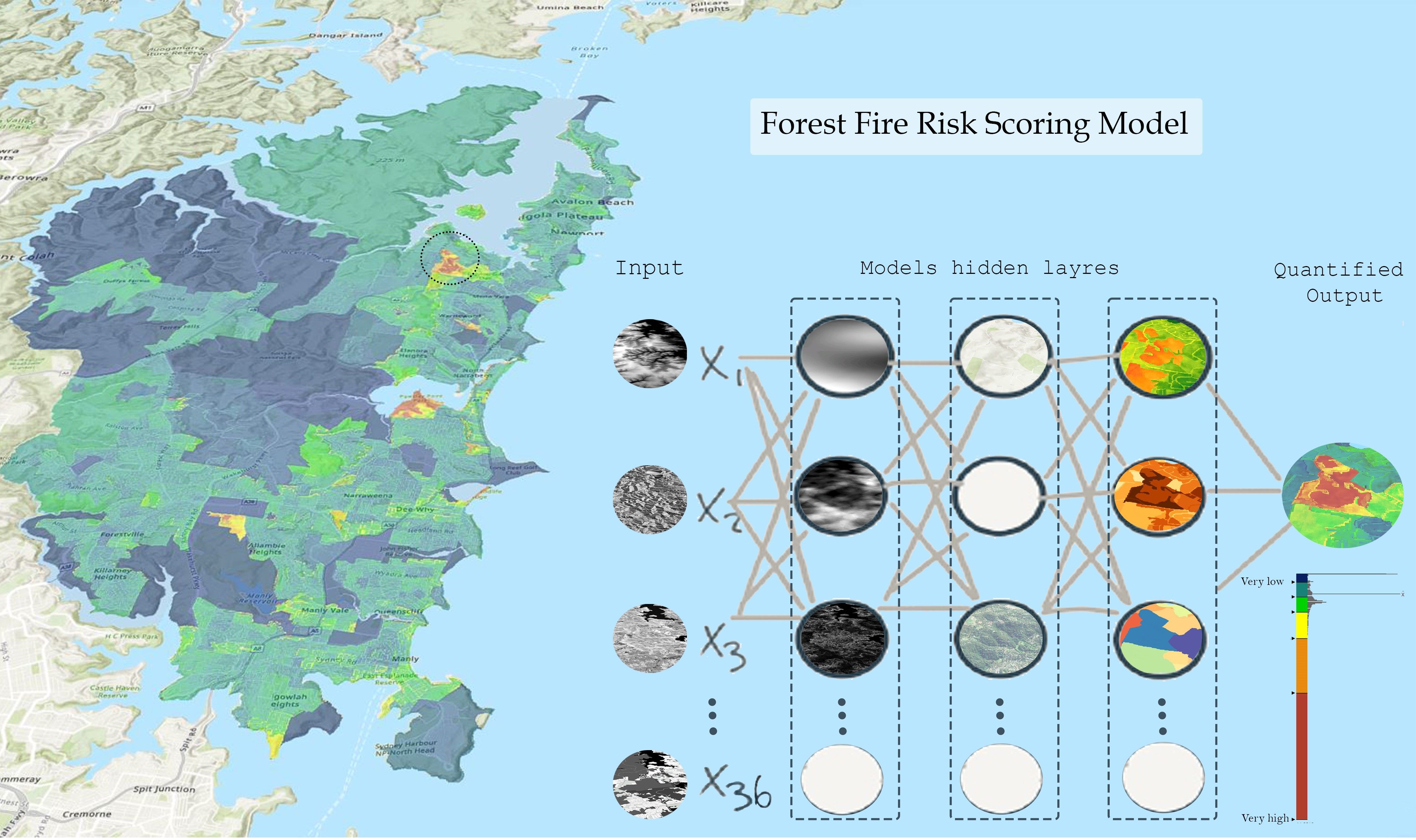
:Forest fire is one of the foremost environmental disasters that threatens the Australian community. Recognition of the occurrence patterns of fires and the identification of fire risk is beneficial to mitigate probable fire threats. Machine learning techniques are recognized as well-known approaches to solving non-linearity problems such as forest fire risk. However, assessing such environmental multivariate disasters has always been challenging as modelling may be biased from multiple uncertainty sources such as the quality and quantity of input parameters, training processes, and a default setup for hyper-parameters. In this study, we propose a spatial framework to quantify the forest fire risk in the Northern Beaches area of Sydney. Thirty-six significant key indicators contributing to forest fire risk were selected and spatially mapped from different contexts such as topography, morphology, climate, human-induced, social, and physical perspectives as input to our model. Optimized deep neural networks were developed to maximize the capability of the multilayer perceptron for forest fire susceptibility assessment. The results show high precision of developed model against accuracy assessment metrics of ROC = 95.1%, PRC = 93.8%, and k coefficient = 94.3%. The proposed framework follows a stepwise procedure to run multiple scenarios to calculate the probability of forest risk with new input contributing parameters. This model improves adaptability and decision-making as it can be adapted to different regions of Australia with a minor localization adoption requirement of the weighting procedure.

1. Introduction
Forest ecosystems are a vital natural resource, providing many economic, social and cultural benefits such as timber, food, fuel, water and air purification, provision of wildlife habitat and recreation; however, forests are regularly under threat by fire [1]. A forest fire, also known as a forest wildfire, bushfire, wildland fire, or vegetation fire, is an unrestrained fire in woodlands, destroying both agricultural lands and built-up areas [2]. The most common causes of forest fire are natural triggers, such as lightning, and actions by humans, such as abandoned barbecue fires, cigarettes, out-of-control burn-offs and sparks from powerlines. Most commonly, forest fires occur during the summer season when dry leaves and fallen sticks are highly flammable [1].
Forest fires have become one of the main concerns in relation to human safety, the environment, and the economy as it results in extreme deforestation and soil erosion and increases the level of CO2 in the ecosystem [3]. Additionally, it negatively impacts forest habitation and the quantity and distribution of tree species. Annually, forest fires destroy 37 million hectares of jungles and forests [3]. Forest fires also destroy infrastructure and property and put human lives at risk [4]. Each year, Australia is seriously threatened by forest fires across the nation. In 2019, the vast national losses due to forest fire include the loss of 34 lives, the destruction of 18.6 million hectares of forest and over 5900 buildings, and the death of one billion animals. Therefore, it is essential to address this disaster by paying more attention to Australia’s forest fire risk management strategy. Due to the increasing occurrence of forest fires, it is necessary to develop an effective framework to manage fire susceptibility, hazard, and risk [1,5].
Forest fire risk assessment is a scientific methodology to quantify risk levels, allowing decision-makers to investigate the trade-offs of alternative actions [6]. It incorporates evidence regarding the likelihood and magnitude of future forest fire events in respect to recent fire behavior such as ignition, spread, suppression, and duration [7]. Without an accurate measure of probable fire risk, it will not be possible to develop a plan to identify and prioritize fire-prone zones [8].
Forest fires, as with any fire, need an ignition triangle consisting of oxygen, heat source, and fuel, such as trees, grasses, dry shrubbery, and forest litter. The main natural sources of ignition are lightning, hot winds, and even the sun. However, in the vast majority of cases, it is human intervention that creates fires, which, under extreme weather conditions, spread uncontrollably [9]. Therefore, incorporating human intervention factors with traditional geospatial variables is a necessity. This paper develops a spatial framework for forest fire risk assessment that incorporates important factors for susceptibility and vulnerability modelling and relies upon new developments in deep learning algorithms to deliver robust, accurate, and useful decision support. The proposed framework is implemented under a geospatial information system (GIS) and evaluated for the Northern Beaches district of Sydney, New South Wales (NSW), Australia.
2. Literature Review
Various research indicates that fire risk assessment is one of the key components in forest fire management [10]. Risk assessment includes the identification of risk and measuring its magnitude and frequency. He et al. [11] categorized forest fire risk assessment into four stages: (a) recognition of hotspot areas, (b) estimation of forest fire susceptibility, (c) identification of areas vulnerable to forest fire, and (d) evaluation of probable forest fire risk.
Environmental factors such as terrain characteristics, human-made infrastructures and meteorological and morphological parameters, referred to as influential parameters, play a significant role in modelling a forest’s susceptibility to fire risk [1]. On the other hand, socio-economic factors contribute to finding the vulnerable areas to zoning the probable risks [12]. A useful platform to incorporate the contributing factors for risk modelling is the geospatial information system (GIS) [5,10], and also cloud computing paradigm with GIS have started to explore scalable frameworks for forest fire [13]. In addition to Geospatial systems, artificial intelligence (AI), machine learning (ML), knowledge-based, and statistical approaches can be employed to assess forest fire risk.
Several studies have investigated how to assess the probability of forest fire risk using remote sensing and GIS structures in conjunction with ML models [3,6,14]. To detect forest fire susceptibility, some studies used knowledge-based approaches, including fuzzy logic, [15], the analytic hierarchy process (AHP) [16], and the analytical network process [17], while others proposed ML approaches, such as neural networks (NNs) [14,18], logistic regression [19], and random forests [20] to a model forest fire. Quantifying a non-linearity problem such as forest fire risk assessment has always been challenging using ML approaches, although NNs have shown an underlying capability to deal with these complex problems [14]. Recently, forecasting the probable locations of any type of disaster has been conducted by integrating GIS and ML technologies [5,21].
To achieve a reproducible and reliable result from ML algorithms, it is necessary to set the hyper-parameters optimized with sufficient training samples. However, these precautions are not usually taken when it comes to regional-scale modelling, which results in simplifying or oversimplifying modelling by applying ML methods compared with the actual results. Forest fire modelling can be biased by multiple sources of uncertainty, including those related to the sampling approach, input parameters, modelling process, and uncalibrated hyper-parameters. Additionally, neglecting significant contributing parameters such as socio-economic indicators may result in the inaccurate estimation of resilience and coping capacity of inhabitants in the event of a forest fire.
3. Forest Fire Risk Prediction Framework
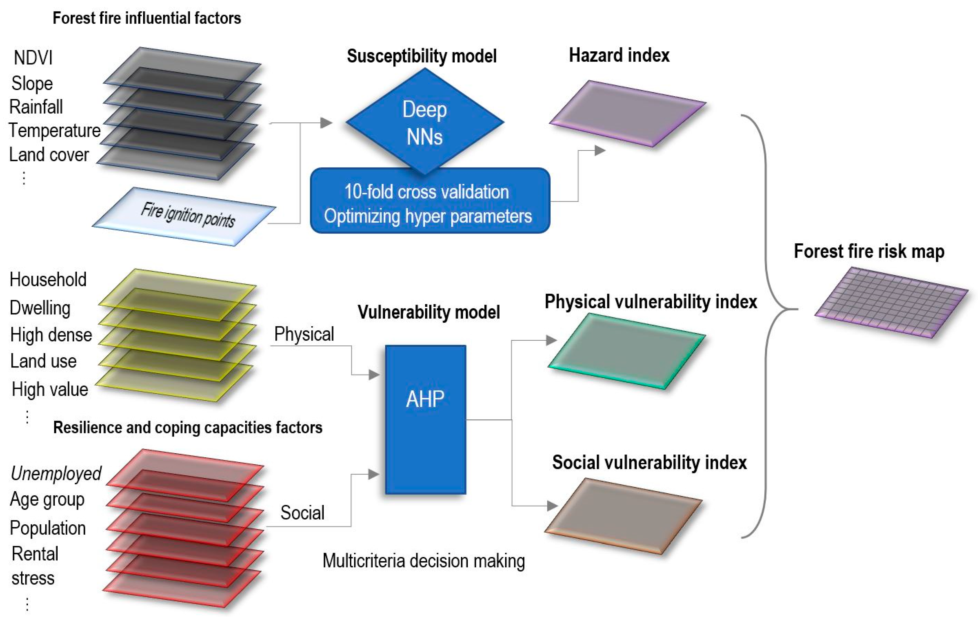
In this study, we set up a framework in which a forest fire risk map can be produced. The framework components are presented in Figure 1. The first stage of this framework is to create 12 contributing factors in relation to forest fire susceptibility analysis. Then, we feed a deep NN with the derived factors to assign a weight to each factor with respect to their influence on forest fire inventory points. In the next step, our deep NN model is optimized via an FbSP optimizer technique. The model runs for 10-fold cross-validation to check the stability of the result. Contributing factors then get overlayed based on the computed weights in the GIS platform to generate a hazard map. A social and physical vulnerability spatial map is generated by the AHP overlay method in raster from 24 socio-economic parameters in the GIS. Finally, a risk function is applied to calculate the forest risk map from the vulnerabilities and hazard maps.
3.1. Contributing Factors
The level of environmental loss due to forest fires is associated with various environmental parameters, including weather and climatic factors, topography, vegetation types, fuel characteristics, and man-made features. These factors influence the intensity and magnitude of forest fires and are usually called contributing parameters [5]. This paper considers twelve important factors from three categories: (1) morphological factors (slope, aspect, NDVI, and altitude), (2) human factors (road density, land cover, distance from the road, and distance from the river), and (3) climatic factors (annual temperature, rainfall, humidity, and wind speed) are selected to evaluate their correlation with the occurrence of forest fire events.
3.2. Susceptibility Model
A susceptibility model needs to be addressed through a systematic methodology based on mathematical models and ML techniques. We apply multivariate assessment methods from ML and AI disciplines to calculate the zones that are susceptible to forest fire based on the historical inventory of forest fire ignition points. To do this, there are four steps of susceptibility assessment through which a hazard map can be generated, namely (a) collecting a forest fire inventory map, (b) deriving the susceptibility contributing parameters, (c) weighting and modelling the parameters using the proposed ML approach, and (d) evaluating the accuracy of the assigned model.
3.2.1. Fire Inventory Map
A fire inventory map contains historical forest fire ignition areas and is one of the main elements of a geospatial database constructed for fire susceptibility modelling [15].
3.2.2. MLP–NN Architect Model
A multilayer perceptron (MLP) is a class of feedforward NN that contains many neurons, which can seamlessly organize input classes into a set of outputs while refining structural models. Once the MLP contains more than three hidden layers, including input and output, it qualifies as deep learning [22]. The NNs comprise reciprocal neurons, which are stabilized into layers with occupied interconnections among hidden layers and produce layers that are required to receive, process, and display the outcome individually. Every layer holds multiple nodes linked by output signals with their associated weights. The weights are generated based on the assigned functions of the summation of the input to the hump prepared by a stimulation turn. The choice of the learning algorithm is the greatest notable circumstance and Backpropagation, which was initially proposed by Werbos [23], is the most common learning algorithm. Backpropagation aims to reduce performance error via the repetitive approach, as shown in Equation (1) [24]:
where signifies the anticipated results, presents the response of vertex in the expected results, and L is the quantity of the vertex in the results. Improvements to weight factors are also designed and produced with the earlier values in the iterative technique, as shown in Equation (2):
where is the weight factors of vertices and ; is a confident constant value responsible for the quantity of modification, which is also known as the learning rate; α is the momentum issue that is given a value between zero and one; indicates the iteration range. Owing to the stabilizing issue, α is cited because it can smoothen fast variations among weights [25].
3.2.3. NNs Model Optimization Process
There are several hyper-parameters that define the robustness of the ML models. The value of these hyper-parameters should be efficiently chosen to achieve the maximum performance of the model [26]. After the nominated hyper-parameters are set for calibration, their desirable domain range should be assigned accordingly. The domain value shows the possible maximum/minimum range for each hyper-parameter. Since the hyper-parameters have an interconnection inside the model, optimum values are subject to test all the domains and their impact on the others; hence, it is a time-consuming procedure to examine all the possible combinations as the genetic algorithm does [27]. Six classes are set for the domain range for the hyper-parameters of our proposed NNs. After selecting the proper domain value associated with each hyper-parameter, the optimizer array is engaged to see all the possible combinations. The fuzzy logic supervised approach (FbSP) is then applied to find the best value for each hyper-parameter so the NNs can achieve better performance [28]. The FbSP optimizes the hyper-parameters in relation to the amount of redundancy between them based on random search methods according to the evaluation metrics. The optimizer starts to run from a random node iteratively to compute the optimal value of the available domain with low inter-correlation [29].
3.2.4. AHP Model
AHP is a multi-criteria decision technique that engages hierarchical structures to represent an issue and then develop priorities for alternatives on the basis of experts’ judgment. The weighting activities in multi-criteria decision making can be effectively dealt with via hierarchical configuration and pairwise comparison table [30]. Pairwise comparisons are based on forming judgements, which were collected from several experts on climate resilience experts and socio-economic specialists. Such comparisons were made between two specific elements rather than attempting to priorities an entire list of elements. The AHP procedures comprise seven parts, namely, construction of a pairwise comparison, normalization of matrix weight, derivation of priority sector, calculation of the maximum eigenvalue, calculation of the consistency index (CI) using eigenvalue, calculation of the random index (RI), and calculation of the consistency ratio (CR). The value of CR should be below 0.1 so that it can be accepted.
3.2.5. Accuracy Assessment Methods
Four well-known accuracy assessment metrics, namely the root mean square error (RMSE), kappa coefficient, receiver operating characteristic (ROC), and precision-recall curve (PRC), are applied against our model to check the precision of the proposed forest fire susceptibility model:
- Kappa coefficient
The K coefficient can measure the overall accuracy of the model, where the total number of correctly assigned samples or the diagonal basics in any error matrix is allocated by the full dataset [31,32,33]. The K coefficient is computed using Equation (3).
where is the total number of rows in the error matrix, is the number of observations of , are the minimal totals, and is the total observation.
- ROC and PRC curves
ROC and PRC curves are designed to assess and visualize the performance of the analytical model. ROC displays sensitivity or the true positive (TP) rate associated with the decision threshold on the y-axis and specificity or false positive (FP) rate on the x-axis [34]. TP can be the positive probability pixel that is classified as it is. In contrast, FP is the negative probability pixel that is also classified as it is. The areas under the ROC curves can be used to estimate the overall accuracy of the model [35,36]. PRC is an additional valuation metric that can support the ROC, particularly when dealing with imbalanced datasets. PRC illustrates the correlation between positive predictive value (PPV) or precision and sensitivity for all possible points, where TP and FP should be calculated. The PRC graph can be plotted by sensitivity over PPV. The x-axis represents recall or sensitivity (), and the y-axis represents precision (). Hence, each point on the PRC graph represents a selected cut-off. The precision and recall that are obtained when this cut-off is chosen are shown. Basically, a perfect model will have an AUC and PRC of 1.
- Root mean squared error (RMSE)
RMSE is a measurement metric evaluating the differences between the predicted model and observed sample values. RMSE signifies the square root of the second trial or the quadratic mean of the variations from the observed examples to the predicted ones using Equation (4) [37]:
where is the testing values, and is the training values at time/place .
3.3. Vulnerability Model
Forest fire vulnerability assessment is characterized as the potential consequence of fire threats while reflecting the resilience and adaptive capacity of the burnt regions [38]. A forest fire vulnerability model also reflects how inhabitants will probably respond and adapt themselves to a fire threat. Usually, a vulnerability model depends on numerous social variables as discussed in other studies, e.g., population, dwelling, age group, unemployment, family, educational qualification, gender, accessibility to services, and housing tenancy [39,40]. These social and physical variables illustrate the existing social inequities among families, which are believed to expand a society’s vulnerability to forest fire hazards [41]. Social vulnerability is the degree to which a person is likely to coping harm due to exposure to the incident, while physical vulnerability reflects the degree to which property or system is likely to experience harm due to exposure to the incident. In this research, 19 social vulnerability indicators and 5 physical vulnerability parameters are chosen based on the living conditions and standards in Australia. Then, the relative significance of the social and physical parameters in relation to forest fires is determined using the analytic hierarchy process (AHP) technique based on an expert’s judgment. In fact, the weightings of the physical and social vulnerability parameters are computed separately based on a pairwise table. Even though different social parameters (e.g., population density, employment rate, and age) might have roughly equal importance in the broad context of vulnerability, their importance is contingent on the type of natural hazard. Then, the consistency index (CI) using eigenvalue, calculation of the random index (RI), and calculation of the consistency ratio (CR) is carried out. The value of CR should be below 0.1 so that it can be accepted. A local socio-economic expert is engaged for this purpose.
3.4. Risk Model
A decent interpretation of forest fire risk assessment is critical to properly manage wildfires [42]. Susceptibility is defined as the likelihood of the incident ignition and the probability of its spreading, and the hazard is the probability of occurrence of the incident within a specified period and within a given area based on the triggering factors, and risk models are the degree of the incident hazard occurrence in a specific area that associated with physical and social vulnerability [20]. After preparing the hazard and vulnerability indices, they are multiplied spatially on the GIS platform using the following equation.
After generating the numerical risk index, it is classified into five classes from very-low to very-high forest fire risk zones using the natural breaks classification technique to make the map easier for interpretation.
4. Implementation and Results
4.1. Study Area
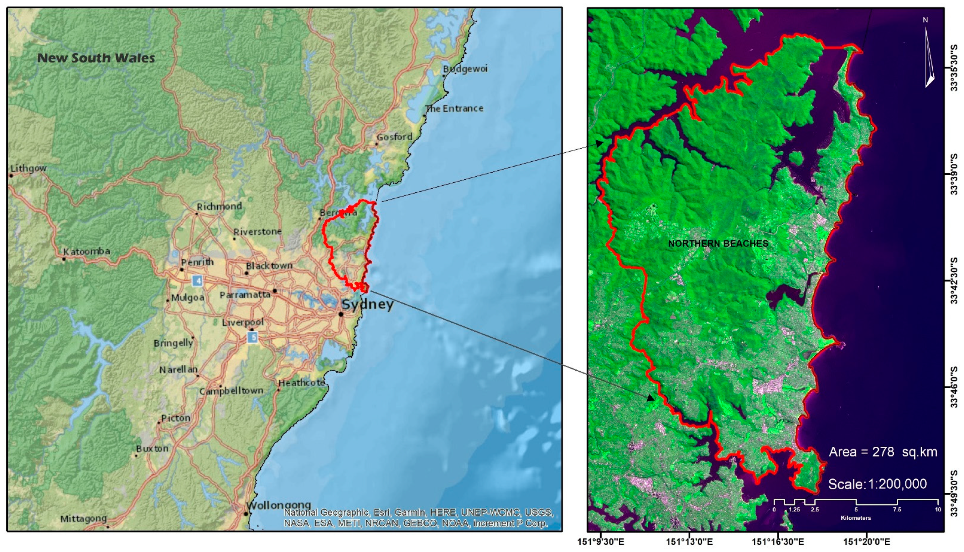
The Northern Beaches area in the state of NSW in Australia has 273,499 inhabitants (census data in 2019) and is the third most populous local government area in Sydney. The Northern Beaches area is mainly a residential and national park, comprising both commercial and industrial areas and rural areas, with a population density of 10.65 persons per hectare. It comprises an area of around 278 km2 from 151.36°E to 33.58°S, including considerable areas of water frontage, coastal foreshores, beaches, islands, national parks, bushland, and reserves. The Northern Beaches area has experienced several forest fires from 2015 till the present, which started in the forest area and extended to the rural and urban areas. Figure 2 shows the location of the study area in the state of NSW.
4.2. Datasets
Meteorological data from the Australian Government Bureau of Meteorology were processed to form climate contributing parameters (http://www.bom.gov.au), Accessed 13 December 2019. The meteorological data measured for the average of two solstices of June 21 and December 21 from 2016 to 2019, including temperature, precipitation, humidity, and wind speed, were collected from 22 nearby gauging stations. Additionally, land cover mesh blocks and topographical data were derived from the NSW government database center in vector or raster formats with a 1-m spatial resolution (https://data.nsw.gov.au), Accessed 5 November 2019. Furthermore, Lidar and Spot-6 images were processed to produce altitude and normalized difference vegetation index (NDVI) maps in 1-m resolution, for two solstices of June (19, 20, and 21) and December (19, 21, and 22) of each year, respectively (https://elevation.fsdf.org.au), Accessed 25 November 2019. Socio-economic data were collected from 2016 and 2020 census records supplied by the Northern Beaches Council to produce spatial vulnerability maps (https://profile.id.com.au/northern-beaches), Accessed 25 November 2019.
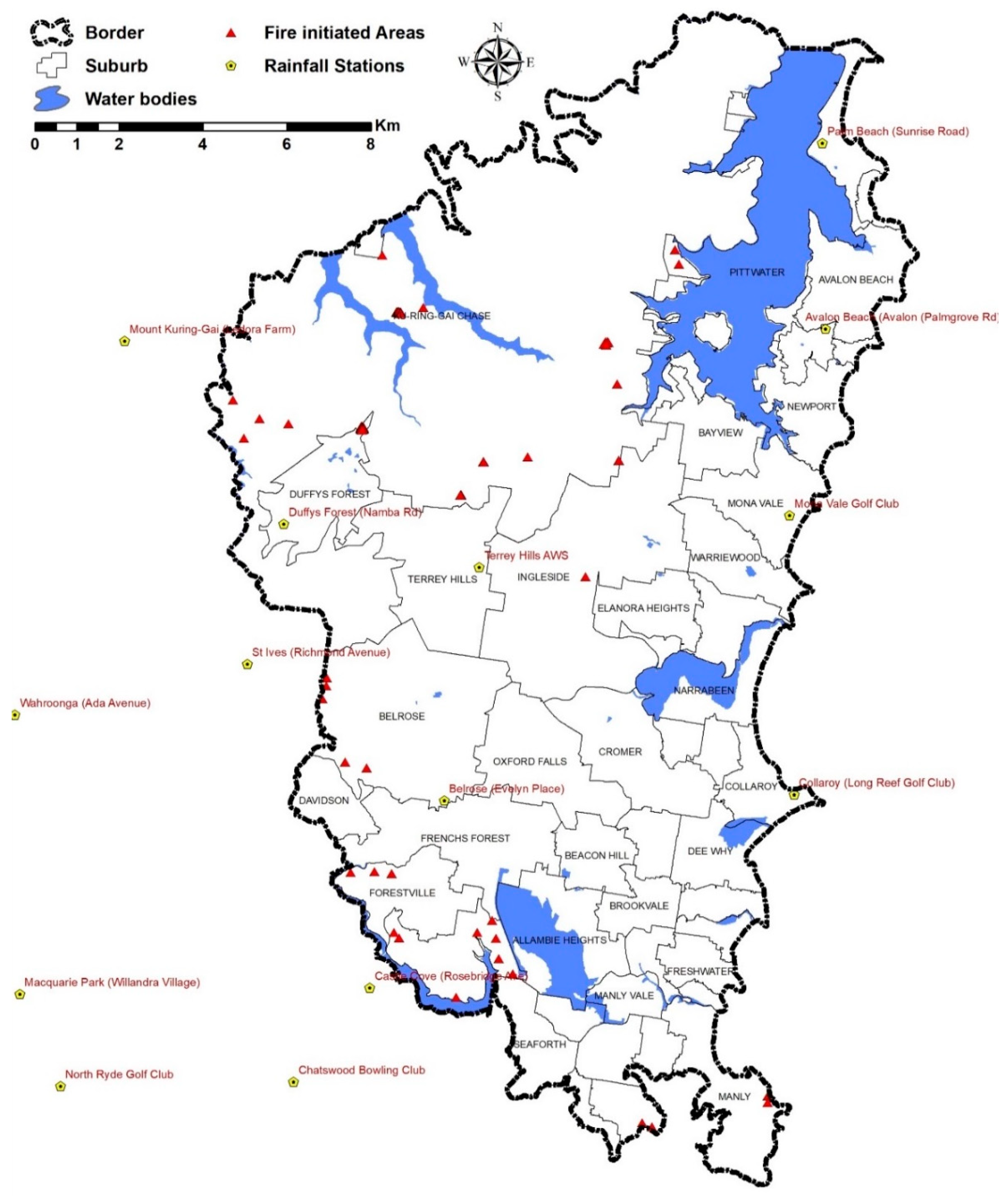
The forest fire inventory map was obtained from the NSW Government using a database of forest fire ignition areas from 2016 to 2019 (see Figure 3). Generally, forest fire ignition is subject to seasonal characteristics. In NSW, spring grass growth can result in an amended outlook with above-normal fire potential. Summer and spring seasons are the most probable seasons for bushfires, which extend from October to May. In November 2019, all states of Australia experienced one of the most severe forest fires, mainly due to extreme weather conditions. For this study, 250 fire ignition points were used to label the training samples. The susceptibility model was trained based on two sets of inventory values of zero and one, where zero indicates the absence of forest fire and one indicates the presence of a forest fire event.
4.3. Contributing factors
In this study, 12 important factors from three categories were selected for modelling forest fire susceptibility.
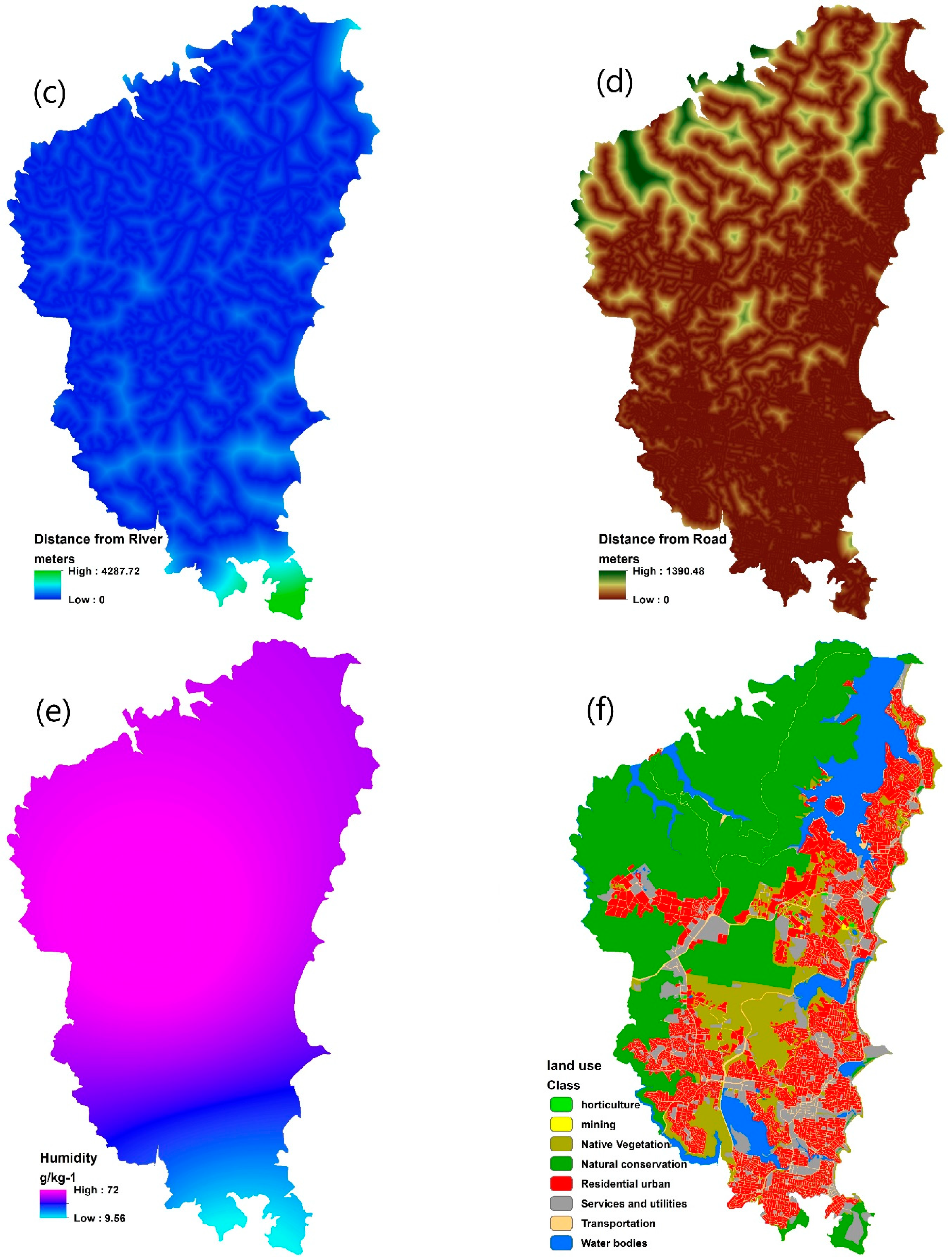
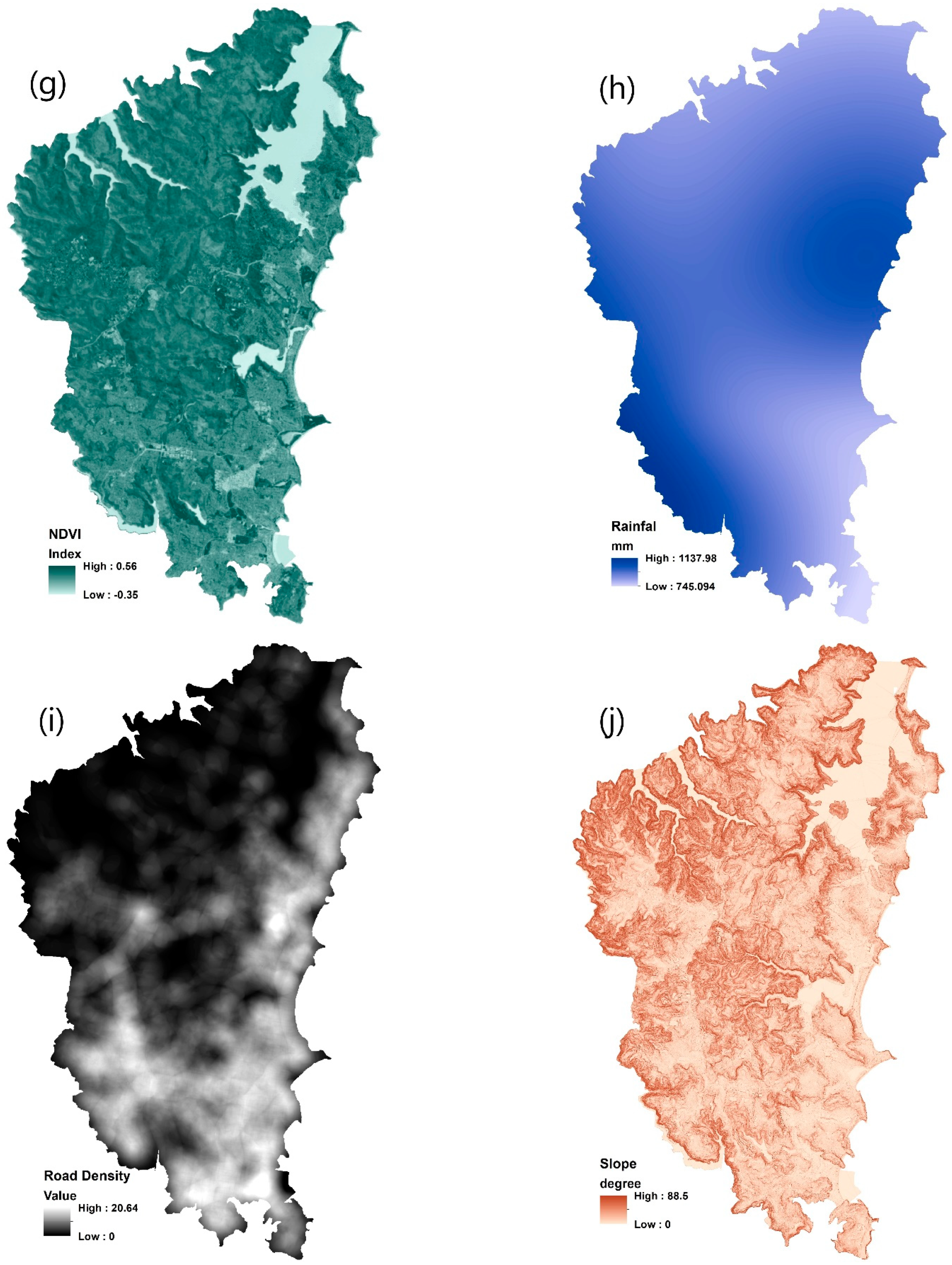
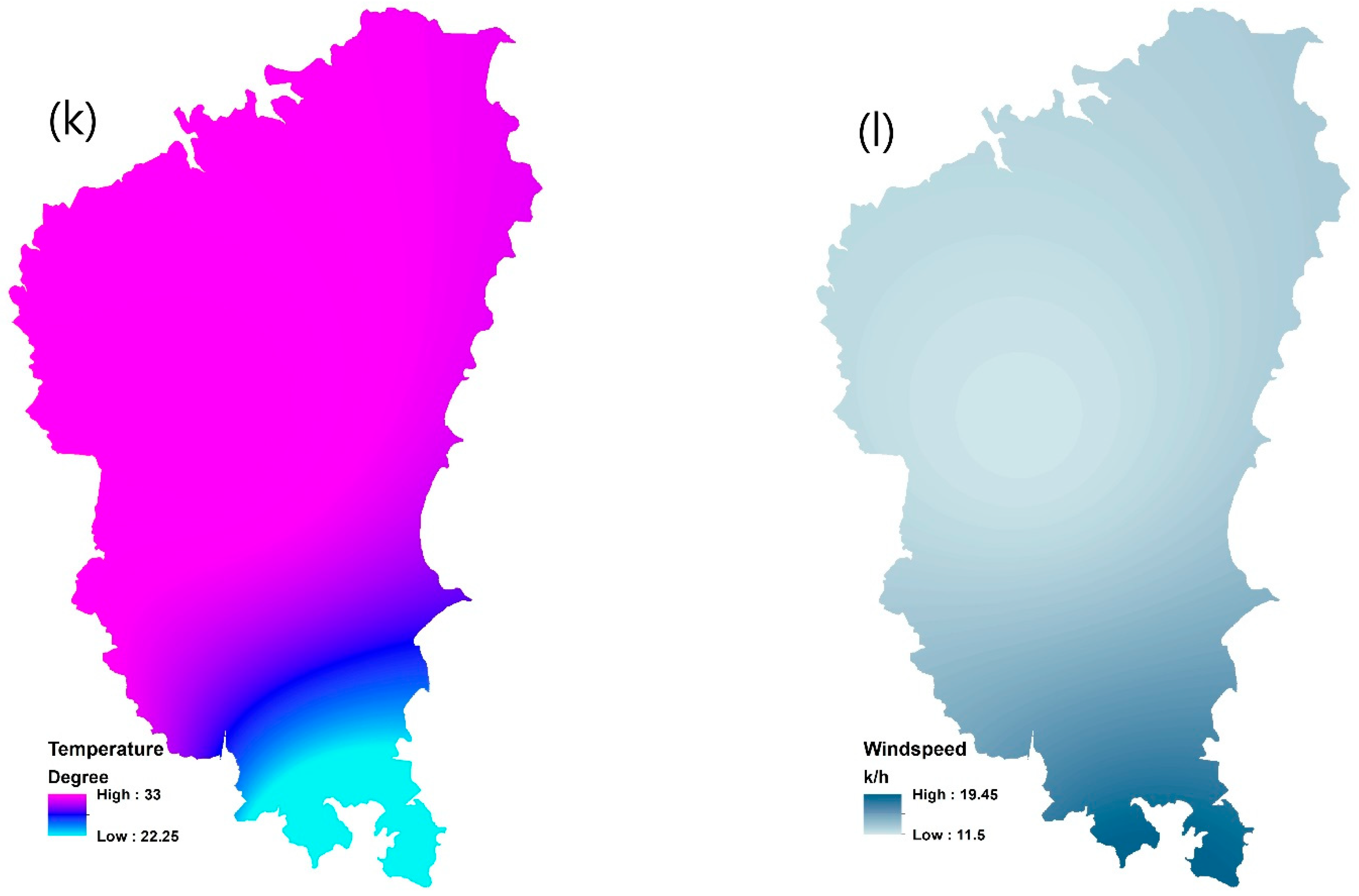
- Climate contributing factors: Weather and climate data were collected from 22 meteorological stations in or near the Northern Beaches area. The spline method was used for integrating them in GIS. The highest and lowest ranges for these layers are spatially mapped in Figure 4. Warmer temperatures, lower relative humidity and precipitation can make the forest surface fuels more sensitive to fire ignition. Wind not only can cut off the soil/surface moisture but also pushes fire flames and sparks into new fuel. Stronger winds supply oxygen to fire, preheating the fuels in the path of the fire. When hot, dry, and windy conditions happen at the same time, fire ignition can be occurred and spread quickly.
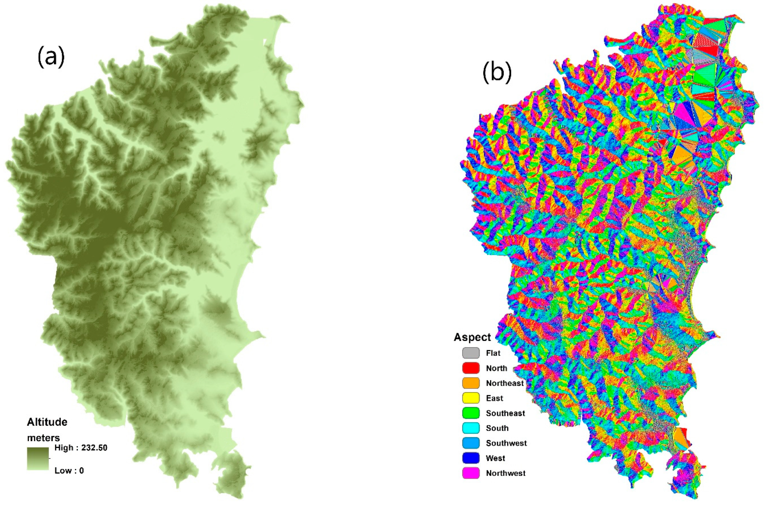
- Human-induced contributing factors: Human activity is one of the main causes of forest fire, with most fires being triggered near roads, camping parks, riverbanks, etc. Hence, we spatially mapped some of the key factors in this category, such as road density, land cover, distance from the road, and distance from the river. Euclidian distance analysis was applied on the road and river networks to rasterize these approximate maps. Density analysis was used to calculate road density, and a land cover map was converted to a raster format to represent the general typology coverage, including natural conservation, native vegetation, water bodies, services and utilities, transportation, horticulture, mining, and residential urban.
- Physical contributing factors: Four key physical contributing factors in relation to forest fire are investigated in this study, namely altitude, NDVI, aspect, and slope. The altitude was generated from a LiDAR point cloud. NDVI was generated from the red and infrared bands of the Spot-6 satellite image. The highest and lowest ranges for these layers are spatially mapped in Figure 4.
4.4. Vulnerability Model
For vulnerability modelling, 19 social indicators and 5 physical parameters were chosen based on the living conditions and standards in the Northern Beaches area as follows.
4.4.1. Social factors
These factors reflect how the inhabitant may cope with a disaster such as a forest fire. They also provide deep information about people’s resilience against forest fire hazards. This information was collected from the Northern Beaches Council in a tabular format in the scale of statistical areas level 1 (SA1). We then spatially mapped them from the mesh blocks as geographical areas, including the following 19 indicators:
- The rental population: The housing tenure demographic can provide insights into the resident’s socio-economic status. For instance, a large number of renters in a particular area might indicate that the housing affordability in that area may attract low-income young people who wish to buy a house, whereas a high number of homeowners in a particular area might indicate it is a more settled area where the population is less socially vulnerable. Additionally, tenure data might indicate built form distribution, where a higher concentration of renters indicates many high-density dwellings whereas a lower concentration of renters indicates the presence of homeowners living in separate houses.
- Families without a car: A family’s access to public services and health facilities can be affected by their access to the public/private transport system. The number of vehicles per family indicates accessibility to private transport and indirectly reflects those who need to access the public transportation system. Therefore, car ownership is an indicator to measure how quickly families can react to an evacuation in the case of a fire. Families without a car are more vulnerable to hazard such as a forest fire as they need to find a vehicle to vacate fire-affected areas.
- Rental stress: Families whose incomes are in the bottom 40% of the population and who spend more than 30% of their weekly income on rent are said to be suffering rental stress.
- Unemployment: Unemployment data is one of the most important socio-economic parameters that indicate the ability of the family to cope with unexpected events. The unemployment rate indicates the number of individuals looking for jobs as a ratio of the labor force. Families with a higher unemployment rate may not have savings, which makes them more vulnerable to disasters such as forest fires.
- Families with no educational qualification: Educational qualifications are one of the most important indicators of socio-economic status. This parameter identifies the number of people aged over 15, who have not finished high school, or their qualifications are not recognized in Australia. Individuals without any recognized qualifications tend to be disadvantaged as Australian employers tend to require formal qualifications. These families might face difficulties finding well-paid jobs and are hence more vulnerable when faced with a disaster event.
- Families with a disabled member: This parameter identifies families who have a family member who requires support and assistance in their daily lives with self-care, communication, or body movement due to a disability, health illness, or old age. This parameter indicates the number of families who may not be able to evacuate an area quickly in the event of a disaster; hence, they are classified as highly vulnerable in natural disasters.
- Low-income families: Low-income families, defined as those whose income is less than $650 per week, may not have sufficient savings, which makes them vulnerable in the event of a disaster. Household income is one of the most important indicators of socio-economic status. Low-income families then are more vulnerable to forest fires as they are not resilient to disaster.
- Older lone persons: Older lone person households often indicate an area that has been through its suburb life cycle and now mainly consists of an elderly population that needs relevant support services. The type of household and family structure of the population are important indicators. It generally shows the vulnerable areas and provides strategic awareness to the degree of request for facilities and services in case of emergency and hazard.
- Newly arrived families from overseas: This parameter indicates the spatial distribution of foreigners who recently arrived in Australia. These families usually do not have comprehensive information about their neighborhood of residence or the surrounding environment, and they are also probably unfamiliar with the likelihood of potential disaster, which makes them vulnerable in a disaster event.
- Parents with a child under 15: Generally, families with dependent children are more vulnerable than families without dependent children in the case of fire evacuations.
- Single parent with a child under 15: In general, households with children need more services and emergency facilities than other household types, and their needs tend to be dependent on the children’s age. Single-parent families with dependent children are much more vulnerable to natural disasters than couple families with dependent children, particularly in the case of a fire evacuation. Understanding spatial socio-economic information can help urban planners make evidence-based decisions about the allocation of emergency response centers.
- Families with members in a vulnerable age group: Identifying the population in the vulnerable age group is an indicator of a low coping capacity in the event of a disaster. The age structure of a population is usually indicative of an area’s life cycle stage and provides key insights into the level of demand for age-specific services and facilities. Children under 15 years or people aged above 60 are considered dependent populations who need assistance in the case of a forest fire.
- Population: Population is one of the key indicators for vulnerability assessment. Those areas with a large population need to have emergency contingency plans in place in the event of a disaster. In this study, population data were demographically mapped at the mesh block level for the Northern Beaches area and is combined with other basic demographic information, such as gender and age structure.
- Population density: Population density indicates the average number of persons per hectare in our study area. The population density indicator might be misleading as some of the regions might not be used for residence. Basically, areas with highly populated residential housing have a higher density value than areas where most of the land is used for other purposes such as industry or parkland.
4.4.2. Physical Vulnerability
These factors highlight valuable properties and households where more protection and percussion against forest fire disasters are needed. They also provide deep information about spatial susceptible hot spots that might cause irremediable damage to society in case of hazard. This information was collected from the Northern Beaches Council in a tabular format and then spatially mapped into geographical areas, including the following five indicators:
- High-density housing: The residential built form often reflects planning policy, such as building denser forms of housing around public transport nodes or employment centers. A greater concentration of flats, units, and apartments will accommodate more of the population. This indicator shows high-density dwellings, which include flats that are three or more stories high. High-density housing is common in inner-city areas and some suburban areas close to railway stations, as well as some coastal resorts. This type of housing has increased in popularity in Australia in recent years.
- Number of households: The number of households is one of the informative indicators that show high/low populated neighborhoods. It indicates a house and its occupants regarded as a unit. Average household size is calculated by dividing the number of occupied dwellings by the total number of inhabitants.
- Dwellings: The location of dwellings represents people’s assembly points across the night and part of a day. Therefore, the spatial mapping of dwellings can also help us to zoom down up to the vital areas that have to be preserved in terms of hazard. It is very essential to implement protective actions such as biological and mechanical plans to save human lives gathered in dwellings.
- High rental dwellings: High rental is defined as a rental payment of more than $600 per week in this study. High rental payments may indicate desirable areas with mobile populations who rent, or a housing shortage, or gentrification. Low rental payments may indicate public housing or areas where there are many low-income households looking for a lower cost of living. However, rental payments are not directly comparable over time because of inflation.
- Land usage: The land use was ranked from zero to one regarding the degree of physical importance, rehabilitation and heritage to the community, as summarized in Table 1. Zero indicates low vulnerable land zone uses, and one indicates highly vulnerable land use zones.
4.5. Results Analysis
4.5.1. Model Training and Finetuning
Most ML-based models have several hyper-parameters that must be calibrated precisely to achieve the ideal outcome. The hyper-parameters have their own upper and lower range called the domain. To optimize the model, not only must all the possible domains of each hyper-parameter be examined but also the interaction between the hyper-parameters needs to be considered. Retrieving the ideal value for the hyper-parameters of the ML models using trial and error is a tedious and time-consuming procedure that mostly leads to inaccurate results, particularly when dealing with more than four hyper-parameters with wide domain ranges. Hence, automating the selection of the optimal value is a suitable solution to decrease computational time and increase the accuracy of the final output by considering all possible interactions between the hyper-parameters. The FbSP optimizer technique examines the influence of various hyper-parameters on the model attributes. In this study, the deep NN model with MLP architecture was optimized through the FbSP over 100 iterations. The optimization algorithm initiates superior configurations at any iteration until convergence. However, using many iterations may not necessarily result in enhanced configurations. Thus, we found the optimal hyper-parameter values over the 100 iterations, which improved the accuracy of MPL–NN using 10-fold cross-validation. Table 2 details the feasible hyper-parameters of the implemented models and the ideal value for each.
The MLP–NN model achieved the best performance after tuning its six hyper-parameters, including the number of hidden layer attributes, hidden layer classes, learning rate, momentum, seed number, and batch size. The well-tuned MLP–NN architecture solved the bias and variance reduction of the basic MLP. As three of the NN’s hidden layers and classes were used, deep NNs achieved a lower error rate.
Based on the MLP−NN calculation, negative values for parameters show an indirect relationship to fire susceptibility, while positive values indicate a direct relationship. For example, wherever there was a lower value for rainfall, the probability of fire increased. On the other hand, the magnitude weight of parameters indicates their significant correlation with forest fire, whether negative or positive, see Figure 5. Therefore, road density was influential to forest fire followed by distance from the river, land cover typology, and NDVI as −0.077, +0.050, −0.049, and +0.045, respectively. In other words, variation in the value of the mentioned parameters is extremely synchronized with the present r absence of forest fire initiation. However, other parameters showed a moderate correlation with forest fire, including slope, rainfall, humidity, wind speed, and temperature, in our study area. Distance from river, aspect, and altitude received the lowest contribution degree as +0.001, −0.034, and −0.009, respectively.
For training and testing, the 10-fold cross-validation method was used. Therefore, 10% of the total incidents for each iteration were used for testing, and the remainder was used for training. This approach rotated over different incidents for the next iteration. Therefore, we avoided bias error by randomly dividing the incidents into testing and training (e.g., 30% and 70%) prior to running the model. After the completion of the testing and training, the multiple evaluation matrix was examined against our results showing high precision and accuracy in classifying the incidents as summarized in Table 3. ROC = 95.1%, PRC = 93.8%, k coefficient = 94.3%, and RMSE = 0.165, which is quite substantial in this field. Consequently, the deep NN model was trained well with all the contributing parameters regarding the inventory ignition of fires to successfully predict high/low forest fire susceptibility zones.
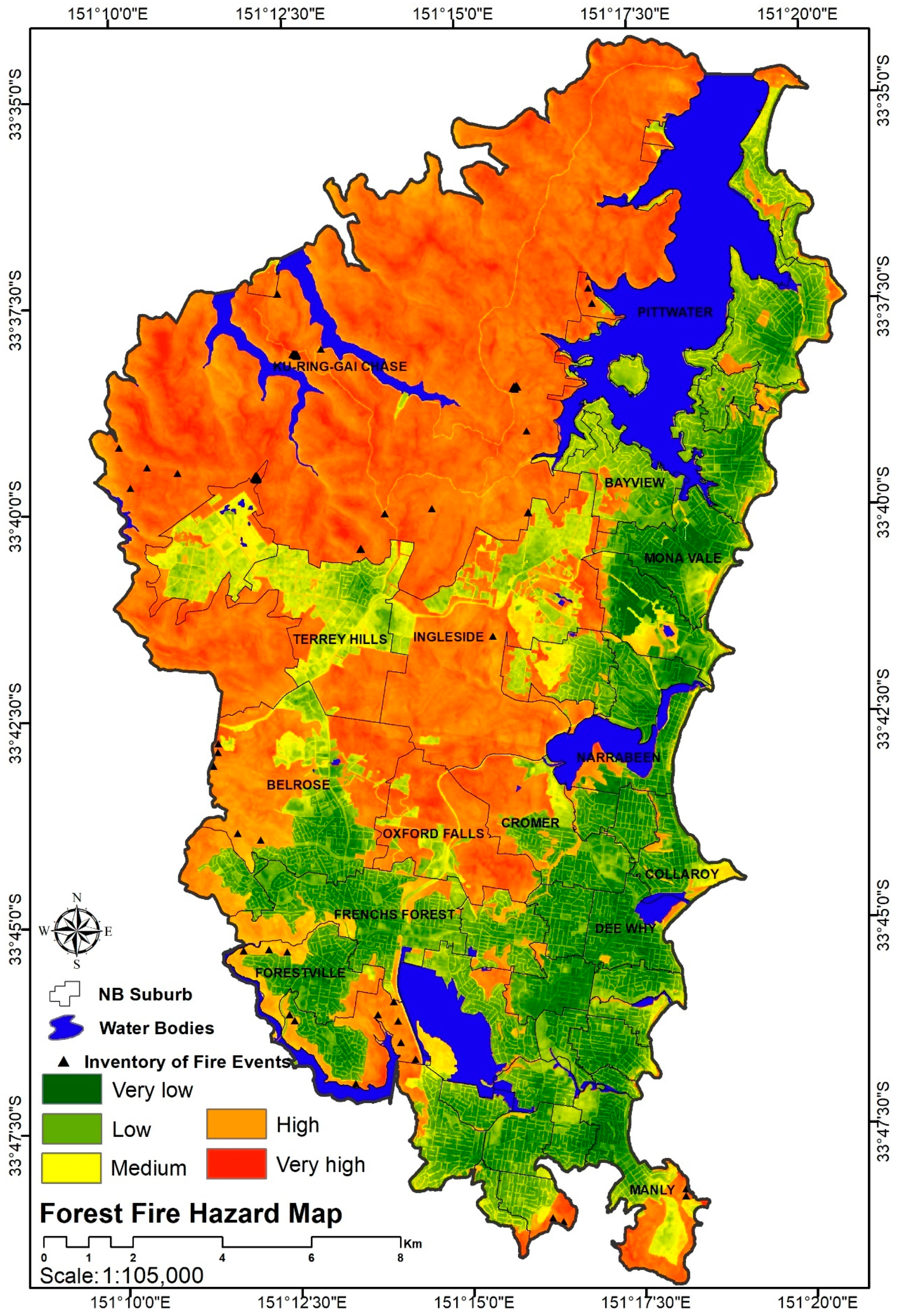
4.5.2. Forest Fire Hazard Index
A low precipitation rate in the region increased the susceptibility of the forest fire ignition compared to other climate parameters. Though steep land is commonly more prone to forest fires, the land cover layer was a significant factor in susceptibility to a forest fire. Suburbs close to Ku-ring-gai Chase National Park, such as Oxford Falls, are predominantly covered by forest and dense vegetation and are therefore categorized as very high forest fire hazard zones due to the nature of wildfire.
Residential and built-up areas in several suburbs, such as Duffy’s Forest, Terrey Hills, and Ingleside, fell into the high hazard zones as represented in yellow in Figure 6, whereas only parts of other suburbs, such as Elanora Heights, Manly, and Belrose, fell into the high hazard zones, refer to Figure 6.
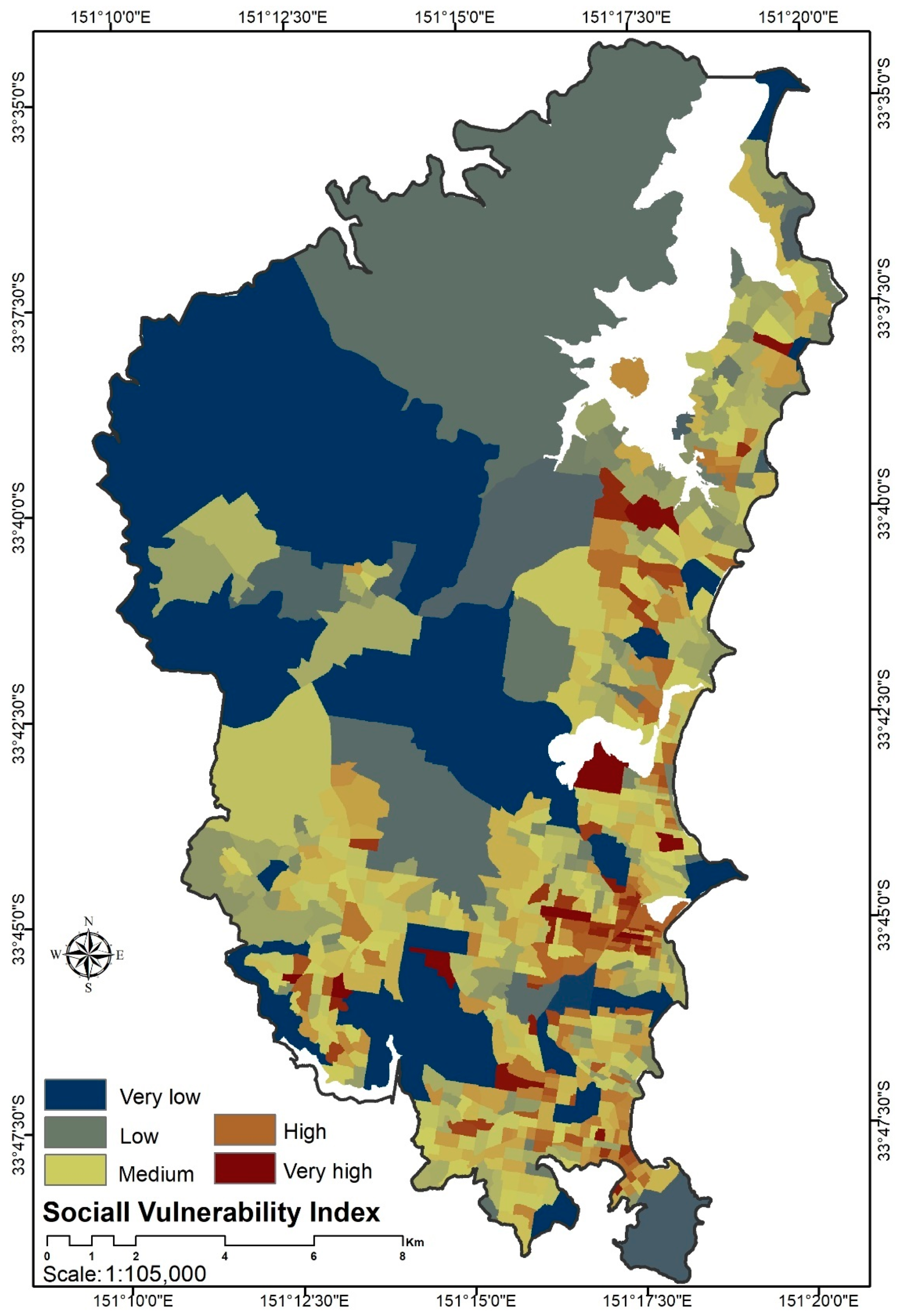
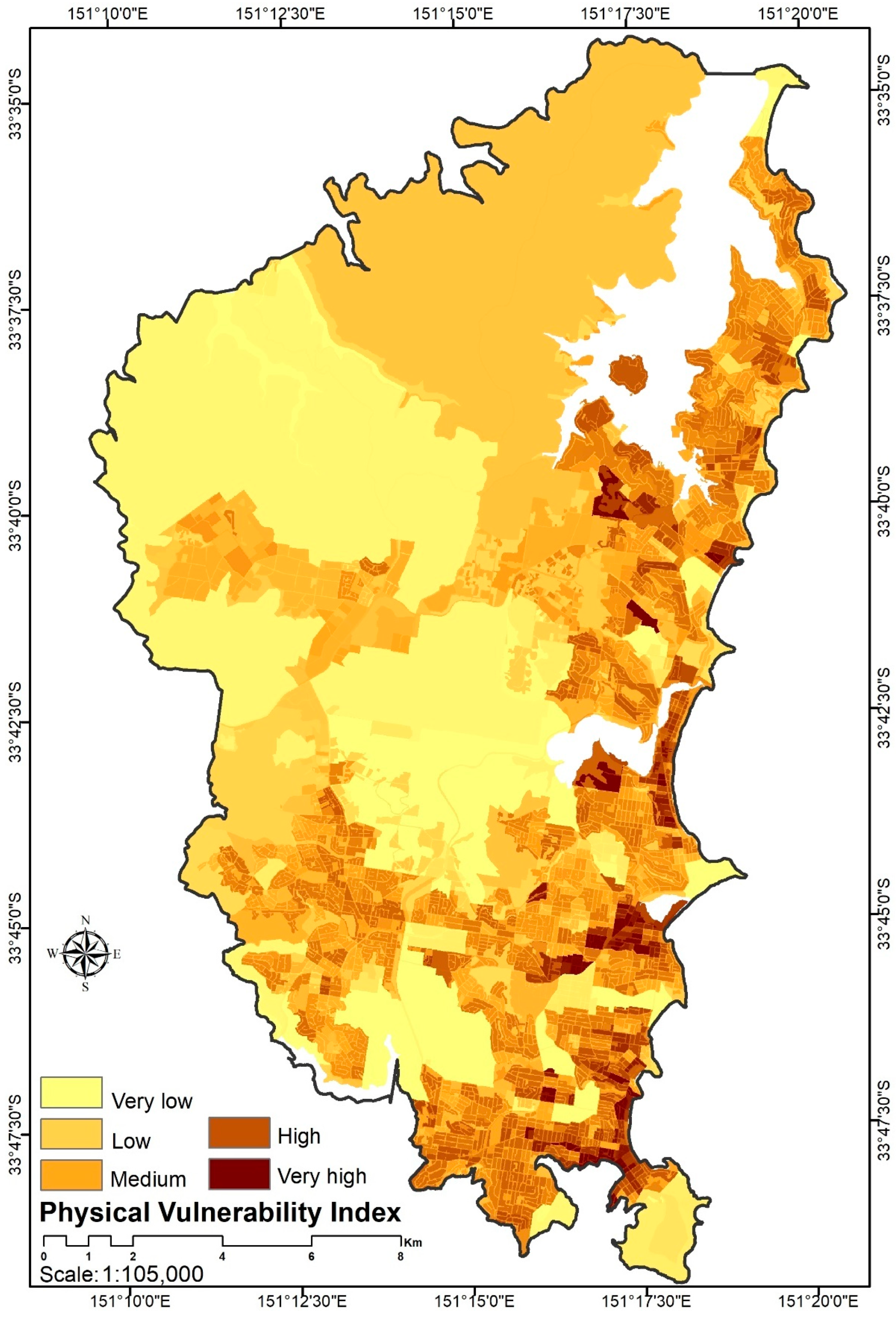
4.5.3. Forest Fire Vulnerability
To create vulnerability maps through the AHP approach, we computed the pairwise table matrices to prioritize the social and physical parameters based on the expert’s opinion, who was a specialist in forest fire management and socio-economic fields. Both the pairwise comparison matrices of social and physical vulnerability passed the consistency test with overall CR scores of 0.012 and 0.004, respectively. The achieved weights associated with the indicators are presented in Table 4.
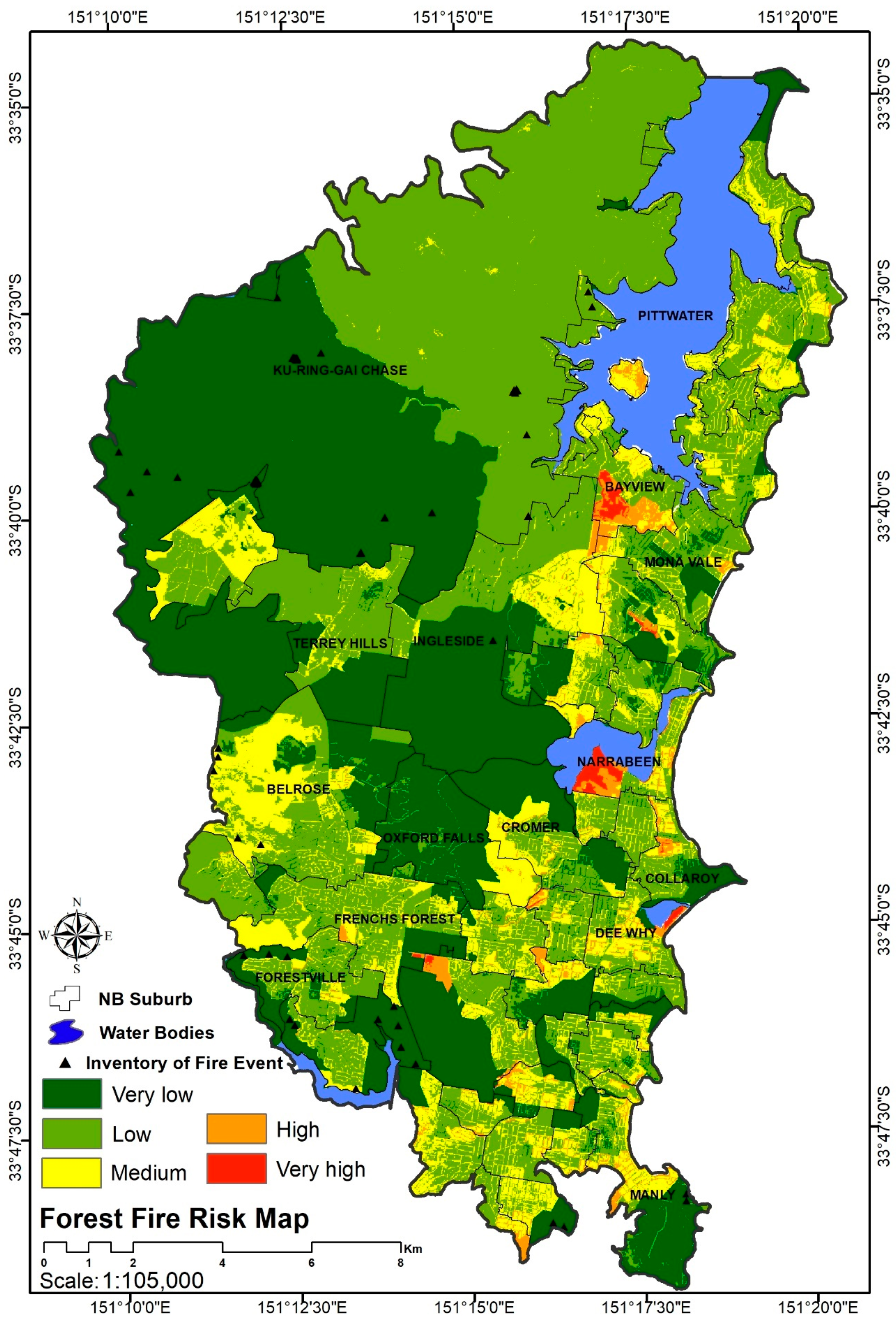
4.5.4. Forest Fire Risk Level
Using the outputs of both susceptibility and vulnerability models, the framework produced the risk levels for the area, as shown in Figure 9. Generally, less than 2.5% of the Northern Beaches area is classified as being very high- or high-risk zones in relation to forest fire (504 hectares). Almost 84% of the area under study is in a safe zone of very low to low risk. Approximately 14% of the area investigated by this study is in a medium risk zone, as presented in Table 5.
As can be seen from Figure 9, although areas of Ku-ring-gai Chase that are close to the national park and the suburbs of Oxford Falls, Terrey Hills and Ingleside are categorized as a very high hazard zone, they are not in a forest fire risk zone. After applying the social and physical vulnerability layers on the hazard index, areas that are at risk of forest fire are highlighted. Narrabeen and Bayview are in very risky zones and require a practical forest fire reduction plan.
5. Discussion
The main brain running this proposed spatial framework, which is the deep NN model with MLP architecture, was optimized through the FbSP to achieve the best possible outcome yet not lean towards overfitting. There are, however, some ancillary environmental factors that could use besides the current ones as inputs of this forest fire risk model, such as soil moisture, which will be considered for our future assessment. The proposed spatial framework can run multiple scenarios to calculate the probability of forest risk with updated contributing parameters. For example, the construction of new buildings near the national park increases the degree of risk to those neighbors’ cells accordingly. In another scenario, any changes in socio-economic demography can result in an increase/decree of resilience and then alter the degree of vulnerability that directly influences the quantity of probable risk for that area.
6. Conclusions and Future Works
The spatial assessment of forest fire risk, which threatens human lives and property, is an important part of land emergency management, mitigating the impact of natural hazards, and firefighters’ response and recovery. It helps to assess forest fire risk and improves adaptability and decision making. This paper developed a risk assessment framework based on the capabilities of the deep neural network model. The framework generates risk levels based on the susceptibility and vulnerability models. Several geospatial variables are used for susceptibility modelling, and several socio-economic parameters are utilized for social and physical vulnerability modelling. The proposed framework can be adapted to different regions of Australia and other world areas with minor localization adoption using a weighting procedure. The framework can be updated by streaming temporal updates of contributing parameters over time. The performance of the framework was evaluated in a case study, the Northern Beaches of NSW, Australia. Future studies will consider more in-depth morphological parameters such as forest biodiversity, soil moisture, tree specification, and conditions to examine their contribution to forest fire hazard assessment. Additionally, it would be worthwhile examining and comparing other state-of-the-art ML models such as gradient boosting, convolutional neural networks, or ensemble approaches.
Author Contributions
Conceptualization, M.N.; Formal analysis, F.R.; Funding acquisition, M.N.; Investigation, M.N.; Methodology, H.M.R.; Project administration, M.N.; Resources, F.R.; Software, F.R.; Validation, H.M.R.; Writing—original draft, H.M.R.; Writing—review & editing, M.N. and F.R. All authors have read and agreed to the published version of the manuscript.
Funding
This research received no external funding.
Informed Consent Statement
Not applicable.
Data Availability Statement
For this study, we have use open source and governmental dataset from these addresses: Meteorological data from the Australian Government Bureau of Meteorology (http://www.bom.gov.au, accessed on 25 November 2019). Cadastral and topographical data from the NSW government database center (https://data.nsw.gov.au, accessed on 25 November 2019). Satellite images (https://elevation.fsdf.org.au, accessed on 25 November 2019). Socio-economic census data from the Northern Beaches Council (https://profile.id.com.au/northern-beaches, accessed on 25 November 2019).
Conflicts of Interest
The authors declare no conflict of interest.
References
- Said, S.N.B.M.; Zahran, E.-S.M.M.; Shams, S. Forest fire risk assessment using hotspot analysis in GIS. Open Civ. Eng. J. 2017, 11, 786–801. [Google Scholar] [CrossRef]
- Pearce, D.W. The economic value of forest ecosystems. Ecosyst. Health 2001, 7, 284–296. [Google Scholar] [CrossRef]
- Ajin, R.; Ciobotaru, A.; Vinod, P.; Jacob, M.K. Forest and Wildland fire risk assessment using geospatial techniques: A case study of Nemmara forest division, Kerala, India. J. Wetl. Biodivers. 2015, 5, 29–37. [Google Scholar]
- Vadrevu, K.P.; Eaturu, A.; Badarinath, K. Fire risk evaluation using multicriteria analysis—A case study. Environ. Monit. Assess. 2010, 166, 223–239. [Google Scholar] [CrossRef] [PubMed]
- Naderpour, M.; Rizeei, H.M.; Khakzad, N.; Pradhan, B. Forest fire induced Natech risk assessment: A survey of geospatial technologies. Reliab. Eng. Syst. Saf. 2019, 191, 106558. [Google Scholar] [CrossRef]
- Calkin, D.E.; Ager, A.; Thompson, M.P.; Finney, M.A.; Lee, D.C.; Quigley, T.M.; McHugh, C.W.; Riley, K.L.; Gilbertson-Day, J.M. A Comparative Risk Assessment Framework for Wildland Fire Management; The 2010 Cohesive Strategy Science Report; National Agroforestry Center: Lincoln, NE, USA, 2011.
- Sikder, I.U.; Mal-Sarkar, S.; Mal, T.K. Knowledge-based risk assessment under uncertainty for species invasion. Risk Anal. Int. J. 2006, 26, 239–252. [Google Scholar] [CrossRef] [PubMed]
- Ager, A.A.; Finney, M.A.; Kerns, B.K.; Maffei, H. Modeling wildfire risk to northern spotted owl (Strix occidentalis caurina) habitat in Central Oregon, USA. For. Ecol. Manag. 2007, 246, 45–56. [Google Scholar] [CrossRef]
- Naderpour, M.; Rizeei, H.M.; Ramezani, F. Wildfire prediction: Handling uncertainties using integrated bayesian networks and fuzzy logic. In Proceedings of the 2020 IEEE International Conference on Fuzzy Systems (FUZZ-IEEE), Glasgow, UK, 19–24 July 2020; pp. 1–7. [Google Scholar]
- Sivrikaya, F.; Sağlam, B.; Akay, A.E.; Bozali, N. Evaluation of forest fire risk with GIS. Pol. J. Environ. Stud. 2014, 23, 187–194. [Google Scholar]
- He, Y.; Lin, Y.; Wu, M. The effect on organizational performance by human resource management practices: Empirical research on Chinese manufacturing industry. In Proceedings of the 2010 International Conference on Management and Service Science, Wuhan, China, 24–26 August 2010; pp. 1–6. [Google Scholar]
- Alexakis, D.; Sarris, A. Environmental and human risk assessment of the prehistoric and historic archaeological sites of Western Crete (Greece) with the use of GIS, remote sensing, fuzzy logic and neural networks. In Proceedings of the Euro-Mediterranean Conference, Lemessos, Cyprus, 8–13 November 2010; pp. 332–342. [Google Scholar]
- Garg, S.; Aryal, J.; Wang, H.; Shah, T.; Kecskemeti, G.; Ranjan, R. Cloud computing based bushfire prediction for cyber–physical emergency applications. Future Gener. Comput. Syst. 2018, 79, 354–363. [Google Scholar] [CrossRef] [Green Version]
- Ghorbanzadeh, O.; Blaschke, T.; Gholamnia, K.; Aryal, J. Forest fire susceptibility and risk mapping using social/infrastructural vulnerability and environmental variables. Fire 2019, 2, 50. [Google Scholar] [CrossRef] [Green Version]
- Pourghasemi, H.R.; Beheshtirad, M.; Pradhan, B. A comparative assessment of prediction capabilities of modified analytical hierarchy process (M-AHP) and Mamdani fuzzy logic models using Netcad-GIS for forest fire susceptibility mapping. Geomat. Nat. Hazards Risk 2016, 7, 861–885. [Google Scholar] [CrossRef] [Green Version]
- Suryabhagavan, K.; Alemu, M.; Balakrishnan, M. GIS-based multi-criteria decision analysis for forest fire susceptibility mapping: A case study in Harenna forest, southwestern Ethiopia. Trop. Ecol. 2016, 57, 33–43. [Google Scholar]
- Ghorbanzadeh, O.; Blaschke, T. Wildfire susceptibility evaluation by integrating an analytical network process approach into GIS-based analyses. In Proceedings of the ISERD International Conference, Tehran, Iran, 11–12 July 2019. [Google Scholar]
- Dutta, R.; Das, A.; Aryal, J. Big data integration shows Australian bush-fire frequency is increasing significantly. R. Soc. Open Sci. 2016, 3, 150241. [Google Scholar] [CrossRef] [PubMed] [Green Version]
- Kuter, N.; Yenilmez, F.; Kuter, S. Forest fire risk mapping by kernel density estimation. Croat. J. For. Eng. J. Theory Appl. For. Eng. 2011, 32, 599–610. [Google Scholar]
- Kim, S.J.; Lim, C.-H.; Kim, G.S.; Lee, J.; Geiger, T.; Rahmati, O.; Son, Y.; Lee, W.-K. Multi-temporal analysis of forest fire probability using socio-economic and environmental variables. Remote Sens. 2019, 11, 86. [Google Scholar] [CrossRef] [Green Version]
- Mojaddadi, H.; Pradhan, B.; Nampak, H.; Ahmad, N.; Ghazali, A.H.b. Ensemble machine-learning-based geospatial approach for flood risk assessment using multi-sensor remote-sensing data and GIS. Geomat. Nat. Hazards Risk 2017, 8, 1080–1102. [Google Scholar] [CrossRef] [Green Version]
- Neupane, B.; Horanont, T.; Aryal, J. Deep learning-based semantic segmentation of urban features in satellite images: A review and meta-analysis. Remote Sens. 2021, 13, 808. [Google Scholar] [CrossRef]
- Werbos, P. Beyond regression: New tools for prediction and analysis in the behavior science. Unpubl. Dr. Diss. Harv. Univ. 1974, 10019522029. [Google Scholar]
- Mia, M.; Dhar, N.R. Prediction of surface roughness in hard turning under high pressure coolant using Artificial Neural Network. Measurement 2016, 92, 464–474. [Google Scholar] [CrossRef]
- Yang, W.T.; Ahuja, A.; Tang, A.; Suen, M.; King, W.; Metreweli, C. Ultrasonographic demonstration of normal axillary lymph nodes: A learning curve. J. Ultrasound Med. 1995, 14, 823–827. [Google Scholar] [CrossRef]
- Liao, S.-H.; Chu, P.-H.; Hsiao, P.-Y. Data mining techniques and applications–A decade review from 2000 to 2011. Expert Syst. Appl. 2012, 39, 11303–11311. [Google Scholar] [CrossRef]
- Woo, M.W.; Daud, W.R.W.; Tasirin, S.M.; Talib, M.Z.M. Optimization of the spray drying operating parameters—A quick trial-and-error method. Dry. Technol. 2007, 25, 1741–1747. [Google Scholar] [CrossRef]
- Zhang, Y.; Maxwell, T.; Tong, H.; Dey, V. Development of a Supervised Software Tool for Automated Determination of Optimal Segmentation Parameters for Ecognition. In Proceedings of the ISPRS TC VII Symposium—100 Years ISPRS, Vienna, Austria, 5–7 July 2010; p. 20. [Google Scholar]
- Tong, D.; Murray, A.T. Spatial optimization in geography. Ann. Assoc. Am. Geogr. 2012, 102, 1290–1309. [Google Scholar] [CrossRef]
- Gorsevski, P.V.; Jankowski, P.; Gessler, P.E. An heuristic approach for mapping landslide hazard by integrating fuzzy logic with analytic hierarchy process. Control Cybern. 2006, 35, 121–146. [Google Scholar]
- Ridd, M.K.; Liu, J. A comparison of four algorithms for change detection in an urban environment. Remote Sens. Environ. 1998, 63, 95–100. [Google Scholar] [CrossRef]
- Pontius, R., Jr.; Millones, M. Death to kappa and to some of my previous work: A better alternative. Int. J. Remote Sens. 2011, 32, 4407–4429. [Google Scholar] [CrossRef]
- Stein, A.; Aryal, J.; Gort, G. Use of the Bradley-Terry model to quantify association in remotely sensed images. IEEE Trans. Geosci. Remote Sens. 2005, 43, 852–856. [Google Scholar] [CrossRef]
- Fawcett, T. An introduction to ROC analysis. Pattern Recognit. Lett. 2006, 27, 861–874. [Google Scholar] [CrossRef]
- Nampak, H.; Pradhan, B.; Manap, M.A. Application of GIS based data driven evidential belief function model to predict groundwater potential zonation. J. Hydrol. 2014, 513, 283–300. [Google Scholar] [CrossRef]
- Pradhan, B. Remote sensing and GIS-based landslide hazard analysis and cross-validation using multivariate logistic regression model on three test areas in Malaysia. Adv. Space Res. 2010, 45, 1244–1256. [Google Scholar] [CrossRef]
- Hyndman, R.J.; Koehler, A.B. Another look at measures of forecast accuracy. Int. J. Forecast. 2006, 22, 679–688. [Google Scholar] [CrossRef] [Green Version]
- Miller, C.; Ager, A.A. A review of recent advances in risk analysis for wildfire management. Int. J. Wildland Fire 2013, 22, 1–14. [Google Scholar] [CrossRef] [Green Version]
- Wigtil, G.; Hammer, R.B.; Kline, J.D.; Mockrin, M.H.; Stewart, S.I.; Roper, D.; Radeloff, V.C. Places where wildfire potential and social vulnerability coincide in the coterminous United States. Int. J. Wildland Fire 2016, 25, 896–908. [Google Scholar] [CrossRef] [Green Version]
- Eidsvig, U.; McLean, A.; Vangelsten, B.; Kalsnes, B. Socio-economic vulnerability to natural hazards–proposal for an indicator-based model. Geotech. Saf. Risk 2011, 2011, 141–148. [Google Scholar]
- Borden, K.A.; Schmidtlein, M.C.; Emrich, C.T.; Piegorsch, W.W.; Cutter, S.L. Vulnerability of US cities to environmental hazards. J. Homel. Secur. Emerg. Manag. 2007, 4, 5. [Google Scholar]
- Guettouche, M.S.; Derias, A. Modelling of environment vulnerability to forests fires and assessment by GIS application on the forests of Djelfa (Algeria). J. Geogr. Inf. Syst. 2013, 5, 9. [Google Scholar] [CrossRef] [Green Version]
Figure 1.
The proposed framework.

Figure 2.
The location of the study area.

Figure 3.
The spatial distribution of recorded fire events and rainfall station as a base map (note: red triangles incorporated all the 250 fire ignition points).
Figure 3.
The spatial distribution of recorded fire events and rainfall station as a base map (note: red triangles incorporated all the 250 fire ignition points).

Figure 4.
Contributing factors in forest fire susceptibility modelling: (a) altitude, (b) aspect, (c) distance from river, (d) distance from road, (e) humidity, (f) land use, (g) NDVI, (h) rainfall, (i) road density, (j) slope, (k) temperature, (l) wind speed.
Figure 4.
Contributing factors in forest fire susceptibility modelling: (a) altitude, (b) aspect, (c) distance from river, (d) distance from road, (e) humidity, (f) land use, (g) NDVI, (h) rainfall, (i) road density, (j) slope, (k) temperature, (l) wind speed.


Figure 5.
Averaged calculated weights for each contributing factor in susceptibility modelling.

Figure 6.
A spatial presentation of the hazard index in the Northern Beaches area.

Figure 7.
A spatial distribution of the social vulnerability index in the Northern Beaches area.

Figure 8.
A spatial distribution of the physical vulnerability index in the Northern Beaches area.

Figure 9.
Forest fire risk classification map.


Table 1.
Territory land usage classes with their corresponding vulnerability ranking.
| Land Usage | Area (ha) | Vulnerability Rank |
|---|---|---|
| Electricity substations and transmission | 24.63 | 0.08 |
| Farm buildings/infrastructure | 0.70 | 0.06 |
| Grazing native vegetation | 19.39 | 0.01 |
| Intensive horticulture | 23.20 | 0.04 |
| Landfill | 58.91 | 0.00 |
| Landscape | 46.49 | 0.03 |
| National parks | 11,275.70 | 0.05 |
| Other minimal use | 130.82 | 0.04 |
| Ports and water transport | 71.47 | 0.07 |
| Public services | 455.50 | 0.06 |
| Quarries | 8.66 | 0.03 |
| Recreation and culture | 1418.28 | 0.04 |
| Residential and farm infrastructure | 12.74 | 0.09 |
| Residual native cover | 2615.83 | 0.02 |
| Roads | 1963.70 | 0.06 |
| Rural residential with agriculture | 963.53 | 0.08 |
| Rural residential without agriculture | 0.16 | 0.10 |
| Seasonal flowers and bulbs | 1.24 | 0.01 |
| Seasonal vegetables and herbs | 0.97 | 0.02 |
| Services | 628.60 | 0.07 |
| Sewage/sewerage | 12.98 | 0.05 |
| Shade houses | 4.78 | 0.09 |
| Urban residential | 4918.32 | 0.10 |
| Utilities | 2.34 | 0.09 |
| Waste treatment and disposal | 0.00 | 0.07 |
| Water bodies | 2959.92 | 0.02 |
Table 2.
The optimal value for deep NNs hyper-parameters using the FbSP technique.
| Architect | Hyper-Parameter | Optimal Value |
|---|---|---|
| MLP | Batch size | 100 |
| Seed value | 5 | |
| Momentum rate | 0.7 | |
| Learning rate | 0.9 | |
| Hidden layer attribute | 9, 7, 5 | |
| Hidden layer class | 3 |
Table 3.
Accuracy assessment metrics over 10-fold cross-validation.
| Architecture | TP Rate | FP Rate | RMSE | K Coefficient | ROC Area | PRC Area | n |
|---|---|---|---|---|---|---|---|
| MLP | 0.912 | 0.066 | 0.1652 | 0.943 | 0.951 | 0.938 | 560 |
Table 4.
Weights of social and physical vulnerability factors using the AHP method.
| Category | Vulnerability Indicators | AHP Weight |
|---|---|---|
| Social factors | Family with vulnerable age group (>15 or <60) | 0.068 |
| Population | 0.057 | |
| Population density | 0.075 | |
| Tenant who stays in rental houses | 0.022 | |
| Families with rental stress | 0.038 | |
| Family without any car | 0.041 | |
| Unemployed family | 0.053 | |
| Low-income family | 0.03 | |
| Family with no educational qualification | 0.012 | |
| Family with disabled member | 0.084 | |
| Elderly people who live alone | 0.072 | |
| New arrival from overseas family | 0.014 | |
| Parents with less than 15-year-old child | 0.016 | |
| Single parent with less than 15-year-old child | 0.025 | |
| Physical factors | Expensive dwellings | 0.051 |
| CR = 0.012 | ||
| Number of dwellings | 0.057 | |
| land use | 0.063 | |
| High-density houses | 0.071 | |
| Number of households | 0.075 | |
| CR = 0.004 |
Table 5.
Forest fire risk class in the Northern Beaches area.
| Risk Class | Area (ha) | Area (%) |
|---|---|---|
| Very low | 9705.02 | 38.36 |
| Low | 11,479.91 | 45.37 |
| Medium | 3511.76 | 13.88 |
| High | 499.50 | 1.97 |
| Very high | 105.55 | 0.42 |
Publisher’s Note: MDPI stays neutral with regard to jurisdictional claims in published maps and institutional affiliations. |
© 2021 by the authors. Licensee MDPI, Basel, Switzerland. This article is an open access article distributed under the terms and conditions of the Creative Commons Attribution (CC BY) license (https://creativecommons.org/licenses/by/4.0/).
Share and Cite
MDPI and ACS Style
Naderpour, M.; Rizeei, H.M.; Ramezani, F. Forest Fire Risk Prediction: A Spatial Deep Neural Network-Based Framework. Remote Sens. 2021, 13, 2513. https://doi.org/10.3390/rs13132513
AMA Style
Naderpour M, Rizeei HM, Ramezani F. Forest Fire Risk Prediction: A Spatial Deep Neural Network-Based Framework. Remote Sensing. 2021; 13(13):2513. https://doi.org/10.3390/rs13132513
Chicago/Turabian StyleNaderpour, Mohsen, Hossein Mojaddadi Rizeei, and Fahimeh Ramezani. 2021. "Forest Fire Risk Prediction: A Spatial Deep Neural Network-Based Framework" Remote Sensing 13, no. 13: 2513. https://doi.org/10.3390/rs13132513
Note that from the first issue of 2016, this journal uses article numbers instead of page numbers. See further details here.