RAIM-NET: A Deep Neural Network for Receiver Autonomous Integrity Monitoring


School of Electronics Engineering, Beijing University of Posts and Telecommunications, Beijing 100876, China
Remote Sens. 2020, 12(9), 1503; https://doi.org/10.3390/rs12091503
Submission received: 6 April 2020
/
Revised: 5 May 2020
/
Accepted: 6 May 2020
/
Published: 8 May 2020
(This article belongs to the Special Issue Real-time GNSS Precise Positioning Service and its Augmentation Technology)
Abstract
:With the continuous popularization of Global Navigation Satellite System (GNSS) in various applications, the performance requirement for integrity is also increasing, especially in the field of safety-of-life. Although the existing Receiver Autonomous Integrity Monitoring (RAIM) algorithm has been embedded in the GNSS receiver as a standard method, it might still suffer from small fault detection and delay alarm problem for time series fault models. In an effort to solve this problem, a Deep Neural Network (DNN) for RAIM, named RAIM-NET, is investigated in this paper. The main idea of RAIM-NET is to propose a combination of feature vector extraction and DNN model to improve the performance of integrity monitoring, with a problem specifically designed for loss function, obtaining the model parameters. Inspired by the powerful advantages of Recurrent Neural Network (RNN) in time series data processing, a multilayer RNN is applied to build the DNN model structure and improve the detection rate for small faults and reduce the alarm delay for the time series fault event. Finally, real GNSS data experiments are designed to verify the performance of RAIM-NET in fault detection and time delay for integrity monitoring.
1. Introduction
Global Navigation Satellite System (GNSS) has been an essential part of various civil and military systems and has been constantly spreading to many new applications, such as self-driving car, internet of things, transportation, big data, etc. [1,2,3]. One of the most stringent GNSS navigation requirements, especially for safety-of-life applications, is integrity, which refers to the ability of the system to provide timely warnings to the users when the system should not be used for navigation due to fault. Receiver Autonomous Integrity Monitoring (RAIM) is a user terminal integrity monitoring system, which is always regarded as the last line of the defense for integrity [4,5,6,7]. It is embedded in most GNSS receivers that can accurately detect and identify faults from satellite observations in real time.
In the last few decades, RAIM algorithm has been a topic of constant research in the navigation community. The main procedure of RAIM algorithm is designed to detect and exclude fault measurements effectively through consistency checking. Based on whether the historical observations are used or not, the existing RAIM algorithms are usually divided into two categories, i.e., snapshot algorithms and filtering algorithms [8,9,10].
Snapshot algorithms are the mostly widely used in industrial applications due to advantages in efficiency and easiness of implementation. The early snapshot algorithms include three equivalent methods, i.e., Least Squares Residuals (LSR), Range Comparison (RC), and Parity Vector (PV) [11]. These three algorithms are based on a unified assumption on bias observation fault and the test statistic is calculated and compared with a threshold that is obtained with a trade-off between the missed detection rate and the false alarm rate. More recently, Solution Separation (SS) was proposed to obtain the test statistic by the difference between the positioning solutions with full observations and the positioning solutions with subset observations, which is proved to outperform LSR because the test statistics of SS are tailored to the fault hypotheses and state of interest [12]. Joerger et al. developed a RAIM method named Chi-squared algorithm for fault detection and exclusion, which can provide a tighter integrity risk bound, as compared to the SS algorithm [13]. In aviation applications, the snapshot algorithm is applied as the standard method for Advanced RAIM (ARAIM) for the flight phase of the Non-Precision Approach (NPA). However, as mentioned in [14], the performance of the snapshot algorithms is dependent on the geometric distribution of observable satellites and the fault modes. Thus, the performance of the snapshot algorithms is not stable due to the complex and changeable environment of the receiver in many new applications. To solve this problem, other sensors or datasets are adopted as aids to provide additional measurements for RAIM. For example, a barometric altimeter was adopted to provide vertical ranging for RAIM augmentation [15]. Fu et al. proposed a vision-aided RAIM method for improving the performance of integrity monitoring in the approach and landing phase [16]. The dataset of map was applied as an additional measurement to improve the performance of integrity monitoring in the intelligent transportation systems [17]. However, these RAIM augmentation methods might have two shortcomings. One is the increasing costs with additional equipment and information fusing. The other is the hidden threat that these auxiliary devices might bring agnostic failure models to the system and have a negative impact on integrity monitoring.
In a probability where the fault causes a position error exceeding the protection level is undetected, snapshot algorithms are proposed to detect the fault to guarantee that the probability is smaller than the integrity risk. To meet more stringent integrity requirements, the algorithms should be able to detect smaller faults or obtain a smaller protection level. Although the optimized versions of the snapshot algorithms are further researched upon, without considering the full process of the fault event, the main disadvantage of the snapshot algorithms is that the observation fault can only be detected immediately when the magnitude is large enough to trig the alarm. On the one hand, for the time series fault models, such as slowly increasing faults [18], the alarm information will be delayed until the fault magnitude triggers the monitoring system, causing serious integrity risks for more stringent applications. For example, the integrity time-to-alert requirement for NPA is 10 s, while more stringent time-to-alert requirement for Approach Procedure with Vertical Guidance II (APV-II) is 6 s and the time-to-alert is required to be 2 s-15 s for public safety in highway applications [19]. On the other hand, if the time series information can be used to catch any clue of the fault, it is potential to detect the smaller fault and obtain a smaller protection level.
Compared with the snapshot algorithms, the filtering algorithms are more suitable for the detection of sequence fault events, due to the use of historical observations. The most common filtering algorithms are based on Kalman filter or the modified version, such as adaptive Kalman filter [20]. The main idea of these methods is to estimate the cumulative distribution of the sequence observations under the prior hypothesis of faults and Gaussian hypothesis. However, the fault mode is always unknown and even deliberately designed [21], and the state estimator assumed in Kalman filter is more likely to be a nonlinear system with non-Gaussian noise in real applications [22]. Thus, the performance of the algorithms based on Kalman filter might be decreasing or even diverging, and cannot meet the high requirements for integrity monitoring. To solve the non-linear and non-Gaussian problem for integrity monitoring, Peng proposed a temporal RAIM algorithm based on particle filter [23]. Pan et al. optimized the detection threshold of the particle filter by applying the genetic algorithm [24]. In [25], the particle filter-based RAIM algorithm is modularly designed and implemented on a field programmable gate array (FPGA). Currently, due to the powerful advantages of deep learning in dealing with non-linear problems, the Deep Neural Network (DNN) has been widely used in various applications, such as image classification, speech recognition, and natural language processing. A natural idea is to apply DNN to solve the non-linear and non-Gaussian problem of integrity monitoring. For example, Wang et al. proposed an improved particle filter based on a neural network algorithm for RAIM [26]. In the method, the Back-Propagation (BP) neural network was used to adjust the particles to improve the performance in fault detection under the conditions of non-Gaussian measurement noise [26]. However, with this method, it may be difficult to take advantage of deep learning, because the neural network is only a secondary method for particle filtering. More recently, Kim et al. designed a pure DNN-based algorithm for integrity monitoring to improve the detection of the anomalous behavior of GNSS signals [27]. Specifically, the Time-Delayed Neural Network (TDNN) was applied to detect the event of the scalar test statistics in time series. However, the scalar test statistic at each instance used in [27] loses much information from the high dimension raw observations, which might limit better performance of the method.
To meet more stringent integrity requirements in alert limit, the proposed algorithm should obtain a smaller protection level, or the algorithm should be able to detect smaller faults to obtain a potential smaller protection level. For integrity time-to-alert, the proposed algorithm is required to detect faults within a tolerant time when the fault occurs. The aim of our method is to detect small faults with less time delay by using the time series feature of the observations. To address the shortcomings of the existing RAIM methods, a deep neural network for receiver autonomous integrity monitoring, named RAIM-NET, is investigated in this paper. The proposed RAIM-NET consists of three main parts, i.e., feature extraction, DNN model, and loss function. The main idea of RAIM-NET is to propose a combination of feature vector extraction and a DNN model to improve the performance of integrity monitoring, with a problem specifically designed for loss function obtaining the model parameters. First, the feature is extracted as an input of the DNN model with background knowledge of RAIM instead of raw data. The feature vector is obtained in a similar way as an SS method, which is the difference between the positioning solutions of the full observations and the subset observations. Second, inspired by the effectiveness of the Recurrent Neural Network (RNN) in time series data processing, multilayer Long Short-Term Memory (LSTM) [28] is applied to build the DNN model structure for integrity monitoring. Finally, considering the stringent navigation requirement for integrity, a SS-based regularization is added to the designed fault detection rate loss to integrate the advantages of the snapshot algorithm and temporal algorithm. RAIM-NET is trained using BP algorithm and can be used as inference to detect the fault event earlier than the existing algorithm. To the best of our knowledge, our method is the first work that uses RNN to solve the problem of sequence integrity monitoring for RAIM.
2. RAIM-NET
In this section, the details of the proposed RAIM-NET are illustrated as follows: First, the framework for RAIM-NET is presented, including the main modules of training and inference. Then, the main three parts of the algorithm, i.e., feature extraction, DNN model, and loss function, are descripted. Finally, pseudocode for the training and the inference of RAIM-NET are presented.
2.1. Framework
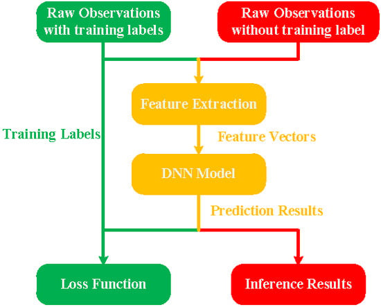
DNN is a category of machine learning algorithms implemented by stacking layers of neural networks with specific parameters. In RAIM-NET, the DNN is applied to classify the input feature as fault-alarm and fault-free for integrity monitoring. The framework of RAIM-NET consists of training and inference, as shown in Figure 1. The green blocks and lines belong to the training module, the red ones belong to the inference module, and the yellow ones belong to both. The raw observations with training labels and raw observations without training labels are input into the training module and inference module separately.
During training, the raw observations with training labels are used as input to the feature extraction block to calculate a feature vector. Then the feature vector is put into a DNN to obtain the prediction results, which is compared with the training labels in the loss function module. The parameters in the layers of the DNN model are then updated based on minimizing the loss function. As in most of the DNN model training procedures, the BP method is applied to train RAIM-NET by calculating the gradient of the loss function with respect to all the weights in the DNN model.
Inference comes after training, as it requires a converged neural network model. Unlike training, inference does not adjust the layers of the DNN model, but applies the knowledge from a trained DNN model and uses it to infer a result. During inference, the raw observations without the training label are used as input to the same feature extraction block to obtain the feature vector. Then the feature vector is input to the trained DNN model, which outputs the prediction results based on predictive accuracy of the DNN model. Finally, the inference results are output based on the probabilities of fault-alarm and fault-free in the prediction results.
2.2. Algorithm Description
2.2.1. Feature Extraction
Although the end-to-end DNNs that use the raw data as the input of the neural network are in fashion, the network architectures get more and more complex due to the lack of background knowledge for more challenging tasks [29]. For instance, without using the knowledge about the iterated least squares method [30], it might be very difficult to fit the GNSS positioning method using a stand-alone DNN model with raw data as the input. To meet the high performance requirements of integrity monitoring in real time and fault detection rate, the DNNs for RAIM should be easy to be trained and efficient for inference. To achieve this, feature extraction is specifically designed to make use of the background knowledge of RAIM. In our work, the feature vector is obtained in a similar way as the SS method, which is the difference between the full-set positioning solutions and the subset positioning solutions. Since the positioning difference of the feature vector is closely associated with the consistency checking in integrity monitoring, the features can be well related to the problem to be solved. In addition, the dimension of the feature vector is the number of the satellite observations, which is much less than the relative high dimension raw data including ephemeris observations and pseudoranges. The input dimension of DNN is significantly reduced and can be trained easily and efficient for inference.
Given an instance , the GNSS measurement formulation in East-North-Up (ENU) coordinate system can be described by the following equation [30],
where is the measurement vector, is the number of satellite observations, is the observation matrix, is the estimation vector in ENU coordinate system, which is composed of the three dimension position and receiver clock bias, is the observation error vector, which includes receiver noise, ionospheric delay error, multi-path error, etc. The term is the fault observation vector.
The measurement formulation of the subset observations can be obtained from Equation (1) as:
where is the matrix that can select the subset of the full observations, which is obtained from the identity matrix by deleting the row. The subscript is the excluded index number of the observation.
Through Equations (1) and (2), the positioning solution of the full observations and the positioning solutions of the subset observations are obtained using the iterated least squares method [30].
In this paper, the integrity in vertical coordinate is proposed as an example to investigate the RAIM-NET algorithm, which can also be easily extended to the integrity in the horizontal plane in our future work. Consider the vertical positioning result is determined by the third components of and [30], the feature vector used as an input for RAIM-NET is a simple concatenation of all the elements that relate to the vertical results, yields:
where is the extracted feature vector, are the vertical components of the difference positioning results in instance .
The extracted feature vector in parity space [12] is shown as an example in Figure 2. If the measurement vector in Equation (1) was noise-free and fault-free, the extracted feature vector in parity space would be the null vector. However, due to the combined effect of and , the feature vector in the parity space may land outside the detection boundary. In the existing snapshot algorithms, the fault observations are regarded as an independent event in each instance. Then, the fault-alarm is trigged only if the magnitude of the test statistic is larger than a threshold. However, in practice, the observations between each instance can be correlated, such as slowly increasing faults [18], which might cause a delayed alarm when using snapshot algorithms. Thus, if the intrinsic correlation of the time series feature can be extracted, the integrity monitoring challenges can be addressed in a timely manner.
2.2.2. DNN Model
To solve the problem of delaying fault-alarm when using the snapshot algorithms, the correlation in the extracted feature is researched to obtain an early fault detection result for integrity monitoring. Inspired by the RNNs in dealing with intrinsic correlation extraction in time series, LSTM, a typical case of RNN, is applied in RAIM-NET to regard the integrity monitoring solution as a classification problem with time series feature in this paper. Different from the snapshot algorithms that check whether the elements of the feature vector exceed a threshold or not under a statistical assumption, LSTM in RAIM-NET uses the training data to learn the distribution of the extracted features and for timely detection of fault observations.
Let be an input sequence of arbitrary length belonging to the set of all sequences over some input space. Let be the labels vector of the observation in each instance, where , 0 and 1 in the output space represent the fault-alarm and fault-free, respectively. The problem of integrity monitoring can be regarded as a method that can detect the fault as early as possible while the observation sequences continue appearing.
In this paper, multi-layer LSTM cells and a following Full Connected (FC) layer are stacked to obtain the DNN model for RAIM-NET; the total number of layers in our DNN model is denoted as . Each cell of the LSTM contains three gates serving as the controllers for information propagation within the network. The architecture of the vanilla LSTM with recurrent transition is given by [31], and the RAIM-NET is shown in Figure 3.
The hidden dimension of each layer of LSTM is the same, and the hidden unit of the layer is denoted as , where . There are four types of gates in each LSTM, i.e., input gate , update gate , output gate and forget gate . For each instance , the current input is denoted as , and then the working mechanism of LSTM is shown as:
where , , and are the weights matrix. The no-linear activation function is a sigmoid function.
The FC layer is a linear layer with an activation function following, i.e.,
where is the output of the last LSTM layer at instance , and are the weights matrix and bias vector, respectively. Then the output of the FC layer is input into a softmax function as:
where is the exponential function, is the index of the final output vector of the last layer of RAIM-NET . In Equation (6) and the elements of the output vector denote the probability of fault-alarm and fault-free for RAIM, respectively.
2.2.3. Loss Function
The parameters of the DNN model are trained using an optimization process that requires a loss function to calculate the model error. Then the DNN model is trained using stochastic gradient descent [32].
There are many loss functions to choose from. In this paper, the loss function is designed to directly respond to the accuracy rate of fault-alarm and fault-free of the prediction result of DNN model and the known labels of the training data. The cross entropy of the distribution of the prediction result relative to a distribution over a given training set is defined as follows:
where is the expectation function.
As the time sequence length of a training sample can be arbitrary, zero padding is used to align each mini batch with the maximum length for training. Denote as the batch size of each step in stochastic gradient descent, are the time sequence lengths of each training sample of the mini batch. Then, each sample of the mini batch is extended to length with zero padding. However, the part of the zero padding result should not be used to optimize the DNN model. Thus, combined with the discussion in the section of the DNN model, cross entropy can be obtained as:
By minimizing the loss function using stochastic gradient descent, we can obtain a DNN model that is used to classify fault-alarm and fault-free for fault detection tasks. However, to meet the stringent navigation requirement for integrity, a SS-based regularization is added to the loss function to integrate the advantages of the snapshot algorithm and temporal algorithm. The regularization is defined as a loss function where the test statistics exceeds the threshold of the SS method [12], i.e.,
where is the maximum value of the normalized test statistic vector; thus, we have:
where is the standard deviation. The threshold of SS method in Equation (9) can be obtained as:
where is the inverse tail probability distribution of the two-tailed standard normal distribution. , where is the standard normal cumulative distribution function. is the continuity risk requirement, parameter , and is the prior probability of fault-free occurrence.
Then, combined with Equations (8) and (9), the loss function with regularization for RAIM-NET can be obtained as:
where hyper-parameter is used to penalize the test statistics that exceed the threshold of the SS method. If , the loss function degenerated to the ordinary cross entropy. If , the RAIM-NET is to optimize the model parameters with the same performance of the SS algorithm.
2.3. Pseudocode for RAIM-NET
To present more specific details of our method, pseudocode for the training and inference of RAIM-NET is given in Algorithm 1 and Algorithm 2, respectively. The variables match the ones defined in Section 2.2.
The pseudocode for the RAIM-NET training is shown as follows:
| Algorithm 1: RAIM-NET Training | |
| Input: | |
| , training sample | |
| , measurement vector sequence | |
| , observation matrix sequence | |
| , labels sequence | |
| , arbitrary length of the sample | |
| , total number of samples in the training dataset | |
| , maximum number of visible satellites | |
| , nonlinear function of the DNN model in RAIM-NET with weights | |
| output: , converged model weights | |
| 1. initialize using a normal distribution with a mean of 0 and a standard deviation of 0.01 | |
| 2. while not converged do | |
| 3. sample minibatch of training samples from the dataset | |
| 4. for do | |
| 5. for do | |
| 6. obtain the number of visible satellites | |
| 7. calculate full positioning solution using Equation (1) | |
| 8. for do | |
| 9. calculate subset positioning solution using Equation (2) | |
| 10. end for | |
| 11. obtain using Equation (3) | |
| 12. pad the feature vector to dimension with zeros | |
| 13. concatenate feature vector to sequence | |
| 14. calculate the output of the DNN model using Equations (4)–(6) | |
| 15. end for | |
| 16. calculate the loss function using Equation (12) | |
| 17. end for | |
| 18. update the weights by descending its stochastic gradient with learning rate | |
| 19. end while | |
| 20. output the converged model weights | |
| The gradient-based updates can use any standard gradient-based learning rule. We used the Adam optimizer [33] in our experiments. | |
The pseudocode for the RAIM-NET inference is shown as follows:
| Algorithm 2: RAIM-NET Inference | |
| Input: | |
| , given an inference sample | |
| , measurement vector sequence | |
| , observation matrix sequence | |
| , arbitrary length of the sample | |
| , maximum number of visible satellites | |
| , nonlinear function of the DNN model with converged weights | |
| output: , prediction sequence | |
| 1. for do | |
| 2. obtain the number of visible satellites | |
| 3. calculate full positioning solution using Equation (1) | |
| 4. for do | |
| 5. calculate subset positioning solution using Equation (2) | |
| 6. end for | |
| 7. obtain using Equation (3) | |
| 8. pad the feature vector to dimension with zeros | |
| 9. concatenate feature vector to sequence | |
| 10. calculate the output of the DNN model using Equations (4)–(6) | |
| 11. if do | |
| , fault-alarm | |
| 12. else do | |
| , fault-free | |
| 13. end for | |
| 14. output the prediction sequence | |
3. Results
In this paper, real GNSS data is applied and two separated experiments are designed to evaluate the performance of RAIM-NET. The first experiment is to illustrate the property of RAIM-NET with different parameters, including the number of LSTM layers, hidden dimension of LSTM, and the hyper-parameter for regularization. The second experiment is to test the performance of RAIM-NET compared with the baseline RAIM methods of the GNSS receiver.
3.1. GNSS Data
GNSS data is designed to illustrate the performance of the proposed RAIM-NET. Considering that the real GNSS data with fault event is very difficult to obtain in practice, we add a manually fault event. In this paper, the real data was collected with a GNSS receiver (NovAtel DL-V3) in Beijing, China in January, 2019. The receiver was set to a fixed position with a 24-h average positioning of in an LLH (Longitude Latitude Height) coordinate system. The total amount of data for our experiments is samples of GNSS observations in 5Hz sampling rate, which was collected in about 56 h. Our experimental results show that RAIM-NET performs well on the dataset with the rate level. However, since RAIM-NET is proposed to detect faulty observation from the time series features, the data rate level is also an important factor for the detection results. Moreover, compared with the data collected at a static position, the feature sequence of the GNSS data in dynamic positions might be more complex. Although our proposed method performs well with static GNSS data, it might still face a challenge with dynamics inference due to the absence of dynamic data for training. The performance of RAIM-NET based on various datasets will be investigated in our future work.
The fault events are manually added to the observations of the real data. In this paper, two typical failure models are applied to illustrate the performance of RAIM-NET, i.e., step error and ramp error [18].
The failure model on the observation of step error is:
and the failure model on the observation of ramp error is:
where is the magnitude of the fault, is the unit step function and is the onset time of the failure, the slope of the fault is denoted as . The diagrams of the two failure modes are shown in Figure 4.
Iterating through all the real GNSS data in time series order, samples for RAIM-NET are constructed by selecting various real data series with random starting time and stopping time. The length of each sample obeys a uniform distribution from 5 to 50, i.e., . The samples with different length correspond to sequence observations from 1 s to 10 s in a 5 Hz rate level. As the time sequence samples for RAIM-NET are randomly constructed from the real observations, we can easily increase the amount of dataset with diverse random starting time and stopping time. In this paper, the total amount of data for RAIM-NET is . Then, half of these samples are selected randomly as the fault-free samples, and the other half is a manually added fault as the fault-alarm samples. The fault is randomly selected from the one mode of the step error and the ramp error and added to the real observations. In more detail, the onset time of the fault is randomly selected as . The magnitude of the step error obeys a uniform distribution from 0 m to 100 m, i.e., and the slope of the ramp error is randomly selected as , which makes the maximum magnitude of the ramp error obey . Specifically, in order to verify the detection rate and time delay decreasing of RAIM-NET, the maximum value of the fault we set needs to trigger the snapshot method, i.e., SS algorithm. Because too small faults may be ineffectively detected by any method, they are not included in the dataset. Finally, all of the data samples (fault or fault-free) are mixed together, and the dataset is randomly divided into a training set, validation set, and testing set with ratio of 8: 1: 1, which corresponds to , , and samples, respectively. With more real data, it would have been possible to increase the size of the testing set.
3.2. Results With Different Model Parameters
In the following experiments, the Adam optimizer [33] is used to train the weights of the LSTM model and the initial learning rate is , with an exponential decay at a rate proportional 0.9 for each epoch. The batch size is set to 64 for the following experiments.
3.2.1. Performance with Regularization
To test the performance of regularization in the loss function, training processes with different hyper-parameter are analyzed. The DNN model for this experiment is set to a five-layer LSTM with hidden dimension , and the accuracy detection rates for the validation set during the training processes with hyper-parameter from 0 to 1000 are plotted, as shown in Figure 5. Figure 5a,b are 1 minus detection rate and its logarithm during training processes, respectively. When , the loss function degenerates to the ordinary cross entropy without regularization. While the training process is convergent, the result is not stable in the validation. The reason might be that the DNN model is to be optimized with a global average performance on the training data, and does not specifically focus on individual samples that require fault-alarms. Considering that the integrity performance is very stringent for RAIM, the model checkpoint without regularization will be selected coincidently, causing unreliable performance for real applications. When , one can see that with a relatively large regularization, the model convergence is more stable but under fit. Due to the excessive regularization, the model tends to learn a representation to make its prediction results, focusing on the results of SS algorithm. It is not able to extract the knowledge of the sequence data, causing performance degradation. When or , the model convergence is stable with better fitting. Under the two different parameters, the detection rate of the convergence result in the validation set is larger than 99.9%. Therefore, the integrity performance is robust within this parameter range. As discussed above, this paper chooses as the final hyper-parameter for training.
3.2.2. Performance with Different LSTM Models
The number of model layers and the hidden dimension are two important indicators that affect the performance of the model. Table 1 shows the impact of different model layers on performance with the same hidden dimension . We compare different DNN models from 3 layers to 9 layers on the testing data. It is illustrated that as the number of model layers increases, model performance in detection rate for average alarm delay for ramp error gradually increases. However, the more the number of layers in the architecture, the slower the performance improvement.
The hidden dimension is another way to compare different model structures. Different model structures are designed with different number of layers and different hidden dimensions. To verify the effect of model depth and model width on the performance of integrity monitoring, the total number of model parameters is set to be the same. To achieve this, we increase the number of layers and reduce the hidden dimension, so that the number of parameters is kept close. As shown in Table 2, it can be seen that under the condition that the model parameters are about 1.75M, the performance of RAIM-NET is more benefited to the depth, when compared with the width of the DNN structure.
3.3. Results of Different RAIM Methods
As mentioned in [13], the SS and Chi-squared approaches are the two most widely implemented RAIM methods for fault detection. In order to test the practical application of RAIM-NET, two RAIM algorithms, i.e., SS algorithm and Chi-squared algorithm [13], are applied as the baseline methods to verify the performance improvement of RAIM-NET in terms of detection rate and alarm delay.
In this section, the DNN structure is set as five layers with hidden dimension . For the baseline methods, the detection threshold is set based on the Probability of False Alarms (PFA), which is the same with the continuity risk [13]. The detection rates of different methods for different fault magnitudes are counted. The performance of RAIM-NET on step errors and ramp errors are counted separately. Since the SS algorithm and Chi-squared algorithm can detect fault observation only if the magnitude is large enough to trig the alarm, the performance on the two different fault models is counted without distinction.
The fault detection rates of different methods are shown in Figure 6. When the fault magnitude is zero, the detection rates of the methods are PFAs. The PFAs of RAIM-NET, Chi-squared algorithm, SS algorithm are , , , respectively. The results show that our proposed method achieves the same probability of false alarm when compared with the baseline methods. The result also shows that the proposed RAIM-NET performs approximately for step errors and ramp errors, both of which are better than SS algorithm and Chi-squared algorithm with a higher fault detection rate under the conditions of the same fault magnitude. For example, when the fault bias is 30 m, the average fault detection rate for the two failure models of RAIM-NET is 97.2%, while the fault detection rates of SS algorithm and Chi-squared algorithm are 75.1% and 81.0%, respectively. RAIM-NET has a significant increase than the baseline methods in small fault detection. Taking into account that the detection power is 99%, the minimal detectable bias (MDB) [34] of the two baseline methods are 47 m and 45 m, while the proposed RAIM-NET obtains a smaller MDB as 33 m and 34 m for step errors and ramp errors, respectively. Conclusively, the proposed RAIM-NET outperforms the baseline methods with a higher level of fault detection rate and lower MDB in time series observations. By performing well in small fault detection, our experimental results show a potentiality of RAIM-NET obtaining smaller protection level to meet more stringent integrity requirements. However, unlike the SS algorithm that can obtain protection level easily, one of the disadvantages of RAIM-NET might be the inconvenience in protection level calculations.
Since the step error can only be detected by the SS algorithm or Chi-squared algorithm immediately when the magnitude is large enough to trig the alarm, we only used ramp error to test the alarm delay, as shown in Table 3. Our experimental results show that RAIM-NET can detect failure quicker than SS algorithm and Chi-squared algorithm, i.e., 51.8% and 48.2% relative average delay reduction on the testing set, respectively. Compared with the existing methods, our method can reduce delay time by about half. The standard deviation of the alarm delays with different methods is also calculated, as shown in Table 3. Considering three times of the standard deviation, i.e., 99.7% quantile, the alarm delays for SS algorithm, Chi-square algorithm, and RAIM-NET are 9.059s, 8.212s, and 5.610s, respectively. Although the proposed RAIM-NET is not trained to meet a specific application index, our method could be used as an important alternative if more timely alerts are required.
4. Conclusions
To ensure integrity, a navigation system is required to detect fault quickly and provide warnings to users. However, the standard RAIM method can only detect a fault that is instantly large enough to trig the alarm, which cannot meet more stringent applications. We propose a DNN-based RAIM, named RAIM-NET, to extract features of the fault in time series. Experimental results suggest that RAIM-NET can effectively detect small faults and provide an earlier fault-alarm than the SS algorithm and Chi-squared algorithm.
Dataset is an import factor for the performance of DNNs, including the proposed RAIM-NET. In our experiments, the real GNSS data for training is collected at a static position in 5 Hz sampling rate. For future developments, we propose to investigate the performance of RAIM-NET with different sampling rates and GNSS observations from dynamic positions. In addition, the DNN-based method for fault exclusion and other advanced solutions will be researched, e.g., attention mechanisms.
Funding
This research was funded by the National Natural Science Foundation of China grant number 61803037. And the APC was funded by the National Natural Science Foundation of China grant number 61803037.
Acknowledgments
The presented research work was supported by the National Natural Science Foundation of China (61803037).
Conflicts of Interest
The authors declare no conflict of interest.
References
- Hayath, M.T.; Begum, M.S. A Novel Review on Google Driverless Autonomous Vehicle. Int. J. Adv. Sci. Res. Eng. 2017, 3. [Google Scholar]
- Kong, S.-H.; Lopez-Salcedo, J.A.; Wu, Y.; Kim, E. IEEE Access Special Section Editorial: GNSS, Localization, and Navigation Technologies. IEEE Access 2019, 7, 131649–131652. [Google Scholar] [CrossRef]
- Cheng, N.; Lyu, F.; Chen, J.; Xu, W.; Haibo, Z.; Zhang, S.; Shen, X.S. Big Data Driven Vehicular Networks. IEEE Netw. 2018, 32, 160–167. [Google Scholar] [CrossRef] [Green Version]
- Sun, R.; Zhang, W.; Zheng, J.; Ochieng, W.Y. GNSS/INS Integration with Integrity Monitoring for UAV No-fly Zone Management. Remote Sens. 2020, 12, 524. [Google Scholar] [CrossRef] [Green Version]
- Angrisano, A.; Gaglione, S.; Crocetto, N.; Vultaggio, M. PANG-NAV: A tool for processing GNSS measurements in SPP, including RAIM functionality. GPS Solut. 2019, 24, 19. [Google Scholar] [CrossRef]
- Sun, Y.; Zhu, Y.; Xue, R. Multi-constellation Receiver Autonomous Integrity Monitoring with BDS/GPS/Galileo. In Proceedings of the Lecture Notes in Electrical Engineering; Springer Science and Business Media LLC; Springer: Berlin/Heidelberg, Germany, 2015; Volume 341, pp. 301–310. [Google Scholar]
- Yu, S.; Kim, D.; Song, J.; Kee, C. Covariance Analysis of Real-Time Precise GPS Orbit Estimated from Double-Differenced Carrier Phase Observations. Remote Sens. 2019, 11, 2271. [Google Scholar] [CrossRef] [Green Version]
- Bhattacharyya, S.; Gebre-Egziabher, D. Kalman filter–based RAIM for GNSS receivers. IEEE Trans. Aerosp. Electron. Syst. 2015, 51, 2444–2459. [Google Scholar] [CrossRef]
- Wang, E.; Jia, C.; Tong, G.; Qu, P.; Lan, X.; Pang, T. Fault detection and isolation in GPS receiver autonomous integrity monitoring based on chaos particle swarm optimization-particle filter algorithm. Adv. Space Res. 2018, 61, 1260–1272. [Google Scholar] [CrossRef]
- Yun, Y.; Yun, H.; Kim, D.; Kee, C. A Gaussian Sum Filter Approach for DGNSS Integrity Monitoring. J. Navig. 2008, 61, 687–703. [Google Scholar] [CrossRef]
- Brown, R.G. A Baseline GPS RAIM Scheme and a Note on the Equivalence of Three RAIM Methods. Navigation 1992, 39, 301–316. [Google Scholar] [CrossRef]
- Joerger, M.; Chan, F.-C.; Pervan, B. Solution Separation Versus Residual-Based RAIM. Navigation 2014, 61, 273–291. [Google Scholar] [CrossRef]
- Joerger, M.; Pervan, B. Fault detection and exclusion using solution separation and chi-squared ARAIM. IEEE Trans. Aerosp. Electron. Syst. 2016, 52, 726–742. [Google Scholar] [CrossRef]
- Sun, Y.; Zhang, J.; Xue, R. Leveraged fault identification method for receiver autonomous integrity monitoring. Chin. J. Aeronaut. 2015, 28, 1217–1225. [Google Scholar] [CrossRef] [Green Version]
- Jan, S.-S.; Gebre-Egziabher, D.; Walter, T.; Enge, P. Improving GPS-based landing system performance using an empirical barometric altimeter confidence bound. IEEE Trans. Aerosp. Electron. Syst. 2008, 44, 127–146. [Google Scholar] [CrossRef]
- Fu, L.; Zhang, J.; Li, R.; Cao, X.; Wang, J. Vision-Aided RAIM: A New Method for GPS Integrity Monitoring in Approach and Landing Phase. Sensors 2015, 15, 22854–22873. [Google Scholar] [CrossRef] [Green Version]
- Velaga, N.; Quddus, M.A.; Bristow, A.; Zheng, Y. Map-Aided Integrity Monitoring of a Land Vehicle Navigation System. IEEE Trans. Intell. Transp. Syst. 2012, 13, 848–858. [Google Scholar] [CrossRef]
- Bhatti, U.I.; Ochieng, W.Y.; Feng, S. Integrity of an Integrated GPS/INS System in the Presence of Slowly Growing Errors. Part I: A critical review. GPS Solut. 2007, 11, 173–181. [Google Scholar] [CrossRef]
- Federal Radionavigation Plan 2017; Department of Defense: Arlington, VA, USA; Department of Homeland Security: Arlington, VA, USA; Department of Transport: Arlington, VA, USA, 2017.
- Tran, T.H.; Presti, L.L. Kalman filter-based ARAIM algorithm for integrity monitoring in urban environment. ICT Express 2019, 5, 65–71. [Google Scholar] [CrossRef]
- Sun, Y.; Fu, L. A New Threat for Pseudorange-Based RAIM: Adversarial Attacks on GNSS Positioning. IEEE Access 2019, 7, 126051–126058. [Google Scholar] [CrossRef]
- Panagiotakopoulos, D.; Majumdar, A.; Ochieng, W.Y. Extreme value theory-based integrity monitoring of global navigation satellite systems. GPS Solut. 2013, 18, 133–145. [Google Scholar] [CrossRef] [Green Version]
- Peng, L.; Liu, P. Research on RAIM algorithm based on temporal filtering. In Proceedings of the 2014 IEEE International Conference on Control Science and Systems Engineering, Yantai, China, 29–30 December 2014; IEEE: New York, NY, USA, 2014; pp. 32–35. [Google Scholar]
- He, P.; Liu, G.; Tan, C.; Lu, Y.-E. Nonlinear fault detection threshold optimization method for RAIM algorithm using a heuristic approach. GPS Solut. 2015, 20, 863–875. [Google Scholar] [CrossRef]
- Wang, E.; Yang, F.; Tong, G.; Qu, P.; Pang, T. Particle Filtering Approach for GNSS RAIM and FPGA Implementation. Telkomnika 2016, 14. [Google Scholar] [CrossRef] [Green Version]
- Wang, E.; Pang, T.; Cai, M.; Zhang, Z. Application of Neural Network Aided Particle Filter in GPS Receiver Autonomous Integrity Monitoring. In Proceedings of the Lecture Notes in Electrical Engineering; Springer Science and Business Media LLC: Berlin/Heidelberg, Germany, 2014; Volume 304, pp. 147–157. [Google Scholar]
- Kim, D.; Cho, J. Improvement of Anomalous Behavior Detection of GNSS Signal Based on TDNN for Augmentation Systems. Sensors 2018, 18, 3800. [Google Scholar] [CrossRef] [PubMed] [Green Version]
- Hochreiter, S.; Schmidhuber, J. Long Short-Term Memory. Neural Comput. 1997, 9, 1735–1780. [Google Scholar] [CrossRef]
- Abdullah, T.; Bazi, Y.; Al Rahhal, M.M.; Mekhalfi, M.L.; Rangarajan, L.; Zuair, M. TextRS: Deep Bidirectional Triplet Network for Matching Text to Remote Sensing Images. Remote Sens. 2020, 12, 405. [Google Scholar] [CrossRef] [Green Version]
- Kaplan, E.; Hegarty, C. Understanding GPS: Principles and Applications, 2nd ed.; Artech House: Norwood, MA, USA, 2005. [Google Scholar]
- Zhao, H.; Sun, S.; Jin, B. Sequential Fault Diagnosis Based on LSTM Neural Network. IEEE Access. 2018, 6, 12929–12939. [Google Scholar] [CrossRef]
- Bottou, L. Large-Scale Machine Learning with Stochastic Gradient Descent. In Proceedings of COMPSTAT’2010; Springer Science and Business Media LLC, Physcica-Verlag HD: Berlin/Heidelberg, Germany, 2010; pp. 177–186. [Google Scholar]
- Kingma, D.P.; Ba, J. Adam: A Method for Stochastic Optimization. arXiv 2014, arXiv:1412.6980. [Google Scholar]
- Milner, C.; Ochieng, W.Y. Weighted RAIM for APV: The Ideal Protection Level. J. Navig. 2010, 64, 61–73. [Google Scholar] [CrossRef]
Figure 1.
The framework of the proposed RAIM-NET.

Figure 2.
The extracted feature vector series in the parity space.

Figure 3.
The architecture of the DNN model.

Figure 4.
The diagrams of the step error and the ramp error. (a) Step error; (b) Ramp error.

Figure 5.
The training processes with different regularization. (a) (1—detection rate) during training processes; (b) log10(1—detection rate) during training processes.
Figure 5.
The training processes with different regularization. (a) (1—detection rate) during training processes; (b) log10(1—detection rate) during training processes.


Figure 6.
Fault detection rates of different methods.


Table 1.
Performance with different model layers.
| Layers | Detection Rate | Alarm Delay |
|---|---|---|
| 3 | 99.776% | 1.345 s |
| 5 | 99.903% | 1.137 s |
| 7 | 99.923% | 1.109 s |
| 9 | 99.925% | 1.110 s |
Table 2.
Performance with different hidden dimensions.
| Layers | 3 | 5 | 7 |
|---|---|---|---|
| Hidden Dimension | 172 | 128 | 106 |
| Number of Parameters | 1.73 M | 1.75 M | 1.74 M |
| Detection Rate | 99.819% | 99.903% | 99.918% |
| Alarm Delay | 1.285 s | 1.137s | 1.128 s |
Table 3.
Alarm delay of RAIM-NET and other methods for ramp error.
| Methods | Alarm Delay | |
|---|---|---|
| Mean | Standard Deviation | |
| SS algorithm | 2.840 s | 2.073 s |
| Chi-square algorithm | 2.641 s | 1.857 s |
| RAIM-NET | 1.368 s | 1.414 s |
© 2020 by the author. Licensee MDPI, Basel, Switzerland. This article is an open access article distributed under the terms and conditions of the Creative Commons Attribution (CC BY) license (http://creativecommons.org/licenses/by/4.0/).
Share and Cite
MDPI and ACS Style
Sun, Y. RAIM-NET: A Deep Neural Network for Receiver Autonomous Integrity Monitoring. Remote Sens. 2020, 12, 1503. https://doi.org/10.3390/rs12091503
AMA Style
Sun Y. RAIM-NET: A Deep Neural Network for Receiver Autonomous Integrity Monitoring. Remote Sensing. 2020; 12(9):1503. https://doi.org/10.3390/rs12091503
Chicago/Turabian StyleSun, Yuan. 2020. "RAIM-NET: A Deep Neural Network for Receiver Autonomous Integrity Monitoring" Remote Sensing 12, no. 9: 1503. https://doi.org/10.3390/rs12091503
Note that from the first issue of 2016, this journal uses article numbers instead of page numbers. See further details here.