1. Introduction
In rivers and streams where humans have altered the thermal regime, not only does summer water temperature frequently exceed the thermal tolerance of native salmonids, thus influencing their distribution [
1], but these human modifications can amplify or dampen spatial and temporal variation [
2]. Specifically, dams and diversions can greatly modify riverine thermal regimes by restricting or eliminating connectivity in longitudinal, lateral, vertical, and temporal dimensions [
3,
4]. Large dams can be intentionally managed to release cold water from deep reservoirs to provide habitat for salmonid fisheries, whereas releases from any size dam and diversion can increase downstream temperatures by releasing warm water directly from the reservoir surface [
5].
The thermal effects of dams have been studied for many years [
6,
7], and it is recognized that these effects depend on the landscape position of the dam, dam operation, water release depth, and geomorphic setting [
5]. Direct modifications to the thermal regime are made by upstream water releases and dam operations. When taking into consideration the geomorphic setting, confined valleys are likely to be more susceptible to changes in water temperature due to water releases than are unconfined valleys, which have greater surface water-groundwater exchange and greater hydrologic storage [
8]. Indirect modifications of the thermal regime are those that affect the processes of heat exchange between water and the environment [
9]. These indirect modifications to the thermal regime occur when dams alter sediment transport and channel geometry and fragment riparian and riverine habitat [
8,
10,
11,
12]. In impounded rivers, flow velocity, water depth, and the extent of channel wetted perimeter are decoupled (spatially and temporally) from the river’s geomorphic setting due to dam operations [
8]. Water releases from the dam that have a limited sediment load and excess energy may incise the channel bed and coarsen the channel bed material [
11]. However, dam effects on flow and sediment are also dependent on the geomorphic setting where lateral and vertical movement of flow and sediment are constrained by valley shape [
8]. Changes in water depth and flow velocity are likely greatest in confined valleys, whereas changes in the extent of wetted perimeter and channel width may be largest in unconfined valleys, such as in the Colorado, Green, and Missouri rivers [
8,
13].
The mechanisms by which channel geometry (i.e., water depth, wetted perimeter, stream width, and cross-sectional area) indirectly affect water temperature are complex. In confined sections of a river where the river is narrow and deep, two main mechanisms may be at play, depending on flow velocity. At high flow velocities, water may be cooler due to mixing and topographic shading, but at low velocities, thermal stratification may occur in the summer when surface water temperature is higher than deeper water. In contrast, in unconfined sections, where changes in wetted perimeter and channel width are largest, warmer water temperatures are the result of a larger surface area exposed to solar radiation [
14]. Rivers with dense submerged aquatic vegetation (SAV) may also experience thermal stratification, as SAV steepens vertical temperature gradients and decreases water velocity [
15].
Tributaries and groundwater inputs can also have an impact on the thermal regime and its variability by creating discontinuities in the longitudinal profile regardless of whether a river or stream is dammed or not [
16,
17,
18]. The extent of the influence of these tributaries and groundwater inputs on the physical characteristics of the main stem river depend on their size relative to the main stem, morphology or junction angle, and dam operations [
8,
19,
20,
21,
22,
23,
24].
Although dam-induced modifications to a river’s thermal regime can influence the quantity and distribution of cold-water refuges for salmonids, cold-water refuge quantity and distribution in large impounded rivers have not been well studied. Previous studies on the spatial and temporal variability of water temperature and cold-water refuges have focused on small- to medium-size streams [
16,
25,
26,
27,
28,
29] and some large unregulated rivers [
18,
30,
31]. In contrast, studies on large regulated rivers have mostly emphasized thermal variability changes [
8,
32,
33,
34] or their cold-water refuge distribution [
35,
36,
37], but not both.
In the Pend Oreille River, adult bull trout (
Salvelinus confluentus) and westslope cutthroat trout (
Oncorhynchus clarkii lewisi) experience summer water temperatures that exceed their upper tolerances, 18–20 °C [
38,
39,
40,
41,
42]. Bull trout and westslope cutthroat trout in Pend Oreille River telemetry studies have been observed behaviorally thermoregulating in cold tributary confluences and areas with groundwater inputs (E.K. Berntsen, J.R. Maroney, and J. Connor, Kalispel Tribe of Indians, personal observation). We examined thermal heterogeneity across space and time and identified potential cold-water refuges for adult salmonids in the Pend Oreille River, a large impounded river with an epilimnetic-release dam in the inland northwestern USA. We had three specific objectives:
- (1)
Compare longitudinal patterns of water temperature derived from thermal infrared imagery to instream measurements in the water column.
- (2)
Assess spatial (lateral, longitudinal, and vertical) and temporal thermal heterogeneity and potential cold-water refuges for salmonids at multiple scales.
- (3)
Evaluate statistical associations between hydrologic and geomorphic variables and occurrence of cool-water areas and median water temperature.
We hypothesized that (1) water temperature in the main stem of the Pend Oreille River increases as water moves downstream, but lateral contributions from tributaries create discontinuities in the longitudinal profile; (2) the confluence area formed by the main stem Pend Oreille River and cold tributaries provide potential cold-water refuges for cold-water fishes; and (3) in the summer, thermal stratification from various sources (i.e., seeps, groundwater inputs, low water velocities, and submerged aquatic vegetation) creates vertical temperature gradients that isolate cool water near the river bottom to potentially provide refuge for fish.
4. Discussion
We combined the high spatial resolution of airborne thermal infrared (TIR) imagery with the high temporal resolution of instream measurements to describe broad-scale patterns of water temperature in relation to localized drivers of heterogeneity. Our findings demonstrated that (1) lateral contributions from tributaries along the longitudinal profile dominated thermal heterogeneity in the Pend Oreille River, (2) spatial and temporal thermal variability at confluences was approximately an order of magnitude greater than that of the main stem, (3) most of the potential cold-water refuges were found at confluences regardless of the refuge definition used, and (4) the probability of occurrence of cool areas and the median radiant water temperature were closely linked to geomorphic metrics at the reach scale and to the distance from the Albeni Falls Dam at the subcatchment scale. These results highlight the importance of using multiple approaches to describe thermal heterogeneity in large impounded rivers. TIR data alone provided an incomplete picture of the thermal variability found at tributary confluences and in areas of the main stem with vertical stratification. Instream thermographs at the bottom of most confluences recorded considerably cooler temperatures than surface loggers and revealed discontinuities in the longitudinal profile that were not observed in the TIR data. These results have important implications for the identification and restoration of cold-water refuges.
This study also expands understanding of thermal heterogeneity in large impounded rivers by complementing earlier work, mostly in Europe and North America (e.g., [
8,
32,
33]). Overall, we observed a slight downstream increase in water temperature along the longitudinal profile with multiple peaks and troughs. A downstream increase in water temperature is a pattern that has been reported in many rivers and, until recently, was our conceptual model for rivers in general [
26]. Like Arscott et al. [
30], we found that lateral heterogeneity dominated thermal heterogeneity. Lateral heterogeneity in our study was an order of magnitude greater than longitudinal heterogeneity, but unlike Arscott et al. [
30] where this variability was related to floodplain habitat, lateral variability in our study is associated with tributary confluences, as most floodplain habitat has been modified in the Pend Oreille River. Other studies [
67,
68,
69] have investigated lateral heterogeneity at the segment and reach scales but longitudinal heterogeneity was not considered.
Because the rivers surveyed with TIR remote sensing are generally well mixed vertically except at isolated large features such as pools [
16,
26], previous studies have focused mostly on thermal variability in longitudinal and lateral dimensions [
26,
67,
68]. Persistent thermal stratification in main river channels seldom occurs because streamflow is usually turbulent enough to cause complete mixing [
70]. Like previous studies on riverine thermal stratification, we found that stratification in the main stem was only persistent at one site, P4, where the river was shallow, slow moving, unconfined, and had dense patches of aquatic vegetation. However, it is important to consider temporal variability of vertical thermal gradients because of their potential use by fish as ambient cold-water refuges. We found that 10 main stem sites had differences between surface and bottom water greater than 1 °C for at least one hour per day about 50% of the time. This difference appears small, but it may provide salmonids thermal refuge during migration while fish travel to and from cold-water refuges that better meet their physiological needs.
Our results corroborate those of Wawrzyniak et al. [
71] who found that TIR-derived temperatures overestimated in situ measurements at most confluences where thermal stratification was regularly observed. In addition, four confluences were stratified persistently, near 100% of the time (C1, C3, C4, and C5), two confluences were hardly ever stratified (C2, C13), and the rest of the confluences were stratified between 13 and 87% of the time. In a tributary of Three Gorges Reservoir in China, Jin et al. [
72] found that the main drivers of stratification were reservoir operations (i.e., water level and water fluctuations) and air temperature which were not included in our study but are likely important factors in our study. We also speculate that temperature of the incoming tributary, volume of water, and water velocity at the confluences are important drivers influencing thermal stratification because the four confluences where we observed persistent stratification (95–100%) had low water velocity and temperature differences of at least 4 °C at the bottoms of the incoming tributary and the main stem.
These findings illustrate that the identification of a potential cold-water refuge depends on the definition used (i.e., the criteria) and the temporal scale observed. For instance, we did not observe main stem water temperatures cooler than 18 °C during our study; therefore, no main stem sites were classified as potential physiological cold-water refuges. However, when we assessed the main stem sites using our least restrictive 1 °C ambient criterion, all sites were considered cold-water refuges at depth during some portion of the day, albeit over different periods of time. Consequently, cold-water refuge definitions based solely on physiological thresholds or that exclude fine temporal and spatial scales overlook the importance of thermal heterogeneity for providing thermal refuge when temperatures exceed physiological thresholds even if it is for few hours a day [
55]. Because most studies have focused on the spatial variability of cold-water refuges [
1,
16,
45,
59], cold-water refuge persistence has not been well studied. Dugdale et al. [
18] documented in the Miramichi River that 61% of thermal refuges (≥0.5 °C colder than the ambient river channel temperature) were only identified once during multiple TIR surveys. In our study, we found that the persistence of confluence cold-water refuges was associated with the difference in 7DADM for the main stem and the confluence; larger differences in temperature created refuges that were persistent over longer periods, regardless of how refuges were defined.
We designed our study to describe water temperature patterns in the Pend Oreille River when conditions were warmest to understand how thermal heterogeneity during these stressful conditions influence cold-water refuge distribution for salmonids. Because water temperature was already above 20 °C when we started sampling in 2017, and water temperature in the main stem Pend Oreille River reached 18 °C during the first week of July [
73], bull trout and, to a lesser extent, cutthroat trout were under thermal stress for most of the summer. Thus, using physiological thresholds alone for the main stem Pend Oreille was not very informative. However, comparing the spacing of cold-water refuges together with their persistence can help evaluate whether these refuges are adequate for salmonids migrating through the Pend Oreille River. Spacing along the longitudinal profile between persistent cold-water refuges (i.e., those that were present 100% of the time) that are formed by confluences ranged between 2 and 41 km (median = 7 km), but when we considered physiological cold-water refuges that were present at least 50% of the time, the spacing was reduced to less than 18 km, with an increase in the median separation distance (11 km). Additionally, areas that are 1–2 °C cooler than the median main stem bottom water temperature (main stem ambient cold-water refuges) but are still above the physiological thresholds can provide connectivity and can be used as stepping stones during migration [
59]. Spatially continuous bottom water temperatures would be needed to determine the spacing of ambient cold-water refuges in the main stem along the longitudinal profile. Furthermore, we did not include every confluence in our analysis, so our numbers for cold-water refuge spacing are most likely overestimated, especially if localized groundwater inputs occur at depth or are too small to be detected at the surface using remotely sensed methods (e.g., TIR). Nevertheless, our spacing estimates for the confluences were within the range of variation of previous studies. Fullerton et al. [
59], in a review of rivers in the Pacific Northwest, reported two to three times the median spacing of this study, but the spacing had high variability and ranged from 6 to 49 km, whereas Dzara et al. [
28] in the Walker River in Nevada found that median spacing was 0.9 km and ranged from 0.3 to 37 km.
The high resolution of the geomorphic metrics measured along most of the Pend Oreille River provides a unique opportunity to examine how these metrics affect the occurrence of cool areas and median water temperature at the 1-km scale. The strong associations with channel confinement corroborated findings of previous studies [
17,
22,
30,
74]. Cross-sectional area, another variable with strong explanatory power for both reach-scale models, was also inversely correlated with water column velocity (Pearson correlation = −0.90). These robust associations support our hypotheses that channel confinement, water velocity, and cross-sectional areas explain different mechanisms that directly affect water temperature patterns. More specifically, at confined sections where the river is narrow and deeper, two alternative mechanisms may be at play depending on water velocity. At high velocities, water may be cooler as a result of mixing of the water column and topographic shading, whereas at low velocities, water may be warmer at the surface due to thermal stratification. In contrast, at unconfined sections, where channel width and cross-sectional area are largest, warmer water temperatures are the result of greater surface area being exposed to solar radiation.
At the subcatchment scale, our models suggest that the distance from Albeni Falls Dam was the most important factor determining the occurrence of cool water areas and explaining median water temperature. This result was unexpected for our study because of the weak longitudinal downstream patterns observed in the TIR data. However, our statistical results corresponded to those found in other studies when location in the network was considered [
74,
75]. The mechanism for this downstream increase was not entirely clear from our results. A regional study of the impact of dams on water temperature in Eastern Canada found that dams with impounded runoff index (storage capacity divided by median annual runoff) less than 10% had little impact on the thermal regime of medium-size rivers [
76]. The Pend Oreille River is at least an order of magnitude larger than the rivers described by Maheu et al. [
27], and has an impounded runoff index of less than 1%, which is typical of run-of-the-river systems. However, during most of the 2001 summer when the TIR data were collected, assuming no major withdrawals, the reservoir was storing water. The amount of time that the daily reservoir outflow was less than daily reservoir inflow was 82% in July, 70% in August, and 13% in September. The largest daily difference between outflow and inflow was 18% on August 7. Despite the Pend Oreille River having run-of-the-river characteristics on an annual basis, the reservoir appears to operate as a storage reservoir in the summer and is likely to experience a warming effect. Our statistical results did not point to the size or number of tributaries as explanatory variables. These results, together with TIR imagery from tributary plumes suggest that lateral contributions were operating at the reach scale, except at the lowest trough (rkm 80 to 90), where C6 and C5 were large enough to potentially have an impact on downstream water temperature patterns.
We recognize that our TIR survey was conducted in 2001 and our instream thermographs were deployed in 2017. Although, this mismatch could influence our interpretations, Fullerton et al. [
26] found that spatial patterns of water temperature from repeat TIR surveys were consistent among years and, thus, comparisons with broad spatial patterns data collected in 2017 should be consistent over time given that the river morphology has not changed. Similarly, 3-D mapping was conducted at considerably different discharges: Average discharge from the second survey was almost three times the discharge from the first survey (268 m
3 s
−1 versus 720 m
3 s
−1). We used z-scores to normalize these values to account for the temporal variability. The z-scores directly compare the patterns of variability rather than the magnitude of the variables and can be used as explanatory variables by removing any bias potential from sampling during different flow conditions. We also recognized that some confluences were highly spatially variable due to either their low stream bed stability (substrates were mostly sand or silt) or their dense aquatic vegetation, so placement directly below the thermal plume and foreseeing the path of the tributary was not possible. For these types of streams (e.g., C14, C8, C7, and C17), distributed temperature sensing (DTS) cables could have captured the plume path more consistently than instream loggers as the water elevation decreased. However, budget constraints and potential logistical and maintenance issues prevented our use of DTS. Incorporating this variability can be informative to management for potential cold-water refuges at these confluences with fluctuating conditions. Finally, our study was limited to one large, impounded river with specific geomorphic and hydrologic characteristics and flow operations. However, inferences from this study may still be relevant to other run-of-the-river reservoirs with similar physical characteristics.
Many questions remain about the thermal heterogeneity of large impounded rivers, and the implications for cold-water refuges. Because thermal heterogeneity is likely dampened in the main stem river, studies that consider flow management scenarios affecting the size, spacing, and persistence of cold-water refuges may be critical to develop management strategies for conserving, augmenting, and restoring areas suitable for salmonids. Our study also raises questions about the sufficiency of the potential cold-water refuges described here. Understanding the adequacy of cold-water refuges for bull trout and cutthroat trout migration is important for the survival of these species in the Pend Oreille River system. Suitability of cold-water refuges is not limited to water temperature; therefore, other factors such as dissolved oxygen and food availability should also be considered when determining the potential use of a cold-water refuge. For instance, we observed bull trout at C3 and C17 where dense abundant vegetation and night hypoxic conditions were present. Dense SAV may negatively impact these areas by decreasing dissolved oxygen at night near the bottom where it is cooler and may prevent fish from using these areas if SAV becomes so thick that it creates a barrier. Understanding the interactions between submerged aquatic vegetation, water temperature, and dissolved oxygen may provide management strategies at confluences where these conditions occur. Lastly, our findings suggest that the distance from Albeni Falls Dam was an important variable explaining occurrence of cool areas and median water temperature. Hence, understanding statistical associations of hydroclimatic variables related to conditions upstream of the dam, such as upstream water temperature, discharge, ratio of reservoir outflow to inflow, and air temperature to downstream water temperature could be used to examine whether Albeni Falls Dam affects downstream water temperature patterns.
Given that climate change will increase temperatures globally, thermal heterogeneity will become increasingly important for fish to behaviorally thermoregulate during times of thermal stress even as the ability of fish to locate cold-water areas is also diminished because of habitat homogenization [
77]. Because unidentified refuges are at risk of being lost through habitat modification and degradation or unsuitable management [
78], locating cold-water refuges is the first step to manage, restore, augment, and create thermal heterogeneity to conserve salmonid habitat [
79].

 and
and 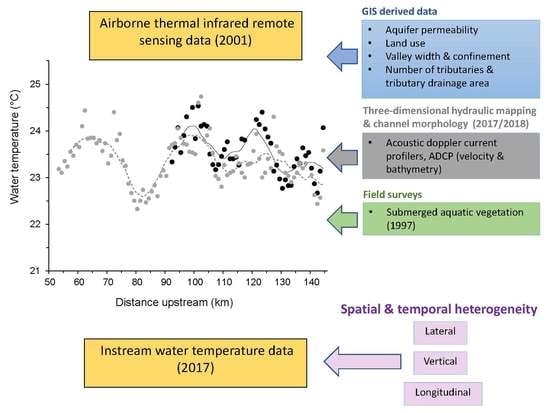


