Article

Monitoring Invasion Process of Spartina alterniflora by Seasonal Sentinel-2 Imagery and an Object-Based Random Forest Classification

1
Key Laboratory of Wetland Ecology and Environment, Northeast Institute of Geography and Agroecology, Chinese Academy of Sciences, Changchun 130102, China
2
University of Chinese Academy of Sciences, Beijing 100049, China
3
National Earth System Science Data Center of China, Beijing 100101, China
4
State Key Laboratory of Information Engineering in Surveying, Mapping and Remote Sensing, Wuhan University, Wuhan 430079, China
*
Author to whom correspondence should be addressed.
Remote Sens. 2020, 12(9), 1383; https://doi.org/10.3390/rs12091383
Submission received: 27 March 2020 / Revised: 24 April 2020 / Accepted: 26 April 2020 / Published: 27 April 2020
(This article belongs to the Special Issue Remote Sensing of Wetlands)

Abstract

:
In the late 1990s, the exotic plant Spartina alterniflora (S. alterniflora), was introduced to the Zhangjiang Estuary of China for tidal zone reclamation and protection. However, it invaded rapidly and has caused serious ecological problems. Accurate information on the seasonal invasion of S. alterniflora is vital to understand invasion pattern and mechanism, especially at a high temporal resolution. This study aimed to explore the S. alterniflora invasion process at a seasonal scale from 2016 to 2018. However, due to the uncertainties caused by periodic inundation of local tides, accurately monitoring the spatial extent of S. alterniflora is challenging. Thus, to achieve the goal and address the challenge, we firstly built a high-quality seasonal Sentinel-2 image collection by developing a new submerged S. alterniflora index (SAI) to reduce the errors caused by high tide fluctuations. Then, an object-based random forest (RF) classification method was applied to the image collection. Finally, seasonal extents of S. alterniflora were captured. Results showed that (1) the red edge bands (bands 5, 6, and 7) of Sentinel-2 imagery played critical roles in delineating submerged S. alterniflora; (2) during March 2016 to November 2018, the extent of S. alterniflora increased from 151.7 to 270.3 ha, with an annual invasion rate of 39.5 ha; (3) S. alterniflora invaded with a rate of 31.5 ha/season during growing season and 12.1 ha/season during dormant season. To our knowledge, this is the first study monitoring S. alterniflora invasion process at a seasonal scale during continuous years, discovering that S. alterniflora also expands during dormant seasons. This discovery is of great significance for understanding the invasion pattern and mechanism of S. alterniflora and will facilitate coastal biodiversity conservation efforts.

Graphical Abstract

1. Introduction

Spartina alterniflora (S. alterniflora) was introduced to China from North America in 1979 for the purpose of stabilizing seashore, reclaiming tidal land, and improving soil quality [1]. However, during the past three decades, S. alterniflora has been aggressively invading native coastal vegetation with an invasion rate of 137 km2 per decade [2]. According to recent studies, S. alterniflora posed a great threat to many native communities and coastal environments by competing with native plants, altering feeding habitats of shorebirds in open mudflats, and transforming characteristics of native species [3,4,5]. With increasing awareness of the negative impacts of S. alterniflora, local and central governments are paying close attention to managing S. alterniflora invasion. Comprehensive management relies on detailed continuous information of S. alterniflora distributions, especially at a high temporal resolution [6]. However, obtaining such information is a great challenge due to the high spatiotemporal variation of S. alterniflora in complex coastal environments [1].
Remote sensing has been shown as a viable tool in monitoring dynamics of invasive plants [7]. Landsat imagery with moderate spatial resolution (30 m) has been widely used in mapping S. alterniflora invasions [7,8,9]. However, due to Landsat’s spatial resolution, spatial details of newly colonized S. alterniflora patches were usually omitted. In the past two decades, high-resolution satellite images, such as those of WorldView-2/3, SPOT-5/6, and Gaofen-1/2, have been used to monitor S. alterniflora changes [4,6,10,11]. However, all these images are commercial products, which are costly and make it difficult to guarantee long-term regular observations [12,13]. In recent years, Sentinel-2, which gives continuity to the multispectral fine-resolution optical observations, has received more and more attention in vegetation monitoring [14,15]. With Sentinel-2, it is possible to capture a detailed spatiotemporal process of a vegetation community, because it carries a state-of-the-art sensor of 13 spectral bands and a 2–5 day re-entry cycle [16]. The visible and near-infrared (NIR) bands have finer spatial resolution (10 m) than other medium-resolution satellite images. In addition, compared to commonly used high-resolution satellite images, such as WordView-2/3, SPOT-5/6, and Gaofen-1/2, Sentinel-2 has more detailed spectral information (three red edge bands and 1 narrow NIR band). These bands are essential to increase the capability of vegetation detection. Accordingly, Magnus Persson et al. found the classification accuracy of common species over a mature forest was improved by using Sentinel-2 imagery in central Sweden [17]. Grabska et al. showed that the use of the Sentinel-2 time series instead of single date imagery significantly improved forest tree species mapping by approximately 5%–10% of overall accuracy [18]. Furthermore, David et al. (2017) highlighted that wavelength regions in red edge bands, narrow NIR, and short-wave infrared reflectance (SWIR) are characterized by a sharp increase in vegetation reflectance, while water shows strong absorption in these spectral ranges [19]. Wang et al. (2018) and Jia et al. (2019) suggested using these spectral bands and derived indices in Sentinel-2 imagery for accurately mapping the extent of coastal and aquatic vegetation [20,21]. Their results showed that the freely accessed 10 m spatial resolution Sentinel-2 imagery has made it possible to implement robust and efficient monitoring of S. alterniflora invasions.
For years, various remote-sensing-based methodologies have been employed to monitor the extents of S. alterniflora [2,11,22,23,24]. Recently, machine learning algorithms, including support vector machines (SVM), random forest (RF), and K-nearest neighbor (KNN), have been used to map S. alterniflora [25,26,27,28]. However, most of these studies were conducted with pixel-based classification method; spatial characteristics, such as shape and texture, which are important to improve classification accuracy, were not applied to identify S. alterniflora. In contrast, the object-based image analysis (OBIA) fully considers texture, shape, and geometric features, so that more accurate and robust results are obtained than those of pixel-based method [29,30,31]. The OBIA can effectively address the “salt-and-pepper” effect and reduce within-class spectral variation. Therefore, in recent years, more and more studies have introduced OBIA and machine learning algorithms to delineate S. alterniflora [2]. For example, SVM is based on the principle of support vector classifier, a linear classifier. It was developed by using different kernel functions to solve nonlinear problems, which also leads to the training process of SVM usually being more time-consuming [32]. In contrast, RF algorithm has unique advantages in remote sensing classification. As a kind of ensemble learning classification algorithm, RF algorithm not only addresses the problem of overfitting found in previous machine learning algorithms such as SVM, but also can be successfully used to select and rank the variables with the greatest ability to discriminate between the target classes [33]. In remote sensing image classification, the use of RF algorithm has received increasing attention due to the excellent classification results obtained and the speed of processing [26,27,34]. The combined method has greatly contributed to monitoring invasion processes of S. alterniflora [4].
Although there have been studies in the past to monitor the distribution of S. alterniflora, results that contain accurate and timely interpretation of these relatively small patches have been rare, due to the lack of full consideration of tidal conditions [35,36,37]. S. alterniflora are periodically submerged by the rising tides, especially in regions with high tidal fluctuations and newly colonized lower S. alterniflora patches [37,38], as this species is found in near-shore zones. Ideally, it is better to use images acquired during low tides; however, such data are difficult to obtain due to the uncertainties of local instantaneous tidal conditions during the predetermined times that satellites pass over. Unlike terrestrial ecosystems, S. alterniflora is difficult to monitor because of the uncertainties caused by periodic inundation of local tides, especially in regions with high tide fluctuations [39,40]. Thus, the aims of this study are to (1) remove the influence of tidal fluctuations to build a high-quality seasonal Sentinel-2 image collection; (2) accurately map seasonal status and distributions of S. alterniflora by Sentinel-2 images and combined method (machine learning algorithm and OBIA); (3) analyze S. alterniflora invasions at a seasonal scale. This study aims to identify the advantages and potential of Sentinel-2 imagery in mapping of S. alterniflora and provide a more effective monitoring method for intertidal vegetation changes. The seasonal invasion process of S. alterniflora detailed by this study will provide a new perspective for ecologists and environmental managers to understand the invasion mechanism of S. alterniflora.

2. Materials and Methods

2.1. Study Area

The study area is the core zone of Fujian Zhangjiang Estuary Mangrove National Nature Reserve, which has an area of 2.5 km2 and is located in the estuary of Zhangjiang River, Yunxiao County, Fujian Province, China (117°24′07″–117°30′00″E, 23°53′45″–23°56′00″N; Figure 1). This reserve was listed as a national nature reserve in 2002 and added to the Wetlands of International Importance (Ramsar site No. 1726) in 2008. Zhangjiang Estuary has a semidiurnal tide type with 0.43 m minimal tidal range, 4.67 m maximal tidal range, and 2.32 m annual mean tidal variation. The region has a monsoon-influenced marine subtropical climate, with temperature varying from 0.2 to 38.1 °C and precipitation varying from 1348 to 2493 mm. The study area is characterized by native species of Avicennia marina, Aegiceras corniculatum, and Kandelia obovate. S. alterniflora has been invading this region since the early 1990s, now, it is a common species with the largest area in the reserve [41].
According to the phenological characteristics of S. alterniflora, we divided each year into the two seasons of growing season and dormant season [42]. The growing season is from March to October, and the residual months (November–February) are defined as the dormant season [43].

2.2. Sentinel-2 Imagery and Ground References

Cloud-free Sentinel-2 imagery was downloaded from the website of Copernicus Sentinels Scientific Data Hub (https://scihub.copernicus.eu/) and was delivered orthorectified with top-of-atmosphere reflectance in Universal Transverse Mercator (UTM) projection with the World Geodetic System (WGS 84). The Sentinel-2 mission is comprised of two satellites, Sentinel-2A and Sentinel-2B. Both carry a state-of-the-art MultiSpectral Instrument (MSI) sensor which offers 13 spectral bands, spanning from the visible, through the NIR and red edge, to the SWIR. They have great potential for various applications of earth observation [44]. Bands acquired at 60 m (coastal aerosol band 1, water vapor band 9 and cirrus band 10) spatial resolution are dedicated primarily for detecting atmospheric features and were therefore excluded from the analysis [16]. Table 1 lists the general characteristics of the Sentinal-2 imagery.
To monitor seasonal invasion process of S. alterniflora, we downloaded cloud-free level 1C (radiometric and geometric corrections) Sentinel-2 images from the beginning of growing seasons (February 2016, March 2017, March 2018) and the dormant seasons (December 2016, November 2017, November 2018) over Zhangjiang Estuary from 2016 to 2018. Detailed information and tidal levels of these images are presented in Table 2. Geometric and radiometric corrections with subpixel accuracy, such as spatial and orthorectification registration on a global reference system, were made by the Level-1C product. In the toolbox of Sentinel Application Platform (SNAP), the atmospheric correction (converting top-of-atmosphere reflectance into top-of-canopy reflectance) of the Sentinel-2 image was performed using the atmospheric correction tool of SEN2COR (version 2.05.05). After atmospheric correction, bands with 60 m spatial resolution (Bands 1, 9, 10) were abandoned. All other bands had a resampled pixel size of 10 m × 10 m to standardize different spatial resolutions of bands in Sentinel-2 images.
Ground surveys were conducted in November 2016, November 2017, and November 2018. The location of each sampling point was measured by a global positioning system (GPS). To collect enough samples, unmanned aerial vehicle (UVA) flights were also used to access muddy areas. In total, 306, 301, and 301 samples were collected in 2016, 2017, and 2018, respectively. These samples contained 103, 102, and 106 points of S. alterniflora in 2016, 2017, and 2018, respectively. Two-thirds of the ground survey points were randomly selected as training samples, and the others were assumed as validation samples. A confusion matrix that contained producer’s accuracy, user’s accuracy, overall accuracy, and Kappa coefficient was used to measure the accuracy of S. alterniflora delineation results.

2.3. Building a Submerged S. alterniflora Index (SAI)

As shown in Table 2, there is a high tide (2.57 m) image in the Sentinel-2 image collection because low-tidal cloud-free images did not exist in November 2016. According to our field surveys, large areas of S. alterniflora could be submerged during high tide levels. In order to remove tide influences and build a high-quality seasonal Sentinel-2 image collection, we developed a new vegetation index that could help to extract submerged S. alterniflora from water background.
Figure 2A shows the spectral reflectance curves of the typical land cover types in Sentinel-2 image, namely submerged S. alterniflora, exposed S. alterniflora, mangrove forest, and water. The water surfaces characteristically showed strong absorptions in the NIR (770–890 nm) and SWIR (1600–2370 nm) spectra. The exposed S. alterniflora and mangrove forest showed typical spectral reflectance of green vegetation, with reflection valleys at approximately 675 nm, a sharp reflectance increase at approximately 700 nm, and high reflection in the NIR band (770–890 nm) [45]. In addition, there was a reflectance peak in the spectral regions of about 810–830 nm, even in the curves of vegetation located below the water surface (Figure 2). This peak results from the competing effects between the chlorophyll reflectance plateau and the absorption effects of water located within submerged vegetation and in the surrounding water background [46]. By comparing the submerged S. alterniflora reflectance curve and the water reflectance curve, we developed a new vegetation index called submerged S. alterniflora index (SAI). The SAI is defined as the average reflectance value of the four red edge bands above the linear baseline constructed with red and SWIR bands. The SAI is calculated as follows:
SAI   = ( ρ λ 1 ρ B λ 1 ) +   ( ρ λ 2 ρ B λ 2 ) + ( ρ λ 3 ρ B λ 3 ) + ( ρ λ 4 ρ B λ 4 ] / 4
ρ B λ i =   ρ 2190 + ρ 665 ρ 2190 × 2190 λ i 2190 665
where ρ λ is the reflectance of the central wavelength of λ, and i ranges from 1 to 4. λ 1 , λ 2 , λ 3 , and λ 4 represents the center wavelengths of bands 5, 6, 7, and 8A, respectively. ρ B λ i is the baseline reflectance in λ i . ρ 665 and ρ 2190 are the reflectance values of bands 4 and 12, respectively. To extract S. alterniflora from water, we calculated the SAI of the high-tidal image (acquired in 13 December 2016; Figure 2B).

2.4. Multiscale Optimal Segmentation

In this study, eCognition Developer version 9.2 was used to conduct OBIA. Segmentation is the most important process in OBIA and divides images into series of homogeneous and contiguous pixels (image objects) regarding spectral or spatial characteristics [47]. Segmented boundaries that are more highly consistent with real land patterns result in more accurate feature extraction results [48]. In order to obtain the optimal segmentation results, it is necessary to find the most appropriate segmentation parameters.
To quantify the optimal segmentation scale for different objects in the image, the tool of Estimation of Scale Parameter (ESP) was used in this study [29]. This tool determined whether the segmentation effect was optimal by calculating local variance (LV) of image object homogeneity under different segmentation scale parameters as the mean standard deviation of segmentation object layer, using the rate of change (ROC) of LV to indicate the optimal segmentation scale parameters [31]. The (ROC) of LV was calculated by the following formula:
R o c = L i L i 1 L i 1 × 100
where R o c is the rate of change of LV, L i is the mean standard deviation of the layer i object of the target layer, and L i 1 is the mean standard deviation of the layer i 1 object in the target layer.
In the ESP’s parameter settings, shape and compactness factors are the most important parameters [49]. In combination with the shape of small patches of S. alterniflora, in this study, the shape parameter was set to 0.15 and the compactness parameter was set to 0.5. This study selected a series of scale parameters starting with 5, with the step size increasing by 1, to segment the image and calculate the LV and ROC; the calculation was stopped when the scale parameter reached 100. Figure 3A depicts changes in LV and ROC with increasing scale parameter. Optimal scale parameters are indicated by dotted vertical lines for different land cover types. For six land cover types (mangrove forest, S. alterniflora, intertidal mudflat, aquaculture pond, water, other), we selected the peaks as marked in Figure 3A and performed segmentation using the corresponding scale parameters. In detail, the ESP tool indicated a scale of 81 to remove effects of aquaculture pond and water on classification accuracy of S. alterniflora. When the segmentation scale was set to 12, small patches of S. alterniflora were separated from mudflats and mangrove forests. Figure 3B,C shows the segmentation results of two optimal scales.

2.5. Random Forest Algorithm

RF algorithm is a powerful ensemble machine learning algorithm that is composed of a cluster of decision trees [50]. The trees are created through bagging or bootstrap aggregating, which is an approach for drawing training data subsets by selecting randomly resampled variables with replacements [27]. The original training samples are usually divided into in-bag samples and out-of-bag (OOB) samples. Each bagging subset usually contains approximately two to three of the samples (in-bag samples) to form a training set. The nonselected dataset (out-of-bag samples) is used to evaluate the RF algorithm performance error. The OOB error is calculated to measure feature importance, which is estimated using the out-of-bag (OOB) samples [51].
In classification process, the quality of input features was important for classification performance [52]. Sentinel-2 offers multispectral bands that are very effective for monitoring vegetation information. The complementarity between spectral and spatial features can improve the classification results. In this study, original spectral bands, texture features, spectral indices, and geometry features (Table 3) were selected as object features based on their previous performances in vegetation studies [21,53]. The spectral features consisted of NIR indices, red edge indices, and SWIR indices. The normalized difference vegetation index (NDVI) represents vegetation growth status [54,55]. The enhanced vegetation index (EVI), for example, enhances vegetation signals by adding blue bands to correct soil background and aerosol scattering effects, which is suitable for areas with high leaf area index values [56]. Detailed references for each index are listed in Table 3. Texture is an effective representation of spatial relationship and contextual information [57,58]. Texture features comprised homogeneity, contrast, entropy, and correlation, because gray level co-occurrence matrix (GLCM) derived features are sensitive to texture boundaries [59]. In addition to the use of the input images and adopted features, the geometry features have obvious impacts on the final classification results [52,60]. Variables were selected and optimized through the RF algorithm. The optimal number and the importance of these features were obtained according to the OOB error. The OOB errors are shown in Figure 4A. According to the curve in Figure 4A, it was observed that the inclusion of object features gradually decreased the OOB error rate until the first 13 features were used in the classification. At this point, the curve stabilized at a minimum level and the OOB error value was 13.9%, reaching the lowest point. OOB error became larger as new variables were added. That is, when the number of selected features is greater than the first 13, the classification accuracy will decline. Thus, the top 13 features were used to classify S. alterniflora.
Subsequent to optimizing the number of features, the relative importance of the input features was measured. Figure 4B shows the importance of the top 13 features in classifying S. alterniflora. According to Figure 4B, the most important feature was the reflectance of narrow NIR (band 8A). The second most important feature was the reflectance of SWIR2 (band 12), followed by NIR (band 8). NDVIre2 index derived from the red edge band (band 6) was ranked fourth. Additionally, NDVIre1 and NDVIre3 indices derived from the red edge bands (bands 5 and 7) were also important features. Thus, it is proved that the red edge bands and their derived indices in Sentinel-2 imagery were important in S. alterniflora classification.

3. Results

3.1. Accuracy Assessment

Table 4 presents classification accuracies of S. alterniflora and other land covers. The overall accuracies were 94%, 93%, and 92% at the beginning of the growing seasons in February 2016, March 2017, and March 2018, respectively. The overall accuracies were 95%, 93%, and 94% at the beginning of dormant seasons in December 2016, November 2017, and November 2018, respectively. The minimum value of Kappa coefficient is 0.89 on 10 March 2018, and the Kappa coefficients of other images are higher than 0.90. Specifically, the overall accuracy of S. alterniflora classification of the high tide image (13 December 2016) reached 95% with a Kappa coefficient of 0.93. The confusion matrix shows that our classification results are in accordance with those obtained from the field surveys.

3.2. SAI Image and the Distribution of S. alterniflora in the High Tide

Submerged S. alterniflora in the high tide Sentinel-2 image (acquired 13 December 2016) was detected from the water background by SAI algorithm. As shown in Figure 2A, pixels of submerged S. alterniflora have positive values in the SAI image. The distribution of S. alterniflora on 13 December 2016 (high tide) is shown in Figure 5. According to our spatial statistics, on 13 December 2016, the total area of S. alterniflora was 174.8 ha in the high tide image, including 16.2 ha of submerged and 158.6 ha of exposed S. alterniflora.

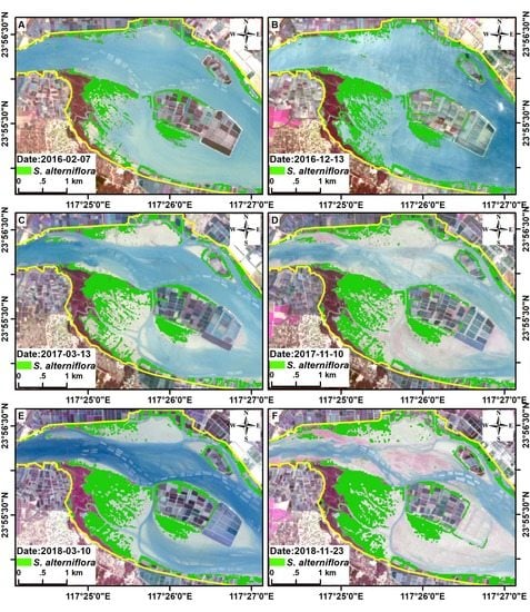
3.3. Temporal and Spatial Changes of S. alterniflora

Spatial dynamics of S. alterniflora from February 2016 to November 2018 are shown in Figure 6. Large patches of S. alterniflora were mainly located in front of mangrove forests along the southern coasts of Zhangjiang Estuary, while a number of small patches were located close to aquaculture ponds. During 2016 to 2018, S. alterniflora patches were found to become more and more aggregated. Newly colonized S. alterniflora clumps are observed among mudflats and mangrove forests.
Temporal changes of S. alterniflora are shown in Figure 7. From 2016 to 2018, S. alterniflora increased dramatically, at a rate of 39.5 ha/year (26.1%). Notable invasions of S. alterniflora are observed both in growing seasons and dormant seasons (Table 5). During the growing seasons of 2016, 2017, and 2018, S. alterniflora increased by 23.1 ha (15.2%, from February to December 2016), 34.3 ha (18.1%, from March to November 2017), and 37.0 ha (15.9%, from March to November 2018), respectively. During the dormant seasons of 2016 to 2017 and 2017 to 2018, S. alterniflora increased by 14.7 ha (8.4%, from December 2016 to March 2017) and 9.5 ha (4.2%, from November 2017 to March 2018), respectively.

4. Discussion

4.1. Advantages of the Data and Methods

Since the late 1990s, monitoring S. alterniflora invasion has received extensive attention [2,9,14,16,23,68]. According to literature review, the overall classification accuracies obtained by this study (ranging from 92% to 95%) are much higher than those of previous research (Table 6). There are two advantages of this study.
First, Sentinel-2 MSI, with fine spatial resolution (up to 10 m), multispectral images (13 bands), and high temporal frequency (2–5 day revisit cycle), improved the capability of detecting S. alterniflora [20,69]. Due to the patchy and narrow pattern of S. alterniflora patches, S. alterniflora derived from 10 m spatial resolution imagery must be more accurate than those from 30 m spatial resolution Landsat imagery. Compared to other high-resolution imagery (for example, SPOT 5), Sentinel-2 imagery has many more spectra bands (10 bands) that can be used in vegetation monitoring, with four red edge bands. Several authors highlighted that separability among vegetation categories has been increased with the introduction of red edge bands and narrow NIR [66,70,71,72]. In particular, some researchers have established indices based on the red band, NIR, and SWIR of remote sensing images to distinguish floating vegetation from water background. One such index is the land surface water index (LSWI), which was built based on the reflectance of NIR and SWIR and is widely used for the remote sensing of surface water from space [73]. The floating algae index (FAI) was defined based on the reflectance of a red band, SWIR, and NIR; it is used to characterize the intense blooms of cyanobacteria [46]. However, these indices are not suitable for discriminating submerged vegetation from water, because there are small variations in the reflectance of submerged vegetation which are suppressed by surrounding water. Compared to these indices, the SAI is a more sensitive index for separating submerged S. alterniflora from water, and it can reduce the impact of unexpected noises from a certain band by using three red edge bands and a narrow NIR of a Sentinel-2 image, according to analysis in Section 2.3. Thus, in this study, the SAI established by the red edge bands successfully extracted submerged patches of S. alterniflora that were overlooked in other studies. Furthermore, repetition cycle of Sentinel-2 imagery provides great opportunities in acquiring dense time series images, which are ideal for monitoring seasonal invasions of S. alterniflora.
Second, based on multiscale optimal segmentation model, we obtained better boundary consistencies between the segmented image objects and real land cover types. Previously, most studies used single-scale optimal segmentation model to identify the spatiotemporal distribution of coastal ecosystems [22]. However, the spatial pattern of land cover in Zhangjiang Estuary is more complex. S. alterniflora patches on the mudflats are patchy and fragmented, while the patches of mangrove forest, water, and aquaculture pond are large and concentrated. Thus, a single segmentation scale is not suitable for land cover delineation. The multiscale optimal segmentation model used in our study gave different optimal segmentation scales for different land covers so that the classification results were more accuarate.

4.2. New Findings of S. alterniflora Invasion Process

For the first time, we found that S. alterniflora invaded significantly during dormant seasons. According to literature, when S. alterniflora entered into a new habitat, in addition to widespread dispersal of seeds, it was able to use the rhizome diffusion to expand the population and enter new pieces of habitat [76]. That means that, although S. alterniflora turns brown during dormant season, it does not stop growing, because the roots are still developing [77]. Our discovery reaffirmed the above knowledge on the S. alterniflora invasion mechanism. To our knowledge, this study is the first attempt to monitor continuous S. alterniflora invasion at multiyear seasonal scales. Most previous studies monitored the extent of S. alterniflora at a chosen day to represent S. alterniflora status for a year. In fact, S. alterniflora follows distinct growth states in different seasons. Thus, our high-temporal-scale spatial dynamics information is of great significance to accurately reflect S. alterniflora invasion process and reveal its potential invasion mechanism.
In addition, by comparing our results with other existing studies of the Zhangjiang Estuary, we concluded that invasion of S. alterniflora has been largely accelerated. According to Liu et al. (2017), the areal extent of S. alterniflora in Zhangjiang Estuary only increased by 3.42 ha from 2003 to 2012, while the invasion accelerated during 2012 to 2015 with an increasing rate of 18.25 ha/year [11]. Results of this study consistently showed that, from 2016 to 2018, the rate of S. alterniflora invasion was 39.5 ha/year. The accelerated invasion has also been found in coastal areas such as Beihai in Guangxi province from 2009 and 2011 and Yueqing in Zhejiang province over the past 21 years [4,36]. Thus, urgent efforts should be taken to manage S. alterniflora invasions.

4.3. Uncertainties

Satellite monitoring has become the major means to map the distribution of S. alterniflora by comparing the spectral discrimination among S. alterniflora and other land cover types [2,4,8,23]. Due to the uncertainties of local instantaneous tidal conditions during predetermined times that satellites pass over, the extent of S. alterniflora may not fully exposed [6]. In this case, the spectral characteristic of the submerged S. alterniflora will be altered and the effectiveness of spectral discrimination for S. alterniflora will be weakened. Thus, high-tide stage can reduce the extent of S. alterniflora mapped because submerged S. alterniflora will be confused with water [38]. In this study, the area of submerged S. alterniflora was determined to be 16.2 ha, meaning that 9.3% of the total area of S. alterniflora is lost due to tidal effects. Therefore, if tidal conditions are not taken into account in the mapping of S. alterniflora, we believe that the monitoring of S. alterniflora will be inaccurate.
In this study, the submerged S. alterniflora was identified by SAI. However, SAI was derived based on the reflectance peak of chlorophyll; as a result, other submerged vegetation and floating vegetation (for example, algae) may be misclassified as S. alterniflora [46,78]. In this case, S. alterniflora may be overestimated. In contrast, it was found that it was difficult to detect typical NIR peaks of vegetation spectra depths of 0.5 m with high turbidity (50 nephelometric turbidity units) and 1 m with low turbidity (0.5 nephelometric turbidity units), [79]. Hence, S. alterniflora submerged by high-turbidity water may be underestimated.
In addition, S. alterniflora shows different spectral characteristics in different seasons, which means that the characteristics of S. alterniflora may be confused with different vegetation in different seasons [75]. For this study, in the dormant seasons, some S. alterniflora were completely withered. Thus, it is difficult to separate S. alterniflora from surrounding mudflats, especially for the small clumps (less than 100 m2) of newly colonized patches. Fortunately, with the production of higher resolution image data, it is possible to solve these problems.

5. Conclusions

In this study, multiyear seasonal Setinel-2 imagery was combined with RF algorithm and OBIA classification method and used to monitor the S. alterniflora invasion process at a continuous seasonal scale during 2016 to 2018. To our knowledge, this is the first study to extract submerged S. alterniflora from the water by developing an SAI derived from reflectance peaks between red edge bands, narrow NIR, and SWIR2 in Sentinel-2 images to remove tide influences. Additionally, a multiscale optimal segmentation was applied to delineate objects during OBIA classification.
Our results showed that: (1) The SAI provided an effective method to extract submerged S. alterniflora from water and increased the overall accuracy of S. alterniflora mapping at high tide to 95%, with a Kappa coefficient of 0.93. (2) Sentinel-2 imagery and multiscale optimal segmentation significantly improved the classification accuracies of S. alterniflora. (3) S. alterniflora dramatically expanded in Zhangjiang Estuary during the period of March 2016 to November 2018, in which the total area increased by 118.6 ha, accounting for 78% of the original areal extent. (4) S. alterniflora spread both in growing seasons and dormant seasons; the average growth rate was 31.5 ha/season during growing seasons and 12.1 ha/season during dormant seasons. In addition, we concluded that the invasion process of S. alterniflora has been largely accelerated by comparing to other existing studies of Zhangjiang Estuary. Methods presented by this study bring great benefits to remote sensing communities of coastal and aquatic vegetation studies. New findings about the S. alterniflora invasion process will contribute to controlling invasion and protecting coastal ecosystems.

Author Contributions

All authors have contributed substantially and uniquely to the work reported. Y.T. and M.J. conceived and designed the research. Y.T. processed the data and wrote the manuscript draft. Z.W., D.M., and C.W. reviewed the manuscript. Y.T. and B.D. took part in the field data collection. All authors have read and agreed to the published version of the manuscript.

Acknowledgments

This study was jointly supported by the National Key Research and Development Program of China (2016YFC0500201); the National Natural Science Foundation of China (41730643); the Youth Innovation Promotion Association of Chinese Academy of Sciences (2017277); the Open Fund of State Laboratory of Information Engineering in Surveying, Mapping and Remote Sensing, Wuhan University (Grant No. 19I02); and the National Earth System Science Data Center (www.geodata.cn).

Conflicts of Interest

The authors declare no conflict of interest.

References

  1. Gao, G.F.; Li, P.F.; Zhong, J.X.; Shen, Z.J.; Chen, J.; Li, Y.T.; Isabwe, A.; Zhu, X.Y.; Ding, Q.S.; Zhang, S.; et al. Spartina alterniflora invasion alters soil bacterial communities and enhances soil N2O emissions by stimulating soil denitrification in mangrove wetland. Sci. Total Environ. 2019, 653, 231–240. [Google Scholar] [CrossRef]
  2. Liu, M.Y.; Mao, D.H.; Wang, Z.M.; Li, L.; Man, W.D.; Jia, M.M.; Ren, C.Y.; Zhang, Y.Z. Rapid Invasion of Spartina alterniflora in the Coastal Zone of Mainland China: New Observations from Landsat OLI Images. Remote Sens. 2018, 10, 1933. [Google Scholar] [CrossRef] [Green Version]
  3. Anttila, C.K.; Daehler, C.C.; Rank, N.E.; Strong, D.R. Greater male fitness of a rare invader (Spartina alterniflora, Poaceae) threatens a common native (Spartina foliosa) with hybridization. Am. J. Bot. 1998, 85, 1597–1601. [Google Scholar] [CrossRef] [PubMed]
  4. Wang, A.Q.; Chen, J.D.; Jing, C.W.; Ye, G.Q.; Wu, J.P.; Huang, Z.X.; Zhou, C.S. Monitoring the Invasion of Spartina alterniflora from 1993 to 2014 with Landsat TM and SPOT 6 Satellite Data in Yueqing Bay, China. PLoS ONE 2015, 10, e0135538. [Google Scholar] [CrossRef] [PubMed] [Green Version]
  5. Li, B.; Liao, C.H.; Zhang, X.D.; Chen, H.L.; Wang, Q.; Chen, Z.Y.; Gan, X.J.; Wu, J.H.; Zhao, B.; Ma, Z.J. Spartina alterniflora invasions in the Yangtze River estuary, China: An overview of current status and ecosystem effects. Ecol. Eng. 2009, 35, 511–520. [Google Scholar] [CrossRef]
  6. Zhu, X.D.; Meng, L.X.; Zhang, Y.H.; Weng, Q.H.; Morris, J. Tidal and Meteorological Influences on the Growth of Invasive Spartina alterniflora: Evidence from UAV Remote Sensing. Remote Sens. 2019, 11, 1208. [Google Scholar] [CrossRef] [Green Version]
  7. Zuo, P.; Zhao, S.H.; Liu, C.A.; Wang, C.H.; Liang, Y.B. Distribution of Spartina spp. along China’s coast. Ecol. Eng. 2012, 40, 160–166. [Google Scholar] [CrossRef]
  8. Lu, J.B.; Zhang, Y. Spatial distribution of an invasive plant Spartina alterniflora and its potential as biofuels in China. Ecol. Eng. 2013, 52, 175–181. [Google Scholar] [CrossRef]
  9. O’Donnell, J.; Schalles, J. Examination of Abiotic Drivers and Their Influence on Spartina alterniflora Biomass over a Twenty-Eight Year Period Using Landsat 5 TM Satellite Imagery of the Central Georgia Coast. Remote Sens. 2016, 8, 477. [Google Scholar] [CrossRef] [Green Version]
  10. Ai, J.Q.; Gao, W.; Gao, Z.Q.; Shi, R.H.; Zhang, C. Phenology-based Spartina alterniflora mapping in coastal wetland of the Yangtze Estuary using time series of GaoFen satellite no. 1 wide field of view imagery. J. Appl. Remote Sens. 2017, 11, 026020. [Google Scholar] [CrossRef]
  11. Liu, M.Y.; Li, H.Y.; Li, L.; Man, W.D.; Jia, M.M.; Wang, Z.M.; Lu, C.Y. Monitoring the Invasion of Spartina alterniflora Using Multi-source High-resolution Imagery in the Zhangjiang Estuary, China. Remote Sens. 2017, 9, 539. [Google Scholar] [CrossRef] [Green Version]
  12. Aguilar, M.A.; Saldaña, M.M.; Aguilar, F.J. Assessing geometric accuracy of the orthorectification process from GeoEye-1 and WorldView-2 panchromatic images. Int. J. Appl. Earth Obs. Geoinf. 2013, 21, 427–435. [Google Scholar] [CrossRef]
  13. Fu, B.L.; Wang, Y.Q.; Campbell, A.; Li, Y.; Zhang, B.; Yin, S.B.; Xing, Z.F.; Jin, X.M. Comparison of object-based and pixel-based Random Forest algorithm for wetland vegetation mapping using high spatial resolution GF-1 and SAR data. Ecol. Indic. 2017, 73, 105–117. [Google Scholar] [CrossRef]
  14. Castillo, J.A.A.; Apan, A.A.; Maraseni, T.N.; Salmo, S.G. Estimation and mapping of above-ground biomass of mangrove forests and their replacement land uses in the Philippines using Sentinel imagery. ISPRS J. Photogramm. Remote Sens. 2017, 134, 70–85. [Google Scholar] [CrossRef]
  15. Verrelst, J.; Muñoz, J.; Alonso, L.; Delegido, J.; Rivera, J.P.; Camps-Valls, G.; Moreno, J. Machine learning regression algorithms for biophysical parameter retrieval: Opportunities for Sentinel-2 and-3. Remote Sens. Environ. 2012, 118, 127–139. [Google Scholar] [CrossRef]
  16. Drusch, M.; Del Bello, U.; Carlier, S.; Colin, O.; Fernandez, V.; Gascon, F.; Hoersch, B.; Isola, C.; Laberinti, P.; Martimort, P. Sentinel-2: ESA’s optical high-resolution mission for GMES operational services. Remote Sens. Environ. 2012, 120, 25–36. [Google Scholar] [CrossRef]
  17. Persson, M.; Lindberg, E.; Reese, H. Tree Species Classification with Multi-Temporal Sentinel-2 Data. Remote Sens. 2018, 10, 1794. [Google Scholar] [CrossRef] [Green Version]
  18. Grabska, E.; Hostert, P.; Pflugmacher, D.; Ostapowicz, K. Forest Stand Species Mapping Using the Sentinel-2 Time Series. Remote Sens. 2019, 11, 1197. [Google Scholar] [CrossRef] [Green Version]
  19. Roy, D.P.; Li, Z.B.; Zhang, H.K.K. Adjustment of Sentinel-2 Multi-Spectral Instrument (MSI) Red-Edge Band Reflectance to Nadir BRDF Adjusted Reflectance (NBAR) and Quantification of Red-Edge Band BRDF Effects. Remote Sens. 2017, 9, 1325. [Google Scholar] [CrossRef] [Green Version]
  20. Jia, M.M.; Wang, Z.M.; Wang, C.; Mao, D.H.; Zhang, Y.Z. A New Vegetation Index to Detect Periodically Submerged Mangrove Forest Using Single-Tide Sentinel-2 Imagery. Remote Sens. 2019, 11, 2043. [Google Scholar] [CrossRef] [Green Version]
  21. Wang, D.Z.; Wan, B.; Qiu, P.H.; Su, Y.J.; Guo, Q.H.; Wang, R.; Sun, F.; Wu, X.C. Evaluating the Performance of Sentinel-2, Landsat 8 and Pléiades-1 in Mapping Mangrove Extent and Species. Remote Sens. 2018, 10, 1468. [Google Scholar] [CrossRef] [Green Version]
  22. Lu, C.Y.; Liu, J.F.; Jia, M.M.; Liu, M.Y.; Man, W.D.; Fu, W.W.; Zhong, L.X.; Lin, X.Q.; Su, Y.; Gao, Y.B. Dynamic Analysis of Mangrove Forests Based on an Optimal Segmentation Scale Model and Multi-Seasonal Images in Quanzhou Bay, China. Remote Sens. 2018, 10, 2020. [Google Scholar] [CrossRef] [Green Version]
  23. Mao, D.H.; Liu, M.Y.; Wang, Z.M.; Li, L.; Man, W.D.; Jia, M.M.; Zhang, Y.Z. Rapid Invasion of Spartina Alterniflora in the Coastal Zone of Mainland China: Spatiotemporal Patterns and Human Prevention. Sensors 2019, 19, 2308. [Google Scholar] [CrossRef] [PubMed] [Green Version]
  24. Proença, B.; Frappart, F.; Lubac, B.; Marieu, V.; Ygorra, B.; Bombrun, L.; Michalet, R.; Sottolichio, A. Potential of High-Resolution Pléiades Imagery to Monitor Salt Marsh Evolution After Spartina Invasion. Remote Sens. 2019, 11, 968. [Google Scholar] [CrossRef] [Green Version]
  25. Belgiu, M.; Drăguţ, L. Random forest in remote sensing: A review of applications and future directions. ISPRS J. Photogramm. Remote Sens. 2016, 114, 24–31. [Google Scholar] [CrossRef]
  26. Du, P.J.; Samat, A.; Waske, B.; Liu, S.C.; Li, Z.H. Random Forest and Rotation Forest for fully polarized SAR image classification using polarimetric and spatial features. ISPRS J. Photogramm. Remote Sens. 2015, 105, 38–53. [Google Scholar] [CrossRef]
  27. Rodriguez-Galiano, V.F.; Ghimire, B.; Rogan, J.; Chica-Olmo, M.; Rigol-Sanchez, J.P. An assessment of the effectiveness of a random forest classifier for land-cover classification. ISPRS J. Photogramm. Remote Sens. 2012, 67, 93–104. [Google Scholar] [CrossRef]
  28. Bassa, Z.; Bob, U.; Szantoi, Z.; Ismail, R. Land cover and land use mapping of the iSimangaliso Wetland Park, South Africa: Comparison of oblique and orthogonal random forest algorithms. J. Appl. Remote Sens. 2016, 10, 015017. [Google Scholar] [CrossRef]
  29. Drǎguţ, L.; Tiede, D.; Levick, S.R. ESP: A tool to estimate scale parameter for multiresolution image segmentation of remotely sensed data. Int. J. Geogr. Inf. Sci. 2010, 24, 859–871. [Google Scholar] [CrossRef]
  30. van Niekerk, A. A comparison of land unit delineation techniques for land evaluation in the Western Cape, South Africa. Land Use Policy 2010, 27, 937–945. [Google Scholar] [CrossRef] [Green Version]
  31. Woodcock, C.E.; Strahler, A.H. The factor of scale in remote sensing. Remote Sens. Environ. 1987, 21, 311–332. [Google Scholar] [CrossRef]
  32. Maghsoudi, Y.; Collins, M.J.; Leckie, D.G. Radarsat-2 Polarimetric SAR Data for Boreal Forest Classification Using SVM and a Wrapper Feature Selector. IEEE J. Sel. Top. Appl. Earth Obs. Remote Sens. 2013, 6, 1531–1538. [Google Scholar] [CrossRef]
  33. Akar, Ö.; Güngör, O. Classification of multispectral images using Random Forest algorithm. J. Geod. Geoinf. 2012, 1, 105–112. [Google Scholar] [CrossRef] [Green Version]
  34. Breiman, L. Random forests. Mach. Learn. 2001, 45, 5–32. [Google Scholar] [CrossRef] [Green Version]
  35. Michez, A.; Piégay, H.; Jonathan, L.; Claessens, H.; Lejeune, P. Mapping of riparian invasive species with supervised classification of Unmanned Aerial System (UAS) imagery. Int. J. Appl. Earth Obs. Geoinf. 2016, 44, 88–94. [Google Scholar] [CrossRef]
  36. Wan, H.W.; Wang, Q.; Jiang, D.; Fu, J.Y.; Yang, Y.P.; Liu, X.M. Monitoring the invasion of Spartina alterniflora using very high resolution unmanned aerial vehicle imagery in Beihai, Guangxi (China). Sci. World J. 2014, 638296. [Google Scholar] [CrossRef] [Green Version]
  37. Campbell, A.; Wang, Y.Q. Examining the Influence of Tidal Stage on Salt Marsh Mapping Using High-Spatial-Resolution Satellite Remote Sensing and Topobathymetric LiDAR. IEEE Trans. Geosci. Electron. 2018, 56, 5169–5176. [Google Scholar] [CrossRef]
  38. Mckee, K.L.; Patrick, W. The relationship of smooth cordgrass (Spartina alterniflora) to tidal datums: A review. Estuaries 1988, 11, 143–151. [Google Scholar] [CrossRef]
  39. Rogers, K.; Lymburner, L.; Salum, R.; Brooke, B.P.; Woodroffe, C.D. Mapping of mangrove extent and zonation using high and low tide composites of Landsat data. Hydrobiologia 2017, 803, 49–68. [Google Scholar] [CrossRef]
  40. Younes Cárdenas, N.; Joyce, K.E.; Maier, S.W. Monitoring mangrove forests: Are we taking full advantage of technology? Int. J. Appl. Earth Obs. Geoinf. 2017, 63, 1–14. [Google Scholar] [CrossRef] [Green Version]
  41. Feng, J.X.; Zhou, J.; Wang, L.M.; Cui, X.W.; Ning, C.X.; Wu, H.; Zhu, X.S.; Lin, G.H. Effects of short-term invasion of Spartina alterniflora and the subsequent restoration of native mangroves on the soil organic carbon, nitrogen and phosphorus stock. Chemosphere 2017, 184, 774–783. [Google Scholar] [CrossRef] [PubMed]
  42. Li, H.Y.; Jia, M.M.; Zhang, R.; Ren, Y.X.; Wen, X. Incorporating the Plant Phenological Trajectory into Mangrove Species Mapping with Dense Time Series Sentinel-2 Imagery and the Google Earth Engine Platform. Remote Sens. 2019, 11, 2479. [Google Scholar] [CrossRef] [Green Version]
  43. Ge, Z.M.; Zhang, L.Q.; Yuan, L. Spatiotemporal Dynamics of Salt Marsh Vegetation regulated by Plant Invasion and Abiotic Processes in the Yangtze Estuary: Observations with a Modeling Approach. Estuaries Coasts 2014, 38, 310–324. [Google Scholar] [CrossRef]
  44. Wang, Q.M.; Blackburn, G.A.; Onojeghuo, A.O.; Dash, J.; Zhou, L.Q.; Zhang, Y.H.; Atkinson, P.M. Fusion of Landsat 8 OLI and Sentinel-2 MSI data. IEEE Trans. Geosci. Remote Sens. 2017, 55, 3885–3899. [Google Scholar] [CrossRef] [Green Version]
  45. Ludwig, C.; Walli, A.; Schleicher, C.; Weichselbaum, J.; Riffler, M. A highly automated algorithm for wetland detection using multi-temporal optical satellite data. Remote Sens. Environ. 2019, 224, 333–351. [Google Scholar] [CrossRef]
  46. Gao, B.C.; Li, R.R. FVI—A Floating Vegetation Index Formed with Three Near-IR Channels in the 1.0–1.24 μm Spectral Range for the Detection of Vegetation Floating over Water Surfaces. Remote Sens. 2018, 10, 1421. [Google Scholar] [CrossRef] [Green Version]
  47. Hossain, M.D.; Chen, D.M. Segmentation for Object-Based Image Analysis (OBIA): A review of algorithms and challenges from remote sensing perspective. ISPRS J. Photogramm. Remote Sens. 2019, 150, 115–134. [Google Scholar] [CrossRef]
  48. Louw, G.; van Niekerk, A. Object-based land surface segmentation scale optimisation: An ill-structured problem. Geomorphology 2019, 327, 377–384. [Google Scholar] [CrossRef]
  49. Rahman, M.R.; Saha, S.K. Multi-resolution segmentation for object-based classification and accuracy assessment of land use/land cover classification using remotely sensed data. J. Indian Soc. Remote Sens. 2009, 36, 189–201. [Google Scholar] [CrossRef]
  50. Chrysafis, I.; Mallinis, G.; Gitas, I.; Tsakiri-Strati, M. Estimating Mediterranean forest parameters using multi seasonal Landsat 8 OLI imagery and an ensemble learning method. Remote Sens. Environ. 2017, 199, 154–166. [Google Scholar] [CrossRef]
  51. Eisavi, V.; Homayouni, S.; Yazdi, A.M.; Alimohammadi, A. Land cover mapping based on random forest classification of multitemporal spectral and thermal images. Environ. Monit. Assess. 2015, 187, 291. [Google Scholar] [CrossRef] [PubMed]
  52. Olofsson, P.; Foody, G.M.; Herold, M.; Stehman, S.V.; Woodcock, C.E.; Wulder, M.A. Good practices for estimating area and assessing accuracy of land change. Remote Sens. Environ. 2014, 148, 42–57. [Google Scholar] [CrossRef]
  53. Mao, D.H.; Wang, Z.M.; Du, B.J.; Li, L.; Tian, Y.L.; Jia, M.M.; Zeng, Y.; Song, K.S.; Jiang, M.; Wang, Y.Q. National wetland mapping in China: A new product resulting from object based and hierarchical classification of Landsat 8 OLI images. ISPRS J. Photogramm. Remote Sens. 2020, 164, 11–25. [Google Scholar] [CrossRef]
  54. Myneni, R.B.; Keeling, C.D.; Tucker, C.J.; Asrar, G.; Nemani, R.R. Increased plant growth in the northern high latitudes from 1981 to 1991. Nature 1997, 386, 698–702. [Google Scholar] [CrossRef]
  55. Mao, D.H.; Wang, Z.M.; Wu, J.G.; Wu, B.F.; Zeng, Y.; Song, K.S.; Yi, K.P.; Luo, L. China’s wetlands loss to urban expansion. Land Degrad. Dev. 2018, 29, 2644–2657. [Google Scholar] [CrossRef]
  56. Zhu, Y.H.; Liu, K.; Liu, L.; Myint, S.W.; Wang, S.G.; Liu, H.X.; He, Z. Exploring the potential of worldview-2 red-edge band-based vegetation indices for estimation of mangrove leaf area index with machine learning algorithms. Remote Sens. 2017, 9, 1060. [Google Scholar] [CrossRef] [Green Version]
  57. He, C.; Li, S.; Liao, Z.X.; Liao, M.S. Texture classification of PolSAR data based on sparse coding of wavelet polarization textons. IEEE Trans. Geosci. Remote Sens. 2013, 51, 4576–4590. [Google Scholar] [CrossRef]
  58. Dell’Acqua, F.; Gamba, P. Texture-based characterization of urban environments on satellite SAR images. IEEE Trans. Geosci. Remote Sens. 2003, 41, 153–159. [Google Scholar] [CrossRef]
  59. Clausi, D.A.; Yue, B. Comparing cooccurrence probabilities and Markov random fields for texture analysis of SAR sea ice imagery. IEEE Trans. Geosci. Remote Sens. 2004, 42, 215–228. [Google Scholar] [CrossRef]
  60. Foody, G.M. Status of land cover classification accuracy assessment. Remote Sens. Environ. 2002, 80, 185–201. [Google Scholar] [CrossRef]
  61. Zhu, Y.H.; Liu, K.; Liu, L.; Wang, S.G.; Liu, H.X. Retrieval of mangrove aboveground biomass at the individual species level with worldview-2 images. Remote Sens. 2015, 7, 12192–12214. [Google Scholar] [CrossRef] [Green Version]
  62. Gitelson, A.A.; Gritz, Y.; Merzlyak, M.N. Relationships between leaf chlorophyll content and spectral reflectance and algorithms for non-destructive chlorophyll assessment in higher plant leaves. J. Plant Physiol. 2003, 160, 271–282. [Google Scholar] [CrossRef]
  63. Wicaksono, P.; Danoedoro, P.; Hartono; Nehren, U. Mangrove biomass carbon stock mapping of the Karimunjawa Islands using multispectral remote sensing. Int. J. Remote Sens. 2016, 37, 26–52. [Google Scholar] [CrossRef]
  64. Korhonen, L.; Packalen, P.; Rautiainen, M. Comparison of Sentinel-2 and Landsat 8 in the estimation of boreal forest canopy cover and leaf area index. Remote Sens. Environ. 2017, 195, 259–274. [Google Scholar] [CrossRef]
  65. Fernández-Manso, A.; Fernández-Manso, O.; Quintano, C. SENTINEL-2A red-edge spectral indices suitability for discriminating burn severity. Int. J. Appl. Earth Obs. Geoinf. 2016, 50, 170–175. [Google Scholar] [CrossRef]
  66. Shoko, C.; Mutanga, O. Examining the strength of the newly-launched Sentinel 2 MSI sensor in detecting and discriminating subtle differences between C3 and C4 grass species. ISPRS J. Photogramm. Remote Sens. 2017, 129, 32–40. [Google Scholar] [CrossRef]
  67. Wang, T.; Zhang, H.S.; Lin, H.; Fang, C.Y. Textural–spectral feature-based species classification of mangroves in Mai Po Nature Reserve from Worldview-3 imagery. Remote Sens. 2016, 8, 24. [Google Scholar] [CrossRef] [Green Version]
  68. Zhang, Y.H.; Huang, G.M.; Wang, W.Q.; Chen, L.Z.; Lin, G.H. Interactions between mangroves and exotic Spartina in an anthropogenically disturbed estuary in southern China. Ecology 2012, 93, 588–597. [Google Scholar] [CrossRef] [Green Version]
  69. Jia, M.M.; Liu, M.Y.; Wang, Z.M.; Mao, D.H.; Ren, C.Y.; Cui, H.S. Evaluating the Effectiveness of Conservation on Mangroves: A Remote Sensing-Based Comparison for Two Adjacent Protected Areas in Shenzhen and Hong Kong, China. Remote Sens. 2016, 8, 627. [Google Scholar] [CrossRef] [Green Version]
  70. Immitzer, M.; Vuolo, F.; Atzberger, C. First Experience with Sentinel-2 Data for Crop and Tree Species Classifications in Central Europe. Remote Sens. 2016, 8, 166. [Google Scholar] [CrossRef]
  71. Schultz, B.; Immitzer, M.; Formaggio, A.; Sanches, I.; Luiz, A.; Atzberger, C. Self-Guided Segmentation and Classification of Multi-Temporal Landsat 8 Images for Crop Type Mapping in Southeastern Brazil. Remote Sens. 2015, 7, 14482–14508. [Google Scholar] [CrossRef] [Green Version]
  72. Sothe, C.; Almeida, C.; Liesenberg, V.; Schimalski, M. Evaluating Sentinel-2 and Landsat-8 Data to Map Sucessional Forest Stages in a Subtropical Forest in Southern Brazil. Remote Sens. 2017, 9, 838. [Google Scholar] [CrossRef] [Green Version]
  73. Chandrasekar, K.; Sesha Sai, M.V.R.S.; Roy, P.S.; Dwevedi, R.S. Land Surface Water Index (LSWI) response to rainfall and NDVI using the MODIS Vegetation Index product. Int. J. Remote Sens. 2010, 31, 3987–4005. [Google Scholar] [CrossRef]
  74. Ai, J.Q.; Gao, W.; Gao, Z.Q.; Shi, R.H.; Zhang, C.; Liu, C.S. Integrating pan-sharpening and classifier ensemble techniques to map an invasive plant (Spartina alterniflora) in an estuarine wetland using Landsat 8 imagery. J. Appl. Remote Sens. 2016, 10, 026001. [Google Scholar] [CrossRef]
  75. Lin, W.P.; Chen, G.S.; Guo, P.P.; Zhu, W.Q.; Zhang, D.H. Remote-Sensed Monitoring of Dominant Plant Species Distribution and Dynamics at Jiuduansha Wetland in Shanghai, China. Remote Sens. 2015, 7, 10227–10241. [Google Scholar] [CrossRef] [Green Version]
  76. Blum, L.K. Spartina alterniflora root dynamics in a Virginia marsh. Mar. Ecol. Prog. Ser. 1993, 102, 169–178. [Google Scholar] [CrossRef]
  77. Gaynor, M.L.; Walters, L.J.; Hoffman, E.A. Ensuring effective restoration efforts with salt marsh grass populations by assessing genetic diversity. Restor. Ecol. 2019, 27, 1452–1462. [Google Scholar] [CrossRef]
  78. Cho, H.J.; Lu, D. A water-depth correction algorithm for submerged vegetation spectra. Remote Sens. Lett. 2010, 1, 29–35. [Google Scholar] [CrossRef]
  79. Liew, S.C.; Chang, C.W. Detecting submerged aquatic vegetation with 8-band WorldView-2 satellite images. In Proceedings of the 2012 IEEE International Geoscience and Remote Sensing Symposium IGARSS, Munich, Germany, 22–27 July 2012; pp. 2560–2562. [Google Scholar] [CrossRef]
Figure 1. Location of study area and spatial distributions of ground survey points.
Remotesensing 12 01383 g001
Figure 2. The submerged S. alterniflora index (SAI) and submerged S. alterniflora pixels. (A) Spectral reflectance curves of mangrove forest, exposed S. alterniflora (E S. alterniflora), submerged S. alterniflora (S. alterniflora), and water in Sentinel-2 image, and baseline of establishing SAI. (B) SAI of the high-tidal Sentinel-2 image. (C) A field photo of S. alterniflora.
Remotesensing 12 01383 g002
Figure 3. The optimal segmentation scales for different objects. (A) Changes in local variance (LV) and rate of change (ROC) with increasing segmentation scale. (B) Segmentation effects with scale parameter of 81. (C) Segmentation effects with scale parameter of 12.
Remotesensing 12 01383 g003
Figure 4. The optimal number and important features. (A) The out-of-bag (OOB) errors and (B) feature importance of the top 13 features.
Remotesensing 12 01383 g004
Figure 5. The distribution of S. alterniflora at high tide, including predicted S. alterniflora derived from SAI (S. alterniflora) and the exposed S. alterniflora (E S. alterniflora).
Remotesensing 12 01383 g005
Figure 6. S. alterniflora distribution maps of the Zhangjiang Estuary from February 2016 to November 2018. Band combination: R:G:B = Sentinel-2 Band 5:4:3.
Remotesensing 12 01383 g006
Figure 7. Coverage area of S. alterniflora from the beginning of the growing season in 2016 to the beginning of the dormant season in 2018.
Remotesensing 12 01383 g007
Table 1. General characteristics of Spectral bands for the Sentinel-2 MultiSpectral Instrument (MSI) sensors.
Sentinel-2 MSI BandsCentral Wavelength (nm)Bandwidth (nm)Spatial Resolution (m)
Coastal aerosol (Band 1)4432060
Blue (Band 2)4906510
Green (Band 3)5603510
Red (Band 4)6653010
Vegetation red edge (Band 5)7051520
Vegetation red edge (Band 6)7401520
Vegetation red edge (Band 7)7832020
Near-infrared (Band 8)84211510
Narrow near-infrared (Band 8A)8652020
Water vapor (Band 9)9452060
Cirrus (Band 10)13803060
Short-wave infrared reflectance (SWIR)1 (Band 11)16109020
SWIR2 (Band 12)219018020
Table 2. Descriptions of selected Sentinel-2 images and instantaneous tide levels.
MissionObservation DateTransit TimeTransit Tidal Height/mTidal Level
Sentinel-2A7 February 201610:49:020.22low
Sentinel-2A13 December 201610:46:522.57high
Sentinel-2A13 March 201710:45:41−1.16low
Sentinel-2B10 November 201710:47:39−1.45low
Sentinel-2B10 March 201810:35:390.06low
Sentinel-2A23 November 201810:48:19−1.67low
Table 3. A list of features for S. alterniflora classification.
Object Features Formula for Sentinel-2
Spectral bandsIndividual BandsB2, B3, B4, B5, B6, B7, B8, B8a, B11, B12
Conventional NIR indicesDVI [61] B 8 B 4
CIg [62] B 8 / B 3 1
SR [61] B 8 / B 4
NDVI [63] B 8 B 4 / B 8 + B 4
EVI [64] 2.5 × B 8 B 4 / B 8 + 6 × B 4 7.5 × B 2 + 1
Red edge indicesCIre1 [65] B 5 / B 3 1
CIre2 [65] B 6 / B 3 1
CIre3 [65] B 7 / B 3 1
NDVIre1 [66] B 8 B 5 / B 8 + B 5
NDVIre2 [66] B 8 B 6 / B 8 + B 6
NDVIre3 [66] B 8 B 7 / B 8 + B 7
MSRren [65] B 8 a / B 5 1 ( B 8 a / B 5 ) + 1
SWIR indicesMDI1 [21] B 8 B 11 / B 111
MDI2 [21] B 8 B 12 / B 12
Geometry featuresDensity D = n 1 + V a r X + V a r Y
Shape index SI = P 4 × A
Area--
Border length--
Length--
Length/width--
Width--
Texture informationHomogeneity [67] i , j = 1 N g G L C M i , j 1 + i j
Contrast [67] i , j = 1 N g i j 2 G L C M i , j
Entropy [67] i , j = 1 N g G L C M i , j 2
Correlation [67] i , j = 1 N g i × j × G L C M i , j μ x μ y σ x × σ y
Table 4. Producer’s and user’s accuracies of S. alterniflora, and overall accuracies and Kappa coefficients of classification results.
AccuracyProducerUserOverallKappa
Time
7 February 20160.940.910.940.92
13 December 20160.930.950.950.93
13 March 20170.940.920.930.91
10 November 20170.940.910.930.92
10 March 20180.930.910.920.89
23 November 20180.920.940.940.91
Table 5. S. alterniflora change during growing season and dormant season from 2016–2018.
StageChange of Area (ha)Change Rate (%)
Growing seasons2016/02/07-2016/12/1323.115.2
2017/03/13-2017/11/1034.318.1
2018/03/10-2018/11/233715.9
Dormant seasons2016/12/13-2017/03/1314.78.4
2017/11/10-2018/03/109.54.2
Table 6. Overall accuracy of S. alterniflora obtained from different sensors and classification methods.
ResearchOverall AccuracyStudy AreaData SourceClassification Method
This study92%–95%Zhangjiang EstuarySentinel-2Multiscale Optimal Segmentation and Random Forest (RF)
Wang et al., 2015 [4]87.4%Yueqing Bay, ChinaSPOT 6Object-Based Image Analysis (OBIA)
Wang et al., 2015 [4]80%–90%Yueqing Bay, ChinaLandsat TMSupport Vector Machine (SVM)
Liu et al., 2017 [11]87%Zhangjiang EstuarySPOT 5OBIA and Visual Interpretation
Liu et al., 2017 [11]86%–90%Zhangjiang EstuaryGoogle EarthOBIA and Visual Interpretation
Liu et al., 2017 [11]87%Zhangjiang EstuaryGoogle Earth and Gaofen-1OBIA and Visual Interpretation
Ai et al., 2016 [74]84.42%Chongming islandLandsat 8 OLIPan-sharpening and Classifier Ensemble Techniques
Lin et al., 2015 [75]87.71%Jiuduansha WetlandZiYuan1 and ZiYuan3Decision Tree Classification

