Article

Impact of Calibrating Filtering Algorithms on the Quality of LiDAR-Derived DTM and on Forest Attribute Estimation through Area-Based Approach

by
Diogo N. Cosenza
1,*,
Luísa Gomes Pereira
2,3,
Juan Guerra-Hernández
1,4,
Adrián Pascual
1,
Paula Soares
1 and
Margarida Tomé
1
1
Forest Research Centre, School of Agriculture, University of Lisbon, Tapada da Ajuda, 1349-017 Lisboa, Portugal
2
Águeda School of Technology and Management (ESTGA), Aveiro University, Apartado 473, 3754-909 Águeda, Portugal
3
Centre for Research in Geospatial Science (CICGE), Porto University, 4099-002 Porto, Portugal
4
3edata, Centro de Iniciativas Empresariais, Fundación CEL, 27004 Lugo, Spain
*
Author to whom correspondence should be addressed.
Remote Sens. 2020, 12(6), 918; https://doi.org/10.3390/rs12060918
Submission received: 29 January 2020 / Revised: 4 March 2020 / Accepted: 10 March 2020 / Published: 12 March 2020
(This article belongs to the Special Issue LiDAR Remote Sensing of Forest Resources and Wildland Fires)

Abstract

:
Ground point filtering of the airborne laser scanning (ALS) returns is crucial to derive digital terrain models (DTMs) and to perform ALS-based forest inventories. However, the filtering calibration requires considerable knowledge from users, who normally perform it by trial and error without knowing the impacts of the calibration on the produced DTM and the forest attribute estimation. Therefore, this work aims at calibrating four popular filtering algorithms and assessing their impact on the quality of the DTM and the estimation of forest attributes through the area-based approach. The analyzed filters were the progressive triangulated irregular network (PTIN), weighted linear least-squares interpolation (WLS) multiscale curvature classification (MCC), and the progressive morphological filter (PMF). The calibration was established by the vertical DTM accuracy, the root mean squared error (RMSE) using 3240 high-accuracy ground control points. The calibrated parameter sets were compared to the default ones regarding the quality of the estimation of the plot growing stock volume and the dominant height through multiple linear regression. The calibrated parameters allowed for producing DTM with RMSE varying from 0.25 to 0.26 m, against a variation from 0.26 to 0.30 m for the default parameters. The PTIN was the least affected by the calibration, while the WLS was the most affected. Compared to the default parameter sets, the calibrated sets resulted in dominant height equations with comparable accuracies for the PTIN, while WLS, MCC, and PFM reduced the models’ RMSE by 6.5% to 10.6%. The calibration of PTIN and MCC did not affect the volume estimation accuracy, whereas calibrated WLS and PMF reduced the RMSE by 3.4% to 7.9%. The filter calibration improved the DTM quality for all filters and, excepting PTIN, the filters increased the quality of forest attribute estimation, especially in the case of dominant height.

Graphical Abstract

1. Introduction

The success of airborne laser scanning (ALS) on collecting accurate measurements of forest ecosystems consolidated this technique worldwide as a state-of-the-art approach in forest inventories. The term ALS refers to light detection and ranging system (LiDAR) onboard an aerial platform, aiming to quickly scan large areas to produce detailed three-dimensional point clouds of the surface [1,2]. These characteristics allow the ALS data to be used for many purposes including topographic- and forest-related studies [3,4,5]. Among the forest-oriented applications, the area-based approach (ABA) has been widely applied to estimate forest attributes, where the tree dominant height and growing stock volume are commonly targeted [6,7,8]. However, the interpretation of ALS data requires successive steps to process, filter and re-scale the information. The calibration of the algorithms used on each step during the processes can turn into a prohibitively time-consuming operation for the users. Furthermore, the experience in handling of the ALS data is essential to properly assess the calibration of the algorithms when it comes, for instance, to generate the digital terrain model (DTM).
Despite the many developments related to the ALS data processing, ground point filtering is a critical procedure for deriving DTM [9], and it is necessary to classify raw ALS returns as coming from the ground or non-ground. Once the ground returns are interpolated to build the DTM (see [10]), the point cloud is normalized in a process by which the Z coordinates of all non-ground returns are re-scaled to above-ground elevation. In the case of the ABA, several metrics are extracted from the normalized point cloud and used to estimate the forest attributes (see, for example, [11]). Thus, the DTM has a great influence on the computation of ALS metrics and consequently on the statistical modeling based on ABA, so the filtering process can be regarded as the cornerstone step in the data processing when using ALS in forest inventory.
Great efforts have been made to develop enhanced filtering algorithms [12]. Besides the quality of the filtering, the usability of an algorithm is partially related to its availability on the ALS-oriented processing software. Among the most common filtering algorithms available, good solutions have been reported when using progressive triangulated irregular network (PTIN, [13]), weighted linear least-squares interpolation (WLS, [14]), multiscale curvature classification (MCC, [15]), or the progressive morphological filter (PMF, [16]).
The performance of the above-mentioned methods has been tested in forest areas where the results point to a higher discrepancy among filters as the terrain becomes steep and as the undergrowth increases [17,18,19]. This fact is common in other benchmarks, which shows the higher difference among the filter efficiencies as the terrain complexity increases [20,21,22,23,24,25]. As presented by Montealegre et al. [26], the steeped slopes affect the way the filters recognize the returns belonging to the vegetation from ones coming from the ground, causing excessive removal of returns and reducing the details of the ground surfaces. Another source of errors in the filtering process is caused by the border effect, which is the misclassification of returns on the border of the dataset due to the lack of returns outside the boundary [21]. Consequently, many returns in the border are removed causing an erosion in the DTM, so that it cannot extend above all non-ground returns. In this regard, the interpolation process of ground returns located on the edge of the ALS coverage is challenging and can substantially impact the quality of the ALS-based inventory workflow.
The filter calibration is often required to improve the filtering performance, where trial and error are the most common praxis. Using and calibrating a filtering algorithm can involve several parameters that may require considerable knowledge from forest practitioners along a tedious and time-consuming process. Many benchmark studies applied parameters calibration to compare filters [18,26], but the practical effects of the calibration on the accuracy of the DTM and the forest attribute estimation are still unknown. This understanding would be valuable for ALS users by supporting them during the data processing to produce the DTM, especially when the forest characterization is the goal.
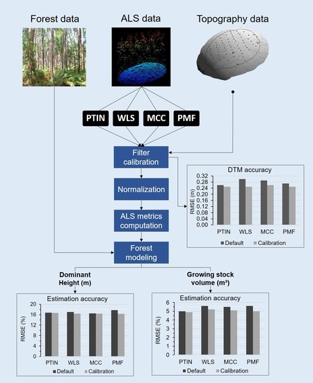
The aims of this study are: i) To assess the calibration of four filtering algorithms (PTIN, WLS, MCC, and PMF) commonly used in ALS-based forest inventory; ii) to evaluate the impact of the calibration on the DTM quality and forest modeling, particularly for plot growing stock volume and dominant height estimation. The analysis was oriented to the forest data users or the ones who need to process ALS data of forested areas. We applied alternative combinations of parameter values for each tested algorithm in the software implementation, and the different parameters were calibrated according to the accuracy of the DTM derived from the filtered ground returns. More than 3000 ground control points were used to assess the quality of the produced DTM. The effect of calibrating the filters was traced from the DTM generation to its impact on the performance of the models, where the multiple linear regression approach and a eucalyptus forest plantation was used as showcase.

2. Material and Methods

2.1. Study Area

The study area is located in Northwest Portugal (40°36′N, 8°25′W), close to the city of Águeda, comprising 9 km2 of forested landscapes. The terrain presents a heterogenic topography, with altitude varying from 70 to 220 m and slopes ranging from 2.5% to 34.2%. At the time of the forest data collection (July 2008), the forest area was mainly covered by pure even-aged Eucalyptus globulus Labill stands, harvested every 10–12 years during three or four rotations, with some stands of Pinus pinaster Aiton. The eucalyptus stands had a mean tree density around 1600 trees per hectare, with regular or irregular spacings, and they were composed by stands from seedling (first rotation) and regenerated by coppice (following rotations) for pulp supplying. Many stands were multi-layered, with E. globulus in the uppermost layer and suppressed trees, shrubby and herbaceous vegetation in the lowermost layer.

2.2. Field Data Collection

The forest and the topographic surveys occurred between 10 June and 3 July 2008 through 41 circular plots with 400 m² of area (11.28 m of radius). The plots were systematically installed over the area (Figure 1a) and covered a large range of terrain slopes (Figure 1b). Within each plot, the diameters at breast height (dbh, at 1.30 m height) were measured from all trees higher than 2 m, together with the height of the dominant and co-dominant trees. For each plot, a concentric subplot of 200 m² (7.98 m of radius) was used to collect the heights of all trees higher than 2 m. The missing tree heights of each plot were estimated using the Prodan’s model [27] fitted with the respective subplot data. The individual tree volumes with bark were estimated using an equation provided by Tomé et al. [28], and the tree volumes were summed to obtain the ground reference volume for each plot (V, m³). The 41 plots were used for the filter calibration assessment, from which 25 plots were selected to evaluate the impact of the calibration on the forest modeling. The selection of the 25 plots was needed to remove plots that were located in the transition boundary between two stands, or crossed by roads, that could bias the forest modeling (see [29]). The biometrical description of the forest content within plots is presented in Table 1.
The coordinates of each tree within each plot were recorded as well as the coordinates of prominent terrain points, like breaklines or spot heights (Figure 1c), resulting in 3240 ground control points, a mean of 79 points per plot (σ = 24). The accuracy of the coordinates of points using a geodetic Global Navigation Satellite Systems (GNSS) on land covered with dense vegetation is not reliable; therefore, the devised strategy for measuring the coordinates of ground control points was not straightforward. Firstly, those coordinates were measured in each plot by means of a topographic survey using the radial method [30]. As these coordinates are in a local system, they were converted to that of the LiDAR data by using GNSS receivers. To this end, it was decided to attach to each plot two GNSS-derived points, named GNSS base, whose coordinates were measured with two GNSS receivers. They allow for coordinating the surveyed points directly in the referred coordinate system. Two points are needed to orient the total station. These two points were placed as close as possible to the plot and as much as possible in an open space. The method used to measure the coordinates of the two GNSS-derived points was the relative positioning by using a fixed receiver on a geodetic pillar with known coordinates on the same system as the LiDAR data. This method, in post-processing, is the most precise and may reach levels of precision in the order of centimeters [31].

2.3. ALS Data Collection and Pre-Processing

The ALS survey was carried out in July 2008, a few days after the forest inventory, using a LiteMapper-5600 laser system from RIEGL (www.riegl.com), which has as main components the high-resolution laser scanner LMS-Q560, the positioning system AEROcontrol, and the digital camera DigiCAM (see [32] for more technical details on the system). The airplane flew 600 m above ground with a mean speed of 46.26 m s−1. The parameters of the laser system were: 0.5 mrad of beam divergence, ±45º of scan angle and pulse rate of 150 kHz. The resulted swath was 497 m (60% of overlap) and the returns density was 9.5 returns m−2. More details about the ALS survey is described in [31,33]. The ALS point clouds were inspected for outliers and further clipped using the plot center coordinates with a 15-m radius buffer (706.85 m²) for each plot. The clipping process was carried out to avoid edge-effect over the ground returns during the filtering process. The FUSION software V3.60 [34] was used for this pre-processing.

2.4. Filtering Calibration

The used filters were chosen based on their recurrent utilization on the related literature [20,26]. We gave preference to those filters implemented into line-code-based software that allows being incorporated into programming routines; in our case the R environment [35] was used. Each filter was applied to the last returns of the point clouds of the 41 plots using different parameter sets. The choice of which parameters to be calibrated was done for each filter since they follow different principles described in the following sections. This work is focused on the filtering process for forest applications, so settings regarding urban terrain or smoothing filters were not considered. The values tested in the calibration were defined considering the ones close to the software defaults and recommendations (Table 2).

2.4.1. Progressive Triangulated Irregular Network (PTIN)

The PTIN is frequently applied in forest studies [36,37,38]. The algorithm starts with a sparse triangulated irregular network (TIN) created from seed points and then performs the densification of the TIN iteratively. In this process, the densification occurs by including the returns according to their distance to the TIN facets and their angles to the nodes. We used the adaptation of PTIN of the LASground software (rapidlasso.com), which comprises the following three assessed parameters: Spike, which is the threshold at which spikes get removed; step size, defines the size of the initial search window and it is dependent on the terrain roughness, where values around 5 are suggested for forest or mountain areas; and granularity, related to the computational effort invested into finding the initial ground estimate.

2.4.2. Weighted Linear Least-Squares Interpolation (WLS)

The applied WLS filter was the adaptation of the Kraus and Pfeifer’s algorithm [14] into the FUSION software [34], which was used in many works [39,40,41]. This filter averages reiteratively the return heights inside a defined search window, assigning the weights according to their residuals in relation to the mean height. In this case, the weights are recalculated in each iteration according to the weighting function (Equation (1)), so that height values associated with lower residuals receive higher weights, whereas those with higher residuals receive lower weights. The parameter values a = 1 and b = 4 are commonly used and are recommended by the software developers for most applications so they were kept in the analysis [14,26]. The parameters g, w, window size and the number of iterations (iteration) are supposed to be defined by the user according to the data, thus they were chosen to be calibrated (Table 2). Among these parameters, the window size is the only one without a specified default value, although the software’s manual points to 5 m². In this case, a window size equal to 5 m² was considered as a default value.
p i = { 1 v i g 1 1 + a ( v i g ) b g < v i g + w   , 0 v i > g + w
where pi is the weight for the return i = 1, …, n; vi is the residual point height value from the average height, being i = 1, …, n; the parameters a and b determine the steepness of the weight function; g is negative and represents a threshold value after which the weights are set to 1 if vi ≤ g and to 0 if vi > g + w. Note that w ≤ |g| for all w values.

2.4.3. Multiscale Curvature Classification (MCC)

The MCC is a filter developed by Evans and Hudak [15] and implemented in MCC-LIDAR software (sourceforge.net/projects/mcclidar). It uses the thin-plate spline interpolation to produce surfaces in different resolutions and uses progressive curvature tolerances to eliminate non-ground returns. The software uses only two parameters that should be set by the user: the initial scale (λ), related to the search window size that is used to interpolate the points; and the initial curvature tolerance (t), which accounts for slope interaction between the interpolated surface and the returns. During the processing, both parameters are changed through three domains to address variable canopy configurations and their interaction with the terrain slope: the initial value set to λ is multiplied by 0.5, 1, and 1.5, while 0.1 is added to the initial t in each domain. Values for λ =1.5 and t = 0.3 are claimed by the developers as efficient to filter non-ground returns, so variations around those values were tested in this work (Table 2). Applications of the MCC in forest studies can be found, for example, in [42,43,44].

2.4.4. The Progressive Morphological Filter (PMF)

The PMF filter was developed by Zhang et al. [16] and uses concepts of object identification in grey-scale images by applying mathematical morphology filters like opening and closing operators. The closing operator removes returns from objects of sizes smaller than the window size, while the opening operator keeps the returns from larger objects. The PMF was applied using the implementation of the lidR package [45], where the filter works at point cloud level without any rasterization process. The PMF has been commonly applied to ALS data [18,26], and the release of the lidR package has also promoted this filter to process photogrammetric point clouds [46]. The package uses two parameters: the sequence of windows size, and the sequence of threshold, which is the height value below which a return is classified as a ground return. In this study, the PMF was applied using not a sequence but a specific value for each parameter to better isolate the effect of each component in the processing of the ALS datasets (Table 2).

2.5. Filtering Accuracy Assessment

For each combination of filter parameters, the classified ground returns within each plot were interpolated into a DTM (1.0 m of cell size) from a TIN surface using the grid_terrain command implemented on the lidR package [45]. The choice of using the TIN interpolation was due to its efficiency and frequent application to generate DTM from ALS data [9,19,47]; thus, eventual errors in the interpolation were not considered in this analysis. Each combination of the filter parameters was assessed using the root mean squared error (RMSE, Equation (2)) computed with the height values interpolated from the derived DTM at the same planimetric positions as the ground control points. Note that the DTM was generated for each plot separately to allow detecting DTM erosion, which was defined here as the non-inclusion of all ground control points within the DTM extension of its respective plot (Figure 1d). The efficiency of a filtering process was then evaluated using the accuracy of the DTM (the lower the RMSE, the better) so as its integrity, where the erosions were not allowed.
RMSE = i = 1 n ( y i y ^ i ) 2 n
where, y i and y ^ i are, respectively, the observed and estimated value for the observation i = 1, …, n.

2.6. Forest Modeling Assessment

The calibrated parameter values for each filter were further benchmarked against the default values by assessing the impact of the corresponding derived DTM on the estimation of forest attributes through ABA. Each of these DTM was used further into the normalization process, which provided the height of points above ground. The growing-stock volume (V, m³) and the dominant height (hd, m) were estimated for each plot using ALS metrics since these attributes are frequently assessed in the ALS applications. The ALS metrics were computed for each plot using its respective normalized point cloud and considering only points higher than 1 m above ground. The normalization and the computation of ALS metrics were performed using the lidR package [45]; the set of metrics (Table 3) were used as candidate predictors in forest modeling.
Although there are several methodologies to perform a forest attribute modeling [48], the multiple linear regression fitted using ordinary least squares was used as a showcase for its simplicity, efficiency and frequent application to ALS data [49,50,51,52]. Thus, the multiple linear model (Equation (3)) was used to estimate each forest attribute (V and hd), where the two metrics were selected through exhaustive search.
Y = β 0 + β 1 x 1 + β 2 x 2 +   ε
where, Y is the response variable; βi is the model parameter i = 0, 1, 2; xi is the predictor i = 1, 2; and ε is the random error.
Despite this analysis focusing on the estimative efficiency of the models (no inference made), the linear regression assumptions were taken into account. The response variable was square rooted to avoid heteroscedasticity, and the residual variance component was added to the back-transformed response variable when an equation was used to estimate a forest attribute: Y ^ = ( Y ^ ) 2 + σ 2 [8,53]. In the exhaustive search, all possible combinations of two candidate metrics were used to fit the models using the above-mentioned dataset with 25 plots. The best model was considered to be the one with the lowest RMSE (Equation (2)), all parameters significantly different from zero (t-test, α = 5%), and with variance inflation factors lower than 10 [54] computed using the car package [55]. The RMSE was chosen for this purpose for is has been proven to be a stable and robust measure to assess model performances [52].
Each model was selected and fitted using the data from the 25 plots referred above. The fitted equation was assessed through 5-fold cross-validation. In the cross-validation the dataset is split into five sets (“folds”) of equal size to start an iterative process. In each iteration one fold is omitted from the model fitting and has their values estimated by the model; the estimated values of all omitted folds at the end of the process are used to compute the final error. The entire cross-validation was repeated 100 times to reduce the randomness involved in this process [56]. Thus, the resultant RMSE values from the calibrated filter were compared to the ones derived from the default values through the Wilcoxon–Mann–Whitney test [57,58], since preliminary analysis demonstrates that the RMSE values were not normally distributed. The accuracy of the models was thus represented by the median of the error values (RMSEmed) as well as its percentage from the observed mean values RMSE%med.

3. Results

3.1. Filtering Parameters Calibration

As a general result, the calibration of the filter parameters allowed to produce more accurate DTMs than those produced using the software defaults, with RMSE from 0.25 to 0.26 m when calibrated, against a variation from 0.26 to 0.30 m with the default (Table 4). The accuracy of the DTMs produced with the calibrated PTIN had the smallest improvement when compared to that obtained by using the default parameters (a reduction of 4% in the RMSE). On the other hand, the accuracy of the DTMs produced with calibrated WLS had the highest improvement on accuracy, decreasing 16% in terms of RMSE. Excepting the PMF, the filters have more than one calibrated parameter set, so the set that has less impact on the computational effort was chosen.
The tested parameters of PTIN resulted in a small variation in the accuracy of DTMs, with RMSE ranging from 0.25 to 0.29 m (Figure 2). The DTM accuracy was less affected by the spike and most influenced by the step size—the RMSE decreased continually as the step size increased. On the other hand, larger values for step size increased the susceptibility of the filter to border effect, producing eroded DTMs. This effect was intensified when the coarse granularity was applied so that smaller values of step size were needed to derive eroded DTMs. Despite the influence of the border effect, the granularity had marginal impact on the accuracy of the DTMs, and the fine and extra fine granularity had comparable results. Therefore, the fine granularity should be preferred since it requires less computational effort during data processing.
The WLS presented high variation in the DTM accuracy among the different parameter settings (RMSE between 0.25 and 0.46 m). It is strongly and similarly affected by the parameters g and w (Figure 3), where the RMSE decreased with their decreasing in value. Additionally, the RMSE decreased as the differences in the absolute values of these parameters decreased, which means that the filter is more accurate as |g| and w values are closer. The tested number of iterations and window cell sizes did not influence the accuracy of the DTMs, but they were important concerning the border effect. Eroded DTMs occurred when |g| = w, except when the cell size was set to 1 m² and using three or five iterations. By setting |g| = w the filter is forced to consider only the lowest residuals to compute the averages, and positive residuals (v) are no longer accepted. Consequently, the WLS becomes less tolerant of variations in the ground surface within the search window so more points are removed if a higher cell size or a higher number of iterations are used. Furthermore, there was no difference in the filtering performance when the number of iterations was set to either three or five, so the lower value (i.e., three) should be preferred to speed up the computational process.
The calibration of the MCC did not produce eroded DTMs, and their accuracy varied between 0.26 and 0.36 m (Figure 4). The tolerance had the greatest impact on the filter’s performance (i.e., the higher its value, the higher the RMSE and thus the smaller the DTM accuracy). On the other hand, the scale appears to have only marginal impact, tending to reduce the RMSE as the values increase. The tested values for scale suggested that its effect on the DTM accuracy also depends on the tolerance; when the tolerance was set to 0.1, the effect of the scale on the accuracy was marginal (RMSE between 0.26 and 0.27 m), while a wider range was observed for intermediary tolerance values (e.g., RMSE between 0.29 and 0.34 m for tolerance value equal to 0.4). Despite the most accurate DTM being produced when setting tolerance to 0.1, many values could be used for the scale (0.1–4.5). This parameter controls the cell resolution of the thin-plate spline interpolation (see Section 2.4.3), so setting larger values increases the number of returns to be interpolated. For this reason, using lower values for the scale (i.e., between 1 to 2) is advisable to reduce the computational effort.
The calibration of the PMF parameters resulted in the widest range of DTM accuracies, with RMSE between 0.25 and 0.56 m (Figure 5). Both tested parameters influenced the filtering efficiency. The RMSE of the DTMs increased with the increasing of the threshold. The changes in the accuracy due to the window size were more highlighted when its values shifted from 1 to 3, but a marginal effect was noted for values higher than three. The eroded DTMs were more frequent as the threshold value was lower and the window size higher. Since the PMF uses a sequence of window size values in the filtering, the use of higher values (i.e., ≥9) showed to be not effective for the filtering efficiency in the studied area.

3.2. Estimation of Forest Attributes

The default and the calibrated parameter values listed in Table 4 were used to estimate the forest attributes through ABA. The parameters with more than one calibrated value were set as follows: Fine granularity for PTIN; g = 0 and w = 0 for WLS; and scale = 1.0 for MCC.
The dominant height equations resulted in good accuracy for all filters, with RMSE%med between 4.9% and 5.2% for the calibrated values, and between 5.0% and 5.6% for the default values (Table 5). The calibrated and the default parameters values originated equations with comparable performances for the PTIN considering a confidence level (α) of 5%. The metrics used by the equations derived from PTIN were also similar; the equation derived from the calibrated parameters used Z65, while the one derived from the default parameters used Z60. The calibration of WLS, MCC and PFM resulted in a significant improvement of the estimated dominant height accuracy when compared to that one derived using the default parameter values. The decrease in the RMSEmed values due to the calibration was 0.08 m points for WLS, 0.06 m for MCC and 0.10 for PMF, which are equivalent to an improvement of 8.5%, 6.5% and 10.6%, respectively. Although their respective equations used the metric Z95, the ones derived for the calibrated values used Z60 instead of C8 in the equations of the default values, which are metrics computed with different principles (see Table 3).
Regarding the volume estimation, the models presented RMSE%med between 16.3% and 16.7% when using the calibrated values and 16.5% and 17.7% when using the default values (Table 6). Although these errors are higher than those encountered in the estimation of the dominant height, they could be considered low in the case of volume modeling when assessed through cross-validation. The estimation efficiency when using the calibrated PTIN and MCC did not differ from those derived with filters using their respective default values. The use of WLS and PMF with calibrated parameters significantly improved the volume estimation when comparing to their respective default values. Despite the related equations used the same metrics, the decrease of the RMSEmed values by using the calibrated parameters were 0.018 m³ for WLS and 0.044 m³ for PMF, which is equivalent to an improvement of 3.4% and 7.9%, respectively.

4. Discussion

This study demonstrated that a DTM derived from ALS is more accurate when the parameters of the filtering process are calibrated. The DTM produced with the WLS was the most affected by the calibration, followed by that of the MCC, PMF and of the PTIN (less affected). This fact influenced the estimation of forest attributes, especially for dominant height. Except for PTIN, the estimation of the dominant height derived by using the calibrated parameter values was significantly more accurate than those that are derived with the default ones. In the case of the volume estimation, the calibration of WLS and PFM derived equations with significantly better accuracies, contrary to the PTIN and MCC filters that performed comparably when using calibrated and default parameter values.
The lower effect of the calibration for PTIN is justified by the similarity between the calibrated and the default parameters values, which differs only by 0.5 in the spike parameter value (see Table 2 and Table 4). The calibrated parameters for the MCC differed the most with respect to the default ones, having a large impact on the dominant height estimation as opposed to the volume estimation. The result shows that a DTM can have different impacts on the modeling of these forest attributes and that the calibration will lead to the best results depending on the filter and on the attribute to be estimated.
Although these two forest attributes are highly correlated, they present different aspects when are estimated through ALS data. Many works have reported good correlations between the tree height attributes with upper-tail percentiles of the height distribution of ALS returns [59,60]. The literature is less consensual for the case of the volume estimation, for which good performances are found based on ALS metrics associated to intermediary percentiles (higher than 50%), density metrics (e.g., C8) and/or height variability measures (e.g., height kurtosis) [6,44,50]. These characteristics were also observed in our work, where the metric Z95 appears in all dominant height equations just as the Zmax and C2 in the volume equations. However, studies focusing on the effect of point density over the metrics demonstrated that those ones related to the tail ends of the return distribution (e.g., C1 and C9, or Zmin and Zmax) are more sensible and, therefore, less stable [61]. Despite the point density remaining constant in our analysis, it is possible that those same metrics are also more sensitive to variations in the normalized point cloud due to errors in the DTM. This fact is important in the case of ordinary least squares regression since the predictors are selected following several rules to match the regression assumptions, so small variations in the metric values have unpredictable effects in the final model.
It should be highlighted that the quality of the estimation of stand attributes is strongly dependent on the applied modeling approach [52]. Nonparametric models, such as k-nearest neighbors or random forest, have the advantage of being distribution-free and are normally used with more predictor variables to improve their accuracy [48,62,63]. In this case, it is reasonable to suspect that using more variables would turn the models less vulnerable against changes in the metrics and, thus, the effect of the filter calibration could be hidden by an improvement in the performance of the models. However, the non-parametric approaches require a higher amount of field data for the modeling, which is not often available (as is the case of this work). Besides, traditional parametric modeling approaches have shown to be less affected by biased normalized point clouds, for instance, due to co-registration errors, so that alternative combinations of ALS metrics models can result in similar estimative efficiency [51]. The co-registration effect could be ignored in this work given the high-accurate plot positioning throughout the data collection; therefore, it corroborates that DTM quality is the major factor affecting the performances of the model in the benchmark.
The researches focused on calibration of the above tested filters are scarce in the literature and the few examples were oriented to digital aerial photogrammetry (DAP, [64,65]). One of them is the study of Graham et al. [66] who analyzed the PTIN, WLS and the simple morphological filter (SMRF, see [67]), which works similarly to the PMF. Their results share some similarities with ours: the PTIN was mostly affected by the step size parameter, while the spike had minor or no effects over the accuracy of the derived DTM; the WLS had the best accuracy with the |g| close to w; and low threshold for the SMRF (analogous in PMF). On the other hand, the parameters related to the size of the search windows of these filters (i.e., window size and step size) were exceptionally higher (≥17 m²). However, we have demonstrated that using larger values for these parameters over ALS point clouds increases the susceptibility of the filters to the border effect, resulting in eroded DTM.
The PTIN was also analyzed by Wallace et al. [68] using DAP-based data, where the calibration was performed for different ecosystems. However, in contrast to the study of Wallace et al. [68], our work did not distinguish the areas regarding the terrain conditions or forest covers due to a lack of data for this discretization, especially in the forest modeling assessment. Instead, the filters were analyzed considering all ALS data available so the results of the calibration can be applied to a wider range of forest conditions. Furthermore, many works have been applied the ABA to mountainous sites with success, demonstrating that the impact of the terrain slope over the forest attribute estimation is not significant as expected [60,69,70], thereby it is unlikely that this effect can also compromise the performances of our forest models.
Most of the ground filtering benchmarks assess the accuracy through visual inspection of the filtered ground returns, which allows accounting for omission and commission errors of the filtering [20,21,26]. Although such analysis produces detailed information about the filtering process, it is highly time-consuming and can be impracticable in terms of the calibration routines like the ones performed in this study. The analysis based on the quality of DTM is thus a good and practical alternative when high-accurate ground control data is available. Additionally, further benchmarks should also account for DTM erosion, since it is prohibitive when the goal is forest modeling.
Although this work did not aim at comparing filters, it should be highlighted that all tested filters had comparable performances after the calibration, considering the accuracy of the derived DTM. This fact suggests that more efforts should be given to calibrate the ground point filters instead of finding a better one. Therefore, the software developers must be encouraged to implement adaptive filters to reduce the number of parameters to be set to process the data (e.g., [24,71,72]).
The improvement in the estimation of dominant height is of great importance for forest management since it ensures a more accurate analysis of forest site productivity [59,73]. Likewise, ALS-based models play a key role in the valuation of growing stock inventory [74,75], so reducing the errors of the estimated attributes by calibrating the filters allows increasing the liability of the assessments. However, ALS-data users must preliminarily consider the potential improvement on the DTM accuracy and forest attribute estimation before deciding to calibrate it instead of using the software’s default.
This work did not consider the impact of the errors originating from different interpolation methods on the accuracy of DTM nor on the forest attribute estimation. Previous studies demonstrated the difference among the efficiency of interpolators while deriving DTM from ALS data [19,47]; despite the TIN approach usually performed the best, Stereńczak et al. [19] showed that the differences among the interpolators were reduced after calibration. Additionally, Graham et al. [76] tested several interpolation methods using DAP-data and showed that they do not have significant differences regarding the accuracy of estimated forest attributes. The same may occur in the case of ALS-data, but proper research is needed to investigate such a hypothesis. Finally, our analysis was based on a massive ground control dataset that was collected using an exhaustive and high-accurate topographic survey, which supports the liability of the DTM accuracy assessment [77]. For this reason, our results can be used as a rule of thumb and the information we provided from the filter calibration can guide the user during the ALS data processing, especially if the estimation of forest attributes is the goal.

5. Conclusions

The calibration of four algorithms to filter ground returns of airborne laser scanning data were assessed, namely, the progressive triangulated irregular network (PTIN), weighted linear least-squares interpolation (WLS), multiscale curvature classification (MCC) and the progressive morphological filter (PMF). The impact of the calibration was assessed on the quality of the digital terrain models (DTM) and on the forest attribute estimation accuracy, where the area-based approach (ABA) was applied. The conclusions of this work are:
-
The calibration of the ground filter parameters improved the quality of the DTM.
-
The calibrated parameter values for WLS, MCC, and PMF allowed deriving more accurate estimated forest attributes than those obtained when filtering using their default counterparts, with a more highlighted impact on the estimation of dominant height than of growing stock.
-
The results derived when using the PTIN filter varied the least with the calibration of the parameters.

Author Contributions

Conceptualization, D.N.C. and L.G.P.; Methodology, D.N.C., L.G.P., J.G.-H. and A.P.; Data Analysis, D.N.C. and J.G.-H.; Data Curation, D.N.C., L.G.P., P.S., and M.T.; Investigation, D.N.C., L.G.P., J.G.-H., A.P., P.S., and M.T.; Resources, L.G.P., P.S., and M.T.; Writing—Original Draft Preparation, D.N.C., L.G.P., J.G.-H. and A.P.; Writing—Review and Editing, D.N.C., L.G.P., J.G.-H., A.P., P.S., and M.T.; Funding Acquisition, M.T., P.S., L.G.P.; and Supervision, P.S. and M.T. All authors have read and agreed to the published version of the manuscript.

Funding

The research activities of Diogo Cosenza was funded by Fundação para a Ciência e a Tecnologia I.P. (FCT), grant number PD/BD/128489/2017. Adrián Pascual (I.P. in the scope of Norma Transitória–DL57/2016/CP5151903067/CT4151900586) was supported by Fundação para a Ciência e a Tecnologia through the MODFIRE project—A multiple criteria approach to integrate wildfire behavior in forest management planning (PCIF/MOS/0217/2017). The ALS and field data used in this work were acquired under the framework of the PTDC/AGR-CFL/72380/2006 project (supported by the FCT under grant PTDC/AGR-CFL/72380/2006, co-financed by the European Fund of Regional Development (FEDER) through COMPETE—Operational Factors of Competitiveness Program, POFC). This research was funded by the Forest Research Centre, a research unit funded by Fundação para a Ciência e a Tecnologia I.P. (FCT), Portugal (UIDB/00239/2020).

Acknowledgments

We thank the Fundação para a Ciência e a Tecnologia I.P. (FCT) for funding the research activities of Diogo Cosenza and Adrián Pascual.

Conflicts of Interest

The authors declare no conflicts of interest.

References

  1. Wehr, A.; Lohr, U. Airborne laser scanning—An introduction and overview. ISPRS J. Photogramm. Remote Sens. 1999, 54, 68–82. [Google Scholar] [CrossRef]
  2. Vauhkonen, J.; Maltamo, M.; Mcroberts, R.E.; Næsset, E. Forestry Applications of Airborne Laser Scanning; Maltamo, M., Næsset, E., Vauhkonen, J., Eds.; Managing Forest Ecosystems; Springer: Dordrecht, The Netherlands, 2014; Volume 27. [Google Scholar]
  3. Eitel, J.U.H.; Höfle, B.; Vierling, L.A.; Abellán, A.; Asner, G.P.; Deems, J.S.; Glennie, C.L.; Joerg, P.C.; LeWinter, A.L.; Magney, T.S.; et al. Beyond 3-D: The new spectrum of lidar applications for earth and ecological sciences. Remote Sens. Environ. 2016, 186, 372–392. [Google Scholar] [CrossRef] [Green Version]
  4. Nelson, R. How did we get here? An early history of forestry lidar. Can. J. Remote Sens. 2013, 39, S6–S17. [Google Scholar] [CrossRef] [Green Version]
  5. Hyyppä, J.; Hyyppä, H.; Leckie, D.; Gougeon, F.; Yu, X.; Maltamo, M. Review of methods of small-footprint airborne laser scanning for extracting forest inventory data in boreal forests. Int. J. Remote Sens. 2008, 29, 1339–1366. [Google Scholar] [CrossRef]
  6. Nilsson, M.; Nordkvist, K.; Jonzén, J.; Lindgren, N.; Axensten, P.; Wallerman, J.; Egberth, M.; Larsson, S.; Nilsson, L.; Eriksson, J.; et al. A nationwide forest attribute map of Sweden predicted using airborne laser scanning data and field data from the National Forest Inventory. Remote Sens. Environ. 2017, 194, 447–454. [Google Scholar] [CrossRef]
  7. Næsset, E. Area-based inventory in Norway—From innovation to an operational reality. In Forestry Applications of Airborne Laser Scanning; Maltamo, M., Næsset, E., Vauhkonen, J., Eds.; Springer: Dordrecht, The Netherlands, 2014; pp. 215–240. [Google Scholar]
  8. Kotivuori, E.; Korhonen, L.; Packalen, P. Nationwide airborne laser scanning based models for volume, biomass and dominant height in Finland. Silva Fenn 2016, 50, 1–28. [Google Scholar] [CrossRef] [Green Version]
  9. Liu, X. Airborne LiDAR for DEM generation: Some critical issues. Prog. Phys. Geogr. Earth Environ. 2008, 32, 31–49. [Google Scholar]
  10. Chen, Z.; Gao, B.; Devereux, B. State-of-the-art: DTM generation using airborne LIDAR data. Sensors 2017, 17, 150. [Google Scholar] [CrossRef] [Green Version]
  11. Næsset, E. Practical large-scale forest stand inventory using a small-footprint airborne scanning laser. Scand. J. For. Res. 2004, 19, 164–179. [Google Scholar] [CrossRef]
  12. Meng, X.; Currit, N.; Zhao, K. Ground filtering algorithms for airborne LiDAR data: A review of critical issues. Remote Sens. 2010, 2, 833–860. [Google Scholar] [CrossRef] [Green Version]
  13. Axelsson, P. DEM generation from laser scanner data using adaptive TIN models. In Proceedings of the International Archives of Photogrammetry and Remote Sensing. XIXth ISPRS Congress, Amsterdam, The Netherlands, 16–23 July 2000; Schenk, T., Vosselman, G., Eds.; International Society for Photogrammetry and Remote Sensing: Amsterdam, The Netherlands, 2000; Volume XXXIII, pp. 110–117. [Google Scholar]
  14. Kraus, K.; Pfeifer, N. Determination of terrain models in wooded areas with airborne laser scanner data. ISPRS J. Photogramm. Remote Sens. 1998, 53, 193–203. [Google Scholar] [CrossRef]
  15. Evans, J.S.; Hudak, A.T. A multiscale curvature algorithm for classifying discrete return LiDAR in forested environments. IEEE Trans. Geosci. Remote Sens. 2007, 45, 1029–1038. [Google Scholar] [CrossRef]
  16. Zhang, K.; Chen, S.C.; Whitman, D.; Shyu, M.L.; Yan, J.; Zhang, C. A progressive morphological filter for removing nonground measurements from airborne LIDAR data. IEEE Trans. Geosci. Remote Sens. 2003, 41, 872–882. [Google Scholar] [CrossRef] [Green Version]
  17. Tinkham, W.T.; Huang, H.; Smith, A.M.S.; Shrestha, R.; Falkowski, M.J.; Hudak, A.T.; Link, T.E.; Glenn, N.F.; Marks, D.G. A Comparison of two open source LiDAR surface classification algorithms. Remote Sens. 2011, 3, 638–649. [Google Scholar] [CrossRef] [Green Version]
  18. Silva, C.A.; Klauberg, C.; Hentz, Â.M.K.; Corte, A.P.D.; Ribeiro, U.; Liesenberg, V. Comparing the performance of ground filtering algorithms for terrain modeling in a forest environment using airborne LiDAR data. Floresta E Ambiente 2018, 25, 1–10. [Google Scholar] [CrossRef] [Green Version]
  19. Stereńczak, K.; Ciesielski, M.; Balazy, R.; Zawiła-Niedźwiecki, T. Comparison of various algorithms for DTM interpolation from LIDAR data in dense mountain forests. Eur. J. Remote Sens. 2016, 49, 599–621. [Google Scholar] [CrossRef]
  20. Sithole, G.; Vosselman, G. Experimental comparison of filter algorithms for bare-Earth extraction from airborne laser scanning point clouds. ISPRS J. Photogramm. Remote Sens. 2004, 59, 85–101. [Google Scholar] [CrossRef]
  21. Korzeniowska, K.; Pfeifer, N.; Mandlburger, G.; Lugmayr, A. Experimental evaluation of ALS point cloud ground extraction tools over different terrain slope and land-cover types. Int. J. Remote Sens. 2014, 35, 4673–4697. [Google Scholar] [CrossRef]
  22. Polat, N.; Uysal, M. Investigating performance of Airborne LiDAR data filtering algorithms for DTM generation. Measurement 2015, 63, 61–68. [Google Scholar] [CrossRef]
  23. White, J.C.; Arnett, J.T.T.R.; Wulder, M.A.; Tompalski, P.; Coops, N.C. Evaluating the impact of leaf-on and leaf-off airborne laser scanning data on the estimation of forest inventory attributes with the area-based approach. Can. J. For. Res. 2015, 45, 1498–1513. [Google Scholar] [CrossRef] [Green Version]
  24. Hu, H.; Ding, Y.; Zhu, Q.; Wu, B.; Lin, H.; Du, Z.; Zhang, Y.; Zhang, Y. An adaptive surface filter for airborne laser scanning point clouds by means of regularization and bending energy. ISPRS J. Photogramm. Remote Sens. 2014, 92, 98–111. [Google Scholar] [CrossRef]
  25. Zhang, K.; Whitman, D. Comparison of three algorithms for filtering airborne LiDAR data. Photogramm. Eng. Remote Sens. 2005, 71, 313–324. [Google Scholar] [CrossRef] [Green Version]
  26. Montealegre, A.L.; Lamelas, M.T.; de la Riva, J. A comparison of open-source LiDAR filtering algorithms in a Mediterranean forest environment. IEEE J. Sel. Top. Appl. Earth Obs. Remote Sens. 2015, 8, 4072–4085. [Google Scholar] [CrossRef] [Green Version]
  27. Prodan, M. Holzmesslehre; Sauerländer’s Verlag: Frankfurt, Germany, 1965. [Google Scholar]
  28. Tomé, M.; Tomé, J.; Ribeiro, F.; Faias, S. Equações de volume total, volume percentual e de perfil do tronco para Eucalyptus globulus Labill. em Portugal. Silva Lusitana 2007, 15, 25–39. [Google Scholar]
  29. Gobakken, T.; Næsset, E. Assessing effects of positioning errors and sample plot size on biophysical stand properties derived from airborne laser scanner data. Can. J. For. Res. 2009, 39, 1036–1052. [Google Scholar] [CrossRef]
  30. Aderson, J.; Mikhail, E. Surveying: Theory and Practice, 7th ed.; McGraw-Hill: New York, NY, USA, 1997. [Google Scholar]
  31. Gonçalves, G.R.; Gomes Pereira, L. A thorough accuracy estimation of DTM produced from airborne full-waveform laser scanning data of unmanaged eucalypt plantations. IEEE Trans. Geosci. Remote Sens. 2012, 50, 3256–3266. [Google Scholar] [CrossRef]
  32. Hug, C.; Ullrich, A.; Grimm, A. Litemapper-5600—A waveform-digitizing LIDAR terrain and vegetation mapping system. In Proceedings of the ISPRS Working Grounp VIII/2, Freiburg, Germany, 3–6 October 2004; International Archives of Photogrammetry, Remote Sensing and Spatial Information Sciences. volume 36–8/W2, pp. 24–29. [Google Scholar]
  33. Ferraz, A.; Bretar, F.; Jacquemoud, S.; Gonçalves, G.; Pereira, L.; Tomé, M.; Soares, P. 3-D mapping of a multi-layered Mediterranean forest using ALS data. Remote Sens. Environ. 2012, 121, 210–223. [Google Scholar] [CrossRef]
  34. McGaughey, R. FUSION/LDV: Software for LIDAR data analysis and visualization, v3.60+; Pacific Northwest Research Station, United States Department of Agriculture Forest Service: Corvallis, OR, USA, 2016. [Google Scholar]
  35. R Core Team R: A Language and Environment for Statistical Computing. Available online: https://www.r-project.org/ (accessed on 10 January 2020).
  36. Maltamo, M.; Bollandsås, O.M.; Næsset, E.; Gobakken, T.; Packalén, P. Different plot selection strategies for field training data in ALS-assisted forest inventory. Forestry 2011, 84, 23–31. [Google Scholar] [CrossRef] [Green Version]
  37. Lauri, K.; Jussi, P.; Jukka, M.; Aki, S.; Matti, M.; Petteri, P.; Jyrki, K. The use of airborne laser scanning to estimate sawlog volumes. Forestry 2008, 81, 499–510. [Google Scholar] [CrossRef] [Green Version]
  38. Jakubowski, M.K.; Guo, Q.; Kelly, M. Tradeoffs between lidar pulse density and forest measurement accuracy. Remote Sens. Environ. 2013, 130, 245–253. [Google Scholar] [CrossRef]
  39. Guerra-Hernández, J.; Görgens, E.B.; García-Gutiérrez, J.; Rodriguez, L.C.E.; Tomé, M.; González-Ferreiro, E. Comparison of ALS based models for estimating aboveground biomass in three types of Mediterranean forest. Eur. J. Remote Sens. 2016, 49, 185–204. [Google Scholar] [CrossRef]
  40. Arias-Rodil, M.; Diéguez-Aranda, U.; Álvarez-González, J.G.; Pérez-Cruzado, C.; Castedo-Dorado, F.; González-Ferreiro, E. Modeling diameter distributions in radiata pine plantations in Spain with existing countrywide LiDAR data. Ann. For. Sci. 2018, 75, 36. [Google Scholar] [CrossRef] [Green Version]
  41. Cosenza, D.N.; Soares, P.; Guerra-Hernández, J.; Pereira, L.; González-Ferreiro, E.; Castedo-Dorado, F.; Tomé, M. Comparing Johnson’s SB and Weibull functions to model the diameter distribution of forest plantations through ALS data. Remote Sens. 2019, 11, 2792. [Google Scholar] [CrossRef] [Green Version]
  42. Silva, A.G.P.; Görgens, E.B.; Campoe, O.C.; Alvares, C.A.; Stape, J.L.; Rodriguez, L.C.E. Assessing biomass based on canopy height profiles using airborne laser scanning data in eucalypt plantations. Sci. Agric. 2015, 72, 504–512. [Google Scholar] [CrossRef] [Green Version]
  43. Falkowski, M.J.; Evans, J.S.; Martinuzzi, S.; Gessler, P.E.; Hudak, A.T. Characterizing forest succession with lidar data: An evaluation for the Inland Northwest, USA. Remote Sens. Environ. 2009, 113, 946–956. [Google Scholar] [CrossRef] [Green Version]
  44. Montealegre, A.L.; Lamelas, M.T.; de la Riva, J.; García-Martín, A.; Escribano, F. Use of low point density ALS data to estimate stand-level structural variables in Mediterranean Aleppo pine forest. Forestry 2016, 89, 373–382. [Google Scholar] [CrossRef] [Green Version]
  45. Roussel, J.-R.; Auty, D.; De Boissieu, F.; Meador, A.S. lidR: Airborne LiDAR Data Manipulation and Visualization for Forestry Applications. Available online: https://cran.r-project.org/package=lidR (accessed on 12 September 2019).
  46. Fawcett, D.; Azlan, B.; Hill, T.C.; Kho, L.K.; Bennie, J.; Anderson, K. Unmanned aerial vehicle (UAV) derived structure-from-motion photogrammetry point clouds for oil palm (Elaeis guineensis) canopy segmentation and height estimation. Int. J. Remote Sens. 2019, 40, 7538–7560. [Google Scholar] [CrossRef] [Green Version]
  47. Montealegre, A.L.; Lamelas, M.T.; de la Riva, J. Interpolation routines assessment in ALS-derived digital elevation models for forestry applications. Remote Sens. 2015, 7, 8631–8654. [Google Scholar] [CrossRef] [Green Version]
  48. García-Gutiérrez, J.; Martínez-Álvarez, F.; Troncoso, A.; Riquelme, J.C. A comparison of machine learning regression techniques for LiDAR-derived estimation of forest variables. Neurocomputing 2015, 167, 24–31. [Google Scholar] [CrossRef]
  49. Gonçalves-Seco, L.; González-Ferreiro, E.; Diéguez-Aranda, U.; Fraga-Bugallo, B.; Crecente, R.; Miranda, D. Assessing the attributes of high-density Eucalyptus globulus stands using airborne laser scanner data. Int. J. Remote Sens. 2011, 32, 9821–9841. [Google Scholar] [CrossRef]
  50. Görgens, E.B.; Packalen, P.; da Silva, A.G.P.; Alvares, C.A.; Campoe, O.C.; Stape, J.L.; Rodriguez, L.C.E. Stand volume models based on stable metrics as from multiple ALS acquisitions in Eucalyptus plantations. Ann. For. Sci. 2015, 72, 489–498. [Google Scholar] [CrossRef]
  51. Pascual, A.; Bravo, F.; Ordoñez, C. Assessing the robustness of variable selection methods when accounting for co-registration errors in the estimation of forest biophysical and ecological attributes. Ecol. Modell. 2019, 403, 11–19. [Google Scholar] [CrossRef]
  52. Fassnacht, F.E.; Hartig, F.; Latifi, H.; Berger, C.; Hernández, J.; Corvalán, P.; Koch, B. Importance of sample size, data type and prediction method for remote sensing-based estimations of aboveground forest biomass. Remote Sens. Environ. 2014, 154, 102–114. [Google Scholar] [CrossRef]
  53. Gregoire, T.G.; Lin, Q.F.; Boudreau, J.; Nelson, R. Regression estimation following the square-root transformation of the response. For. Sci. 2008, 54, 597–606. [Google Scholar]
  54. Myers, R.H. Classical and Modern Regression with Applications; Duxbury Press: Boston, MA, USA, 1989. [Google Scholar]
  55. Fox, J.; Weisberg, S. An R Companion to Applied Regression. Available online: https://socialsciences.mcmaster.ca/jfox/Books/Companion/ (accessed on 12 September 2019).
  56. Cosenza, D.N.; Lauri, K.; Matti, M.; Petteri, P.; Strunk, J.L.; Næsset, E.; Gobakken, T.; Soares, P.; Tomé, M. Comparison of linear regression, k-nearest neighbor, and random forest methods in airborne laser scanning based prediction of growing stock. Forestry. under review.
  57. Wilcoxon, F. Individual comparisons by ranking methods. Biom. Bull. 1945, 1, 80–83. [Google Scholar] [CrossRef]
  58. Mann, H.B.; Whitney, D.R. On a test of whether one of two random variables is stochastically larger than the other. Ann. Math. Stat. 1947, 18, 50–60. [Google Scholar] [CrossRef]
  59. Nord-Larsen, T.; Riis-Nielsen, T. Developing an airborne laser scanning dominant height model from a countrywide scanning survey and national forest inventory data. Scand. J. For. Res. 2010, 25, 262–272. [Google Scholar] [CrossRef]
  60. Tompalski, P.; White, J.C.; Coops, N.C.; Wulder, M.A. Demonstrating the transferability of forest inventory attribute models derived using airborne laser scanning data. Remote Sens. Environ. 2019, 227, 110–124. [Google Scholar] [CrossRef]
  61. Lim, K.; Hopkinson, C.; Treitz, P. Examining the effects of sampling point densities. For. Chron. 2008, 84, 876–885. [Google Scholar] [CrossRef] [Green Version]
  62. McRoberts, R.E.; Chen, Q.; Domke, G.M.; Næsset, E.; Gobakken, T.; Chirici, G.; Mura, M. Optimizing nearest neighbour configurations for airborne laser scanning-assisted estimation of forest volume and biomass. Forestry 2017, 90, 99–111. [Google Scholar] [CrossRef]
  63. Görgens, E.B.; Montaghi, A.; Rodriguez, L.C.E. A performance comparison of machine learning methods to estimate the fast-growing forest plantation yield based on laser scanning metrics. Comput. Electron. Agric. 2015, 116, 221–227. [Google Scholar] [CrossRef]
  64. Colomina, I.; Molina, P. Unmanned aerial systems for photogrammetry and remote sensing: A review. ISPRS J. Photogramm. Remote Sens. 2014, 92, 79–97. [Google Scholar] [CrossRef] [Green Version]
  65. Goodbody, T.R.H.; Coops, N.C.; Marshall, P.L.; Tompalski, P.; Crawford, P. Unmanned aerial systems for precision forest inventory purposes: A review and case study. For. Chron. 2017, 93, 71–81. [Google Scholar] [CrossRef] [Green Version]
  66. Graham, A.; Coops, N.; Wilcox, M.; Plowright, A. Evaluation of ground surface models derived from unmanned aerial systems with digital aerial photogrammetry in a disturbed conifer forest. Remote Sens. 2019, 11, 84. [Google Scholar] [CrossRef] [Green Version]
  67. Pingel, T.J.; Clarke, K.C.; Mcbride, W.A. An improved simple morphological filter for the terrain classification of airborne LIDAR data. ISPRS J. Photogramm. Remote Sens. 2013, 77, 21–30. [Google Scholar] [CrossRef]
  68. Wallace, L.; Bellman, C.; Hally, B.; Hernandez, J.; Jones, S.; Hillman, S. Assessing the ability of image based point clouds captured from a UAV to measure the terrain in the presence of canopy cover. Forests 2019, 10, 284. [Google Scholar] [CrossRef] [Green Version]
  69. Hollaus, M.; Wagner, W.; Eberhöfer, C.; Karel, W. Accuracy of large-scale canopy heights derived from LiDAR data under operational constraints in a complex alpine environment. ISPRS J. Photogramm. Remote Sens. 2006, 60, 323–338. [Google Scholar] [CrossRef]
  70. Hollaus, M.; Wagner, W.; Maier, B.; Schadauer, K. Airborne laser scanning of forest stem volume in a mountainous environment. Sensors 2007, 7, 1559–1577. [Google Scholar] [CrossRef] [Green Version]
  71. Lee, H.S.; Younan, N.H. DTM extraction of Lidar returns via adaptive processing. IEEE Trans. Geosci. Remote Sens. 2003, 41, 2063–2069. [Google Scholar] [CrossRef]
  72. Zhang, W.; Qi, J.; Wan, P.; Wang, H.; Xie, D.; Wang, X.; Yan, G. An sasy-to-use airborne LiDAR data filtering method based on cloth simulation. Remote Sens. 2016, 8, 501. [Google Scholar] [CrossRef]
  73. Tompalski, P.; Coops, N.C.; White, J.C.; Wulder, M.A. Augmenting site index estimation with airborne laser scanning data. For. Sci. 2015, 61, 861–873. [Google Scholar] [CrossRef]
  74. Gregoire, T.G.; Næsset, E.; McRoberts, R.E.; Ståhl, G.; Andersen, H.E.; Gobakken, T.; Ene, L.; Nelson, R. Statistical rigor in LiDAR-assisted estimation of aboveground forest biomass. Remote Sens. Environ. 2016, 173, 98–108. [Google Scholar] [CrossRef]
  75. McRoberts, R.E.; Næsset, E.; Gobakken, T. Inference for lidar-assisted estimation of forest growing stock volume. Remote Sens. Environ. 2013, 128, 268–275. [Google Scholar] [CrossRef]
  76. Graham, A.N.V.; Coops, N.C.; Tompalski, P.; Plowright, A.; Wilcox, M. Effect of ground surface interpolation methods on the accuracy of forest attribute modelling using unmanned aerial systems-based digital aerial photogrammetry. Int. J. Remote Sens. 2020, 41, 3287–3306. [Google Scholar] [CrossRef]
  77. Simpson, J.E.; Smith, T.E.L.; Wooster, M.J. Assessment of errors caused by forest vegetation structure in airborne LiDAR-derived DTMs. Remote Sens. 2017, 9, 1101. [Google Scholar] [CrossRef] [Green Version]
Figure 1. (a) Map of plots distributed over the area. (b) Histogram of mean terrain slope within plots used on the filtering calibration assessment (41 plots) and forest modeling assessments (25 plots). (c) Exemplification of a digital terrain model (DTM) with their respective control points within a plot. (d) A showcase example of an eroded DTM for the plot (c).
Remotesensing 12 00918 g001
Figure 2. Root mean square error (RMSE) values of the digital terrain models (DTMs) derived from the calibration of the parameters of the progressive triangulated irregular network (PTIN). Grey tiles represent settings that produced eroded DTMs.
Remotesensing 12 00918 g002
Figure 3. Root mean square error (RMSE) values of the digital terrain models (DTMs) derived from the calibration of the parameters of the weighted linear least-squares interpolation (WLS). Grey tiles represent settings that produced eroded DTMs.
Remotesensing 12 00918 g003
Figure 4. Root mean square error (RMSE) values of the digital terrain models (DTMs) derived from the calibration of the parameters of the multiscale curvature classification (MCC).
Remotesensing 12 00918 g004
Figure 5. Root mean square error (RMSE) values of the digital terrain models (DTMs) derived from the calibration of the parameters of the progressive morphological filter (PMF). Grey tiles represent settings that produced eroded DTMs.
Remotesensing 12 00918 g005
Table 1. Biometrical description of the forest within plots with their minimum, mean, maximum and standard deviation (σ) values.
AssessmentPlots* AttributeUnitMinimumMeanMaximumσ
Calibration41dgcm3.011.719.34.4
hdm3.6715.5426.505.79
V0.0112.93711.7262.605
Ntrees ha−187515283613534
Forest modeling25dgcm5.612.318.23.6
hdm6.5516.7423.104.48
V0.0883.1347.8912.232
Ntrees ha−187514702343361
* V = growing stock volume within plot area; hd = dominant height; dg = quadratic mean diameter; N = stand density.
Table 2. The default filtering parameter values and the corresponding set of values for calibration of the progressive triangulated irregular network (PTIN), weighted linear least-squares interpolation (WLS), multiscale curvature classification (MCC), and progressive morphological filter (PMF). The particularities of the parameters are defined in Section 2.4.1, Section 2.4.2, Section 2.4.3 and Section 2.4.4.
FilterSoftwareParameters DefaultSet of Values for Calibration
PTINLASgroundSpike0.50.0, 0.5, 1.0, 1.5, 2.0
Step size51,3,5,7
GranularityFineNone, coarse, fine, extra fine
WLSFUSIONg−2.5−3.0, −2.5, −2.0, …, 0.0
w2.50.0, 0.5, 1.0, …, 3.0
Iterations53, 5, 7
Window size5 *1, 3, 5
MCCMCC-LIDARScale (λ)1.50.5, 1.0, 1.5, …, 5.0
Tolerance (t)0.30.1, 0.2, 0.3, …, 1.0
PMFlidRThreshold0.30.1, 0.2, 0.3…, 1.5
Window size5, 9, 13, 171, 3, 5, …, 19
* Exemplified value by the software’s manual.
Table 3. Description of candidate metrics derived from airborne laser scanning (ALS).
Metric TypeMetricDescription
PositionZmin, Zmean, ZmaxMinimum (Zmin), mean (Zmean) and maximum (Zmax) return height
Z5, Z10, Z15, Z20, Z25, Z30, Z35, Z40, Z45, Z50, Z55, Z60, Z65, Z70, Z75, Z80, Z85, Z90, Z95Zx-th percentile (quantile) of height distribution
MQ, MCQuadratic (MQ) and cubic (MC) mean height
Height variabilityZcv, ZsdHeight coefficient of variation (Zcv) and standard deviation (Zsd)
Zsqew, ZkurtHeight skewness (Zsqew) and kurtosis (Zkurt)
DensityPFRZmean, PARZmeanPercentage of first (PFRZmean) and all returns (PARZmean) above Zmean
PFR2m, PAR2mPercentage of first (PFR2m) and all returns (PAR2m) above 2 m
C1, C2, C3, C4, C5, C6, C7, C8, C9Cumulative percentage of returns in the C-th layer, i.e., C10 = 100%
OthersCRCanopy relief ratio: (Zmean – Zmin)/(ZmaxHmin)
Table 4. Root mean square error (RMSE) of the digital terrain models (DTMs) derived by the default and the calibrated parameter values for progressive triangulated irregular network (PTIN), weighted linear least-squares interpolation (WLS), multiscale curvature classification (MCC), and progressive morphological filter (PMF).
FilterRMSE (m)Difference *Calibrated Parameters Values
DefaultCalibration
PTIN0.260.25−0.01 (−4%)Spike: 0
Step size: 5
Granularity: Fine, extra fine
WLS0.300.25−0.05 (−16%)|g| = w = 0.0, 0.5, 1.0, …, 3.0
Iterations: 3
Window size: 1
MCC0.290.26−0.03 (−10%)Scale: 1, 1.5, 2, …, 4.5
Tolerance: 0.1
PMF0.270.25−0.02 (−7%)Threshold: 0.1
Window size: 5
* Differences between the calibrated parameter values and the default ones.
Table 5. Dominant height equations with their associated variances (σ²), and the p-value for the Wilcoxon–Mann–Whitney test obtained with different settings of the progressive triangulated irregular network (PTIN), weighted linear least-squares interpolation (WLS), multiscale curvature classification (MCC), and progressive morphological filter (PMF).
FilterSetting* Equationσ² (m)** RMSEmed (m)p-value
PTINCalibrated h d   = 1.922 0.037   Z 65 + 0.164   Z 95 0.0090.829 (4.9%)0.011
Default h d   = 1.930 0.032   Z 60 + 0.159   Z 95 0.0090.844 (5.0%)
WLSCalibrated h d   = 1.926 0.032   Z 60 + 0.159   Z 95 0.0100.86 (5.2%)<0.001
Default h d   = 1.406 + 0.006   C 8 0.139   Z 95 0.0090.94 (5.6%)
MCCCalibrated h d   = 1.331 0.034   Z 60 + 0.161   Z 95 0.0090.86 (5.1%)<0.001
Default h d   = 1.390 + 0.006   C 8 0.139   Z 95 0.0090.92 (5.5%)
PMFCalibrated h d   = 1.930 0.032   Z 60 + 0.159   Z 95 0.0090.84 (5.0%)<0.001
Default h d   = 1.393 + 0.006   C 8 0.139   Z 95 0.0090.94 (5.6%)
* hd is the dominant height (m); Zx is the height of the x-th percentile of height distribution; Cx is the cumulative percentage of returns in the x-thlayer. ** Median of root mean square error (RMSE) values computed through 100 repetitions of five-fold cross-validation. The RMSE%med is shown in parenthesis.
Table 6. Volume equations with their associated variances (σ²), and the p-value for the Wilcoxon–Mann–Whitney test obtained with different settings of the progressive triangulated irregular network (PTIN), weighted linear least-squares interpolation (WLS), multiscale curvature classification (MCC), and progressive morphological filter (PMF).
FilterSetting* Equationσ² (m³)** RMSEmed (m³)p-value
PTINCalibrated V   = 0.538 + 0.137   Z m a x 0.013   C 2 0.0210.522 (16.7%)0.554
Default V   = 0.532 + 0.138   Z m a x 0.014   C 2 0.0200.528 (16.8%)
WLSCalibrated V   = 0.518 + 0.137   Z m a x 0.014   C 2 0.0190.514 (16.4%)0.007
Default V   = 0.516 + 0.139   Z m a x 0.018   C 2 0.0190.532 (17.0%)
MCCCalibrated V   = 0.520 + 0.138   Z m a x 0.015   C 2 0.0190.515 (16.4%)0.267
Default V   = 0.522 + 0.139   Z m a x 0.017   C 2 0.0180.517 (16.5%)
PMFCalibrated V   = 0.532 + 0.138   Z m a x 0.014   C 2 0.0200.510 (16.3%)<0.001
Default V   = 0.516 + 0.140   Z m a x 0.021   C 2 0.0200.554 (17.7%)
* V is the plot growing stock volume (m³); Zmax is the maximum height; C2 is the cumulative percentage of returns in the 2nd layer. ** Median of root mean square error (RMSE) values computed through 100 repetitions of five-fold cross-validation. The RMSE%med is shown in parenthesis.

