High-Resolution Inundation Mapping for Heterogeneous Land Covers with Synthetic Aperture Radar and Terrain Data


1
Center for Remote Sensing, University of Florida, Gainesville, FL 32611, USA
2
Instituto Politecnico Nacional, Escuela Superior de Ingeniería Mecánica y Eléctrica Unidad Ticomán, Mexico City, CDMX 07738, Mexico
*
Author to whom correspondence should be addressed.
Remote Sens. 2020, 12(6), 900; https://doi.org/10.3390/rs12060900
Submission received: 24 December 2019
/
Revised: 4 March 2020
/
Accepted: 4 March 2020
/
Published: 11 March 2020
(This article belongs to the Special Issue Flood Mapping in Urban and Vegetated Areas)
Abstract
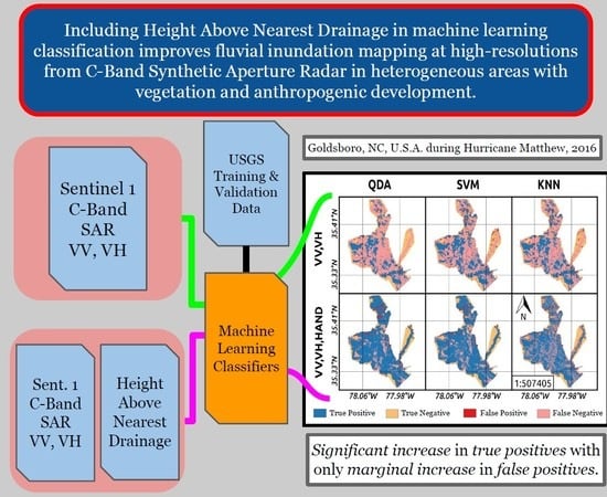
:Floods are one of the most wide-spread, frequent, and devastating natural disasters that continue to increase in frequency and intensity. Remote sensing, specifically synthetic aperture radar (SAR), has been widely used to detect surface water inundation to provide retrospective and near-real time (NRT) information due to its high-spatial resolution, self-illumination, and low atmospheric attenuation. However, the efficacy of flood inundation mapping with SAR is susceptible to reflections and scattering from a variety of factors including dense vegetation and urban areas. In this study, the topographic dataset Height Above Nearest Drainage (HAND) was investigated as a potential supplement to Sentinel-1A C-Band SAR along with supervised machine learning to improve the detection of inundation in heterogeneous areas. Three machine learning classifiers were trained on two sets of features dual-polarized SAR only and dual-polarized SAR along with HAND to map inundated areas. Three study sites along the Neuse River in North Carolina, USA during the record flood of Hurricane Matthew in October 2016 were selected. The binary classification analysis (inundated as positive vs. non-inundated as negative) revealed significant improvements when incorporating HAND in several metrics including classification accuracy (ACC) (+36.0%), critical success index (CSI) (+39.95%), true positive rate (TPR) (+42.02%), and negative predictive value (NPV) (+17.26%). A marginal change of +0.15% was seen for positive predictive value (PPV), but true negative rate (TNR) fell −14.4%. By incorporating HAND, a significant number of areas with high SAR backscatter but low HAND values were detected as inundated which increased true positives. This in turn also increased the false positives detected but to a lesser extent as evident in the metrics. This study demonstrates that HAND could be considered a valuable feature to enhance SAR flood inundation mapping especially in areas with heterogeneous land covers with dense vegetation that interfere with SAR.
1. Introduction
According to the World Disasters Report, flooding has affected over 830 million people, caused over 342 billion US dollars in damages, and led to over 57 thousand fatalities globally from 2006 to 2015 [1]. Moreover, flooding is expected to play a growing role in the future as the number of flood prone people, impacted cropland, and overall flood risk is expected to increase by the year 2050 according to a study that used 21 different climate models to simulate conditions [2].
Having more accurate and reliable flood inundation information on both retrospective and near real-time (NRT) (within 24 h) flood events could be a major asset to flood forecasters, public officials, first responders, and the general public. These stakeholders could leverage this information for a variety of applications including model validation, insurance underwriting, risk management, NRT evacuation mapping, and emergency response routing. Flood modelers use retrospective data to calibrate and validate their models while insurance and risk managers could use historical flood inundation data to estimate future risk and trends. Therefore, having more information on the spatial extents of inundation would be of great value to a breadth of stakeholders.
Remote sensing has been utilized to provide flood inundation observations on a NRT, global scale basis. The Dartmouth Flood Observatory in cooperation with the National Aeronautics and Space Administration (NASA) delivers a daily flood product at a 250m spatial resolution derived from Moderate Resolution Imaging Spectroradiometer (MODIS) bands 1, 2, and 7 but is affected by a variety of factors including direct cloud cover, cloud, and terrain shadows, and volcanic material [3]. Another prominent platform includes the Global Flood Detection System (GFDS) that uses microwave instruments (36.5–37.0 GHz) from a variety of satellites including the NASA Earth Observing Satellite (EOS) Aqua (AMSR-E instrument), Global Change Observation Mission–Water (AMSR-2 instrument), and Global Precipitation Mission (GPM) [4]. GFDS provides fractional water coverage observations derived from brightness temperatures on daily time steps or less at low spatial resolutions of approximately 10km. This approach is much more resilient to cloud cover and shadow, but does incur the penalty of lower spatial resolution as well as the uncertainty associated with the calculated fractional water coverage value.
An alternative sensor is synthetic aperture radar (SAR) which has been widely used to detect surface water inundation [5,6,7,8]. SAR provides advantage over multi-spectral or passive microwave systems due to high-spatial resolution, self-illumination, and low atmospheric attenuation. The Sentinel-1 constellation from the European Space Agency (ESA) is one of the active, freely-available sources of SAR data currently available with high spatial resolutions and latencies of less than 1 h [9]. The temporal resolution of Sentinel-1 is 6 to 12 days which is comparable to other SAR sensors such as TerraSAR-X (11 days) and Radarsat-2 (24 days) [7]. The Sentinel-1 instruments operate at a C-Band (5.405 GHz) frequency with bandwidth of 100 MHz. The instruments operate in various modes but over land are typically limited to the Interferometric Wide (IW) mode capture with two polarizations, vertical transmit and vertical receive (VV) and vertical transmit and horizontal receive (VH) [9].
Detecting inundated areas with SAR is made possible by the properties of the SAR system. Sentinel-1 is a right side-looking system that transmits at incident angles of 20 to 46 degrees [9]. The backscatter or the portion of the reflected signal that is directed back towards the satellite is quantified to an accuracy of 1dB [9]. Smooth open surfaces, such as calm surface water, act as reflective planes that reduce backscatter. In contrast, land covers such as agricultural fields, forests, prairies, and anthropogenic developments can exhibit various types of scattering including surface, volume, double-bounce, and diffuse scattering due to the surface roughness of the targets. Scattering decreases specular reflectance and increases observed backscatter. This difference in backscatter can be leveraged by supervised machine learning methods to decide upon an optimal decision boundary that reduces misclassification errors for inundated mapping.
Detecting inundation for densely vegetated and urban areas with SAR remains a challenge due to corner reflection and diffuse scattering [4,5,7,10,11,12]. Additionally, flat urban surfaces such as roads exhibit similar reflection properties as urban surface water [6]. Differences between inundated and non-inundated backscatter over vegetated land covers of static spatial domains have been demonstrated in previous studies [10,11]. However, these backscatter differences are sensitive to changes in water depth, soil moisture, SAR sensor parameters, wavelengths, terrain, and vegetation properties. These factors tend to make accurate inundation mapping of heterogeneous regions difficult with exclusive use of SAR.
An assortment of methodologies has been developed to counter these aforementioned limitations in SAR based inundation mapping. Multi-temporal approaches are common since they establish temporal statistics particularly coherence that can be leveraged to detect newly flooded areas when compared to dry areas in previous imagery [12,13,14,15,16,17,18,19,20]. Other techniques take different approaches that seek to exploit the local spatial dependencies of flooded areas by utilizing texture-based or object-based approaches such as mathematical morphological operations to name an example [17,20,21,22]. A variety of flood indices have also been developed and used with remote sensing data to better generate thresholds for flood classification, including the normalized difference flood index and normalized difference flood in vegetated areas index [15,23]. The actual classification task explored by many studies involves single band thresholding [13,14,15,18] as opposed to a machine learning approach that is proposed in this study. Several techniques are proposed in the literature that target vegetated or urban areas specifically including one that identifies flooded buildings [14,19,20]. Ancillary data and bi-static approaches are also explored by some researchers including the use of land cover information and multi-sensor data sources [23,24,25]. The literature is rich with a collection of valid procedures that seek to add value to Earth observation datasets by producing higher skill flood inundation maps. For this purpose, this study investigates the utility of auxiliary data, specifically high-resolution (10 m) terrain information normalized to fluvial features, in conjunction with SAR and pixel-based, supervised machine learning for detecting inundated areas in heterogeneous regions that include high vegetation and anthropogenic development.
Data fusion is a technique that has been commonly used in remote sensing to merge a variety of datasets for the purpose of enhancing the consistency, accuracy, or utility of the stand-alone datasets. Available terrain information on global scale could be used to enhance inundation mapping. In this study, the application of a hydrologically relevant terrain index, the Height Above Nearest Drainage (HAND), that normalizes topography to the elevation of the nearest channel bottom along the relevant drainage line [26,27], is tested. HAND has been generated for the entire Continental United States (CONUS) at a 10 m spatial resolution (1/3 arc second) by using the existing United States Geological Survey (USGS) National Elevation Dataset (NED) as a DEM and the National Hydrography Dataset (NHD), and for flowlines and catchments [28]. HAND has been used for assisting remote sensing inundation mapping as a post-processing mask that eliminates areas of low inundation risk which was shown to be useful for reduction of commission errors [7,29]. HAND has also been used to assist the single band thresholding but further work is needed utilizing more advanced detection algorithms [30].
The study seeks to investigate the benefits of fusing HAND as a feature to Sentinel-1 SAR VV and VH dual pol observations to reduce both errors in commission and omission for the mapping of riverine flooding within regions with heterogeneous land covers. Three machine learning classification algorithms, Quadratic Discriminant Analysis (QDA), Support Vector Machine (SVM), and k-nearest neighbors (KNN), were compared for their abilities to derive complex decision boundaries between inundated and non-inundated dated. The two feature sets, VV and VH, and VV, VH, and HAND, and three classifiers were validated by five different classification metrics and examined for their performance across multiple land cover groups.
2. Materials and Methods
2.1. Study Areas
Three study areas were selected in eastern North Carolina (NC), United States that coincide with the communities of Smithfield, Goldsboro, and Kinston. All three sites lie along the Neuse River which stretches 443km from the Piedmont north of Durham, NC, to Pamlico Sound downstream of New Bern, NC, draining the Neuse River Basin (Accounting Unit: 030202) as seen in Figure 1 [31]. These study areas were selected not only for their temporal alignment with a Sentinel-1A observation but also for the availability of independent inundation data for a severe flood of record caused by Hurricane Matthew in October 2016. The Hurricane brought upon cumulative rainfall totals of 10.4 to 37.3 cm (4.1 to 14.7 in) from October 7 to the 9th across the Neuse River Basin [32]. The gentle and rolling terrain of the region, along with pine woodlands, floodplain forests, agricultural fields, and developed land covers, provide difficulties for SAR surface water detection that we sought to improve upon using the proposed methods. The study areas also contain a variety of other smaller water bodies and creeks that feed the Neuse River which provide additional hydrologic factors to consider. The independent validation dataset was furnished by a USGS report concerning flooding in North Carolina after Hurricane Matthew [32]. The flood inundation maps were developed using several tools including high water marks (HWM), USGS stream gages, and DEMs. The HWM were collected by documenting the location and elevation of high-water indicators shortly after the storm event. For each study area, a water surface raster was developed by interpolating these HWM along with the peak stage elevation recorded at the site’s USGS station. This flood inundation surface was then intersected with a DEM. The light detection and ranging (lidar) DEM was collected by the North Carolina Floodplain Mapping Program in 2016 with a spatial resolution of 0.9525 m, a vertical root mean square error of 18.2 cm, and a nominal point spacing of 0.07 m or better [32]. Areas that had a higher water surface elevation according to the water surface raster than the ground elevation according to the DEM were labeled as inundated and vice versa. Since the validation dataset was developed by an independent agency with in-situ measurements and intersected with a high-resolution DEM independent of the NED, this provides an excellent independent benchmark to compare the proposed methodology to.
Uncertainties in this dataset can be attributed to a number of factors including the collection of the HWM, the DEM, interpolation techniques, anthropogenic structures, the number of HWMs collected, regions with low density of HWM, extrapolation of HWM elevations, and hydrodynamic effects not considered [33]. Temporal alignment with SAR is also an issue since the three sites peaked at different times [34]. For the case of the Goldsboro study area, Quaker Neck Lake in the western portion of the site was not included in the USGS inundated area despite there being evidence from the SAR and from stock aerial imagery that the lake is perennially inundated. To counter this limitation, the Quaker Neck Lake was added to the inundation validation dataset, as seen in Figure 1c. Nevertheless, the availability of this information along with the challenges associated with the sites make this a good case study for examining how HAND and machine learning methods could be leveraged for improving SAR based inundation mapping. Additional information for each site is listed in Table 1.
2.2. Overview
Figure 2 provides a graphical overview of the methodology employed to test how HAND affects SAR based flood inundation mapping using machine learning. Input data were preprocessed and split into two feature sets (VV and VH, and VV, VH, and HAND) for three different study areas. Sample points were sampled from independently collected validation data to train three machine learning classifiers. The tuned models generated flood inundation map predictions for the three study sites which were then compared to the validation dataset using primary and secondary binary classification metrics. Land cover data was used for the analysis portion to better understand and interpret the results.
2.3. Features and Training Samples
A variety of geospatial datasets were used for this study including landcover, SAR observation, NHD Plus flowlines and watersheds, USGS flood inundation maps, and HAND. Open-source spatial data tools, including Geospatial Data Abstraction Library (GDAL) and Quantum Geographical Information System (QGIS), were used for projecting, merging, clipping, and plotting spatial data [35,36,37,38]. The projection used for this study on all geographic data was the Albers Conic Equal Area with the Geodetic Reference System 1980 (GRS80) spheroid in order to preserve areas [39]. All scripts employed are available online (see Appendix A).
The Sentinel-1A satellite provided a useful observation of the study areas during the Hurricane Matthew storm event that was acquired on 12 October, 2016 at 11:15 Coordinated Universal Time (UTC) (see Appendix A for product details). The Sentinel-1A product, dual polarized (VV and VH) observations were used and processed by European Space Agency (ESA) to the Level-1 ground range detected (GRD) product level, as well as georeferenced by projecting the slanted data onto the WGS84 Earth ellipsoid model [40]. The products are detected and multi-looked for reduced speckling that results in a HR image of approximately 10m for both range and azimuth directions [40]. This Sentinel-1A Level-1 GRD-HR observation of interest is presented as a Digital Numbers (DN) file with Ground Control Points (GCP) that requires additional preprocessing prior to classification. The ESA provides the Sentinel Application (SNAP) Toolbox that was used to calibrate into backscatter values, as well as speckle filter using the Refined Lee filter [41,42].
The HAND dataset required minimal preprocessing other than projecting, resampling, and aligning to the SAR dataset. While the HAND dataset was already at approximately the same spatial resolution of the SAR data, it was nevertheless resampled using bilinear interpolation for enhanced pixel alignment. This is illustrated as false color images in Figure 3 and as two-dimensional scatter plots in Figure 4. The three-dimensional scatter plots represent a random two percent sample of the data to reduce over-crowding and better convey the geometry. All SAR and HAND data presented in this paper are in decibels (dB) and meters, respectively.
For each study area, a random sample of 40 points were selected from the validation datasets for training the three machine learning classifiers (see Appendix A for DOI). The samples were balanced, meaning half were non-inundated and the other half were inundated.
2.4. Classification
In order to discriminate between inundated and non-inundated areas, supervised machine learning algorithms provide a means of classifying the study area given the available features and training data. There are a multitude of machine learning classifiers to choose from but three were selected for this study, QDA, SVM, and KNN, due to their previous usage in remote sensing applications [43,44,45,46,47]. Training sets sampled from the validation data were used to train all three models for both sets of features (VV and VH and VV, VH, and HAND) on each study site. Generalizing the models was completed with parallel computing to ensure fast and scalable predictions that could be applied to larger areas if needed. The training and classification times were benchmarked and averaged by algorithm across ten trials per feature set and study area combination. All trials were completed on a 64-bit machine with 4 cores each with 0.90 GHz and a total of 8 GB of available memory. Further details on each algorithm, metric, parameter tuning, and training samples are subsequently presented.
2.4.1. Quadratic Discriminant Analysis (QDA)
Of the available machine learning algorithms, QDA provides the benefits of simplicity due to the multivariate Gaussian assumptions. QDA utilizes training or sample data to determine the mean and covariance matrix of each class directly. Generalizing class membership is done by assuming the features for each class are of a multivariate Gaussian distribution (Yc ~ N(μc,Σc), where c represents the class). A likelihood ratio test, as seen in Equation (1), is utilized to find the most probable class for the given test point. For out of sample values, t values above 1 were assigned to the numerator’s class membership while the denominator’s class was assigned for values below 1. QDA differs from linear discriminant analysis (LDA) by assuming a separate covariance matrix for all the classes involved which adds to the number of parameters to be estimated thus potential favoring a reduced bias for increased variance [48]. By assuming a separate covariance matrix for each class, the decision boundary (or hypersurface) can be shown to be quadratic in nature [48].
2.4.2. Support Vector Machine (SVM)
Support Vector Machines (SVM) are supervised learning models that are used for two-class classification problems. Training a model is known as a learning problem because it seeks to minimize an objective function by tuning model parameters until the optimal values are obtained. SVMs seek to devise a hyper-plane that separates the two classes by maximizing the functional margin between the decision plane and the neighboring training data points. In the general case, maximizing this margin yields a lower misclassification rate when generalized to out of sample data. The SVM is mathematically described in the primal form as seen in Equation (2) [49].
where xi ∈ Rn, in two classes with a response vector y ∈ Rt such that yi ∈ {-1,1}. Φ(xi) maps xi into a higher dimensional space and C > 0 is the penalty parameter on the error term of the objective function. Solving for the Lagrangian dual of the primal problem in equation 2 yields a streamlined optimization problem illustrated in Equation (3) [49].
where C > 0 is the upper bound and Q is an l x l positive semidefinite matrix such that Qij = yiyjK(xi,xj) = yiyjϕ(xi)Tϕ(xj). The K(xi,xj) = ϕ(xi)Tϕ(xj) function represents the kernel function which maps the data into higher dimensional space. In the case of this experiment, a radial basis function (RBF) meaning K(xi,xj) = exp(γ||xi-xj||2), γ >0 was used as the kernel function. While the gamma parameter in the RBF kernel does require tuning, it has the added benefit of allowing the SVM to form non-linear decision boundaries that may better represent the optimal decision boundary especially if the data is non-linear in nature.
The tuning of the penalty, C, and gamma, γ, parameters, involved using a grid search 10-fold cross validation (CV). For the grid search, every combination of values of C and γ from 0.02 to 1 spaced at intervals of 0.02 were selected. The CV procedure sought to find the optimal setting for the two parameters by splitting the training data into k equally sized sets. For each fold, 9 out of the 10 folds were used for training the SVM and a misclassification rate was determined for the remaining fold. The 10 misclassification error rates were averaged for the given parameter values and the optimal settings were determined to be the combination that minimized the misclassification rate.
2.4.3. K-Nearest Neighbors (KNN)
KNN represents one of the simplest classification techniques available. For each point, the k-nearest neighbors based on Euclidean distance are determined, which requires distance calculations between every point and every other point. Among these k-nearest neighbors, the class label of the majority is selected to be the class label of the point in question. The proportion of k-nearest neighbors with each class label corresponds to the probability of the point belonging to one of those classes, as shown in Equation (4) [49].
with Ω0 being the set of k-nearest neighbors. For example, three nearest neighbors of a data point are determined to have class labels of inundated, inundated, and non-inundated. Since 2 out of 3 points are labeled to be inundated, then the corresponding probability that the point is inundated is 0.667 and hence classified as inundated. This algorithm develops very complex and scattered decision boundaries that may or may not work for specific datasets. KNN suffers from the curse of dimensionality for higher dimensionality datasets but is not of concern for this experiment due to the low dimensional feature sets tested (2 and 3).
The selection of the k parameter was done by a parameter sweep of k values from 1 to 25 with 10-fold cross validation. As in the tuning of the SVM, CV determined the error rate for each value of k for each of the ten folds in the data. The optimal selection of k for each feature set and study area was determined individually by minimizing this out of sample error rate.
2.5. Performance Metrics
Due to the two-class predictions required for flood mapping, binary classification statistics were calculated for each study area. Inundated (I) was taken as the positive condition and non-inundated (NI) was regarded as the negative condition. The primary metrics included true positives (TP), true negatives (TN), false positives (FP), and false negatives (FN). These in turn were used to calculate the secondary metrics including positive predictive value (PPV), negative predictive value (NPV), true positive rate (TPR), true negative rate (TNR), critical success index (CSI), and overall accuracy (ACC). TPR, together with TNR, are specific terms for components of producer’s accuracies which is the accuracy of the dataset given the producer’s point of view. ACC aggregates TPR and TNR equally while weighing for the area of observed I and NI. It does not make a distinction between the relative cost of FN and FP. Alternatively, PPV and NPV are terms for the two components of user’s accuracy which could also be viewed as the probability of correct labeling given a predicted dataset. For example, if the producer’s accuracy for inundated (PPV) corresponds to 0.85 then 85% of the inundated pixels for that dataset are actually inundated in the reference dataset. A summary of these metrics, their descriptions, and formulas are listed in Table 2.
The previously listed metrics were also determined on a per landcover (LC) group basis to examine how the results from the proposed methods are affected by different LC types. Landcover data was obtained for post-classification analysis from the National Land Cover Database (NLCD) at a spatial resolution of 30m [50,51]. The classification system for the NLCD2011, based on a modified version of the Anderson Land Cover Classification System, contains 8 level I land cover classes and 20 level II sub-classes [50,51,52]. Overall, the selected study areas contain 15 of the 20 sub-classes with the top three prevalent sub-classes being woody wetlands, cultivated-crops, and developed open-space. The remaining 5 sub-classes are not relevant because 4 of them are unique to Alaska, the fifth being perennial ice/snow. To simplify the analysis, the level-II sub-classes were aggregated into three land cover groups of interest including developed, canopy, and agriculture. Developed contained all the developed level-II land covers, while canopy included all the forest land covers as well as the shrub/scrub and woody wetlands. Agriculture included both land covers in the planted/cultivated level I land covers. Lastly, the 30 m dataset was down-sampled and pixel aligned to match the native SAR spatial resolution of 10m by means of nearest-neighbor interpolation due to the categorical nature of the landcover dataset. Descriptive statistics including fractional coverage and km2 by LC group and by study site are detailed in Table 3. Each study site, Smithfield, Goldsboro, and Kinston, contains approximately 195.7E3, 747.4E3, 278.8E3, and samples (pixels), respectively, for a total of 1221.9E3 samples. The spatial distribution of the land cover groups is illustrated in Figure 5.
3. Results
3.1. Primary Metrics
The results for the primary metrics in number of pixels (in 1000’s) utilized in this experiment are presented in Table 4 for both feature sets for all three study areas and models aggregated together. On an overall basis, both feature sets under predict the inundated areas. For VV and VH, and VV, VH, and HAND, the number of inundated pixels in thousands predicted were 292.2 and 599.3, respectively, compared to 702.5 inundated in the validation. This under prediction can be better explained by the Euclidean geometry of the data and the decision boundaries generated by the classifiers which will be discussed later but simply introduced here. By integrating HAND into the prediction, a sizeable improvement was seen in the area of correctly predicted inundation (from 279.9 to 575 thousand pixels). Inverse to this improvement, an increase in falsely predicted non-inundation (FP) was also witnessed by integrating HAND into the feature set which increased from 12.3 to 24.3 thousand pixels. Overall, the increase in FP (12E3 pixels) is significantly less than the decrease in FN (295.1E3 pixels). This trade-off is also seen in the values for the secondary metrics, as seen later in the results.
Figure 6 shows how the primary metrics are spatially distributed across the study areas, classifiers, and feature sets. Sizeable improvements in true positives are evident by the increase in blue areas for all three study areas and classifiers. The increase in blue areas came also at the expense of the increase in a few red areas or false positives. Less variability is seen across the models when compared to the change that is seen by expanding the feature set with HAND. A rough texture is witnessed for the KNN results for the three features across the three study areas, which will be further explored later on.
3.2. Secondary Metrics
For most of the five secondary metrics considered, a considerable improvement was seen across feature sets for the different models and study areas as shown in Figure 7. Overall, ACC, CSI, TPR, and NPV saw the largest improvements of 44.7% to 80.7%, 39.2% to 79.1%, 39.8% to 81.9%, and 14.4% to 31.7%, respectively. A very marginal improvement of 95.8% to 95.9% was seen for PPV while TNR fell from 85.3% to 70.8%. The drop is associated with a reduction of TN and the complementary increase of FP which was seen across classifiers and study areas. On an overall basis for the VV, VH, HAND feature set, QDA, and SVM outperformed the KNN classifier.
Comparing the change in secondary metrics across LC by adding HAND as a feature in Figure 8 illustrates a large improvement for ACC on canopy, developed, and agriculture LC groups of 59.0%, 21.1%, and 8.7%, respectively. A sizeable improvement in TPR was also seen for canopy, developed, and agriculture of 71.2%, 41.1%, and 19.6%, respectively. CSI went up for canopy 68.0%, developed 34.7%, and agriculture 13.7%. Improvements for the three LC groups were also seen in the same relative order for the NPV metric but not for PPV which had little change for canopy and slight decrease for agriculture. TNR fell for canopy, agriculture, and developed LCs by margins of 26.6%, 15.8%, 8.0%, respectively.
3.3. Decision Boundaries
Plotting a randomly selection (≤ 0.2%) of the individual points and the resulting primary metric label for the Goldsboro study area in Figure 9 and Figure 10 illustrates the nature of the decision boundaries generated by the three classifiers employed and the relationship between HAND and VV or VH backscatter. Figure 9 illustrates the boundaries for the VV and VH feature set, while Figure 10 shows the boundaries for the VV, VH, and HAND feature set. Since TP and FP correspond to predicted inundation and TN and FN correspond to predicted non-inundation, the boundary between the two groups aligns with the decision boundary roughly speaking. The SAR only feature sets show decision boundaries that are near vertical, which is expected since HAND is not considered in the training. Incorporating HAND changes the nature of the boundaries to vary across the HAND axis as well. For all three classifiers in the HAND feature set, the decision boundaries tend decrease in HAND values as the backscatter values increase but the trend levels out or begins to increase again as the backscatters continue to increase. This creates an upwardly concave decision boundary. The decision boundaries for QDA and SVM are much more evident and abrupt than the decision boundary for KNN. This is due to the properties of QDA and SVM as discussed in the methodology where QDA develops a quadratic boundary and SVM with a radial basis kernel generates a non-linear boundary that maximizes the margin between classes. KNN creates more local boundaries determined by local relative densities of points, which results in more irregular boundaries, which is also seen in the spatial results in Figure 5.
The predicted inundation and non-inundation follow expected trends for both feature sets. The predicted non-inundated conditions, TN and FN, represent higher backscatter and HAND values than the predicted inundated conditions, TP and FP. This relationship while expected is now better quantified by this study. The higher backscatter values (>−15 VV dB and >−20 dB for VH) have a larger spread of HAND values than lower backscatter values. By incorporating HAND, the decision boundary adjusts to capture more of the higher backscatter and low points which reduces FN to a greater extent than the increase in FP.
3.4. Training and Classification Performance Times
All training and classification functionality were clocked and averaged by algorithm across each study site and feature set combination with ten trials per combination. The mean and standard deviation of the times in seconds are presented in Table 5.
4. Discussion
The main objective of the study was to explore how incorporating HAND as a feature for flood inundation mapping can improve the quality of prediction across heterogeneous areas. Machine learning algorithms were used to explore the decision boundaries and minimize the misclassification errors that single band or single variable thresholding does not accurately capture. Overall, an increase in classification accuracies was observed by considering HAND into the feature set. A variety of other metrics including TPR, PPV, and NPV also improved. HAND data which is vertical elevation relative to the nearest relevant bottom drainage elevation helps classifiers detect inundated areas with higher backscatter values that may come from inundated vegetation or urban areas. Areas of dense vegetation and anthropogenic features saw better performance improvements than areas that associate with lower SAR backscatter. By including this feature, a penalty is paid by over-predicting on some of the higher backscatter/low HAND areas resulting in more FP and a lower TNR. The relative decrease in TN is less than the increase of FP and the increase of TPR which results in higher overall ACC and CSI values which was evident in Figure 9 and Figure 10. These trends were fairly consistent across the study areas and classifiers. Weather forecasting typically involves some level of wet bias which historically would favor FP to FN due to the inherent danger in under predicting impactful phenomena [53].
The three classifiers all responded to the change in feature sets slightly differently due to the nature of algorithms and how they generate decision boundaries. The relationship between HAND and SAR for the study areas were as expected with a higher density of inundated areas occurring for low HAND and backscatter regions. The variability in HAND values is higher for higher backscatter regions which is influenced by the role of vegetation and anthropogenic land covers. The variability of backscatter and HAND values associated with inundated and non-inundated areas in high backscatter/lower HAND areas still present an issue for detecting inundation which is improved upon by integrating HAND but some false detection still exists.
Comparing the performance of the individual classifiers shows that both QDA and SVM outperformed KNN for the VV, VH, HAND feature set on a majority of the metrics including ACC and CSI. This shows evidence that these maybe better suited to make higher skill maps possibly for their clear concave decision boundaries that are evident in Figure 10. In an operational setting, one must consider skill and computational costs so considering KNN as a classifier for low impact inundation maybe a wise choice while utilizing the most accurate classifiers, such as SVM or QDA for higher impact inundation events.
The proposed methodology has a number of limitations and sources of error. Integrating HAND into supervised learning algorithms limits to areas with validation data for proper tuning and application. The study compared three study areas with limited extents in the SAR’s range direction which limits the incidence angles and the resulting backscatter profiles. The limited extents also affect how HAND can be used to predict inundation since inundated HAND values will experience greater variation across larger scales. HAND is inherently connected to river networks, so its use is limited to fluvial events with limited to no utility in pluvial or coastal flooding. Additionally, within these local study areas, each stream reach has its own catchment and associated HAND value that determines inundation [26,27]. Utilizing one parameterized model across all catchments may have led to the increase TN in lower HAND and higher backscatter areas, since stream flows and the associated HAND threshold will vary across stream orders. Sources of error in the HAND dataset that is derived from the NED may also affect the efficacy of the prediction. Using the most accurate DEM’s available for HAND raster generation such as those from Lidar could provide an improvement. Lastly, temporal alignment is also another source of error since the Smithfield and Kinston sites did not align perfectly with the SAR image capture. This was most evident in the lower metrics for those sites in the SAR only feature set since HAND weighs significantly in the other feature set. Since this error was not adequately detected in the results, as seen in Figure 7, it is possible that other sources contributed more. Additional analysis was completed to see how terrain correction using SNAP affected the study but the results were largely unchanged for these flood events. Further work should be done to analyze the sources of variation and error in this methodology.
Future work on improving C-Band SAR for flood inundation mapping in heterogeneous areas could concentrate on generating unsupervised machine learning approaches to detecting inundation with HAND in order to automate the procedure for operational applications. HAND values should be applied in a catchment or near catchment level to avoid over predicting in certain areas. Other platforms for SAR or multi-spectral systems could also be investigated for integration with HAND for this application. Land cover information was used exclusively for analysis but could possibly be used to help cluster data prior to classification to discriminate between inundated and non-inundated areas of similar scattering properties. Exploiting spatial and temporal patterns should also be explored within the framework of this study as proposed by others [17,20,21,22]. Thinking beyond the production of binary inundation maps, this method could be integrated into the production of flood depth maps utilizing existing methods that estimate flood depths from remote sensing generated inundation maps [54,55].
5. Conclusions
This study has demonstrated how incorporating an auxiliary dataset, Height Above Nearest Drainage (HAND), to Sentinel-1 C-Band synthetic aperture radar (SAR) dual-polarized flood inundation predictions could significantly improve upon SAR-only flood inundation mapping in heterogeneous areas with dense vegetation and anthropogenic development. Three study areas in eastern North Carolina during the record floods of Hurricane Matthew were selected and United States Geological Survey (USGS) generated inundation maps were used as training and validation labels for three supervised machine learning classifiers, quadratic discriminant analysis (QDA), support vector machines (SVM), and k-nearest neighbor (KNN). These classifiers are trained and tuned to select optimal decision boundaries that can minimize misclassification errors when multiple features are included for prediction. Taking inundation as the positive condition, a variety of binary classification metrics including accuracy, critical success index, true positive rate, and negative predictive value showed improvements by integrating HAND into the feature set of 44.7% to 80.7%, 39.2% to 79.1%, 39.8% to 81.9%, and 14.4% to 31.7%, respectively. Positive predictive value showed a marginal change of 95.8% to 95.9% while true negative rate (TNR) fell from to 85.3% to 70.8% across classifiers, study areas, and land cover groups. This reduction in TNR is associated with an increase in false positives (FP) and corresponding decrease in true negatives (TN) due to the modification of the decision boundaries observed when incorporating HAND with VV and VH. Lower HAND and higher backscatter values are labeled as inundated where those values are not captured as inundation with prediction using the SAR only feature set. This causes some of those values to be mis-labeled but the increase in true positives (TP) more than offsets the drop in TN to increase overall accuracies. Future work should emphasize unsupervised learning approaches for automated procedures applied to larger areas that leverage HAND for enhanced flood inundation mapping using C-band SAR [17,22]. Consideration should be given to local HAND values to explore how this can improve classification metrics overall.
Author Contributions
Conceptualization, F.A. and J.J.; Data curation, F.A. and A.M.-H.; Formal analysis, F.A. and J.J.; Funding acquisition, F.A. and J.J.; Investigation, F.A.; Methodology, F.A. and J.J.; Project administration, F.A. and J.J.; Resources, F.A. and J.J.; Software, F.A., J.J. and A.M.-H.; Supervision, J.J.; Validation, F.A. and J.J.; Visualization, F.A. and J.J.; Writing – original draft, F.A. and J.J.; Writing – review and editing, F.A. and J.J. All authors have read and agreed to the published version of the manuscript.
Funding
This research has been funded by the University of Florida’s Graduate Research Fellowship as well as the support of the National Water Center (NWC) in Tuscaloosa, Alabama, USA. The National Water Center is part of the National Oceanic and Atmospheric Administration’s (NOAA) Office of Water Prediction (OWP).
Acknowledgments
Technical support for data processing was received from Donald Johnson and Fernando Salas of the NWC. Marie Peppler from the USGS provided support for data availability.
Conflicts of Interest
The authors declare no conflict of interest. The funders had no role in the design of the study; in the collection, analyses, or interpretation of data; in the writing of the manuscript, or in the decision to publish the results.
Appendix A
Sentinel-1 Product used: “S1A_IW_GRDH_1SDV_20161012T111514_20161012T111543_013456_01580C_1783.SAFE”. For more information, please see link for an explanation on the naming conventions (https://sentinel.esa.int/web/sentinel/user-guides/sentinel-1-sar/naming-conventions).
Training Samples and Scripts Used: Aristizabal, F. (2019). Flood Inundation Mapping Utilizing Synthetic Aperture Radar and Ancillary Data, HydroShare, http://www.hydroshare.org/resource/b35f259d7e754792ae5c266954fcabec.
References
- Sanderson, D.; Anshu, S. Resilience: Saving Lives Today, Investing for Tomorrow; World Disasters Report 2016; International Federation of Red Cross and Red Crescent Societies: Geneva, Switzerland, 2016. [Google Scholar]
- Nigro, J.; Slayback, D.; Policelli, F.; Brakenridge, G.R. NASA/DFO MODIS Near Real-Time (NRT) Global Flood Mapping Product Evaluation of Flood and Permanent Water Detection. Available online: https://floodmap.modaps.eosdis.nasa.gov//documents/NASAGlobalNRTEvaluationSummary_v4.pdf (accessed on 14 October 2014).
- De Groeve, T.; Brakenridge, G.R.; Paris, S. Global Flood Detection System Data Product Specifications; Joint Research Centre: Brussels, Belgium, 2015. [Google Scholar]
- Martinis, S. Automatic Near Real-Time Flood Detection in High Resolution X-Band Synthetic Aperture Radar Satellite Data Using Context-Based Classification on Irregular Graphs. Ph.D. Thesis, LMU, Munich, Germany, 2010. [Google Scholar]
- Kudahetty, C. Flood Mapping Using Synthetic Aperture Radar in the Kelani Ganga and the Bolgoda Basins, Sri Lanka; University of Twente Faculty of Geo-Information and Earth Observation (ITC): Enschede, the Netherlands, 2012. [Google Scholar]
- Stefan, S.; Matgen, P.; Hollaus, M.; Wagner, W. Flood detection from multi-temporal SAR data using harmonic analysis and change detection. Int. J. Appl. Earth Obs. Geoinf. 2015, 38, 15–24. [Google Scholar]
- Saatchi, S. SAR Methods for Mapping and Monitoring Forest Biomass. In SAR Handbook: Comprehensive Methodologies for Forest Mapping and Biomass Estimation; Flores, A., Herndon, K., Thapa, R., Cherrington, E., Eds.; in review; NASA: Washingtong, DC, USA, 2020. [Google Scholar]
- Yukihiro, S.; Rangoonwala, A.; Elijah, W.R., III. Monitoring Coastal Inundation with Synthetic Aperture Radar Satellite Data; No. 2011-1208; US Geological Survey: Reston, VI, USA, 2011.
- SENTINEL-1 SAR User Guide, ESA. Available online: https://sentinel.esa.int/web/sentinel/user-guides/sentinel-1-sar (accessed on 1 January 2019).
- Kasischke, S.E.; Smith, K.B.; Bourgeau-Chavez, L.L.; Romanowicz, E.A.; Brunzell, S.; Richardson, C.J. Effects of seasonal hydrologic patterns in south Florida wetlands on radar backscatter measured from ERS-2 SAR imagery. Remote Sens. Environ. 2003, 88, 423–441. [Google Scholar] [CrossRef]
- Hess, L.L.; Melack, J.M.; Novo, E.M.L.M.; Barbosa, C.C.F.; Gastil, M. Dual-season mapping of wetland inundation and vegetation for the central Amazon basin. Remote Sens. Environ. 2003, 87, 404–428. [Google Scholar] [CrossRef]
- Julie, B.; Rapinel, S.; Corgne, S.; Pottier, E.; Hubert-Moy, L. TerraSAR-X dual-pol time-series for mapping of wetland vegetation. ISPRS J. Photogramm. Remote Sens. 2015, 107, 90–98. [Google Scholar]
- Cécile, C.; Rapinel, S.; Frison, Pi.; Bonis, A.; Mercier, G.; Mallet, C.; Corgne, S.; Rudant, J. Mapping and characterization of hydrological dynamics in a coastal marsh using high temporal resolution Sentinel-1A images. Remote Sens. 2016, 8, 570. [Google Scholar]
- Marco, C.; Pelich, R.; Pulvirenti, L.; Pierdicca, N.; Hostache, R.; Matgen, P. Sentinel-1 InSAR coherence to detect floodwater in urban areas: Houston and Hurricane Harvey as a test case. Remote Sens. 2019, 11, 107. [Google Scholar]
- Fabio, C.; Marconcini, M.; Ceccato, P. Normalized Difference Flood Index for rapid flood mapping: Taking advantage of EO big data. Remote Sens. Environ. 2018, 209, 712–730. [Google Scholar]
- Jean-Michel, M.; Le Toan, T. Mapping of flood dynamics and spatial distribution of vegetation in the Amazon floodplain using multitemporal SAR data. Remote Sens. Environ. 2007, 108, 209–223. [Google Scholar]
- Sandro, M.; Twele, A. A hierarchical spatio-temporal Markov model for improved flood mapping using multi-temporal X-band SAR data. Remote Sens. 2010, 2, 2240–2258. [Google Scholar]
- Pulvirenti, L.; Chini, M.; Pierdicca, N.; Guerriero, L.; Ferrazzoli, P. Flood monitoring using multi-temporal COSMO-SkyMed data: Image segmentation and signature interpretation. Remote Sens. Environ. 2011, 115, 990–1002. [Google Scholar] [CrossRef]
- Luca, P.; Pierdicca, N.; Chini, M.; Guerriero, L. Monitoring flood evolution in vegetated areas using COSMO-SkyMed data: The Tuscany 2009 case study. IEEE J. Sel. Top. Appl. Earth Obs. Remote Sens. 2013, 6, 1807–1816. [Google Scholar]
- Viktoriya, T.; Martinis, S.; Marzahn, P.; Ludwig, R. Detection of temporary flooded vegetation using Sentinel-1 time series data. Remote Sens. 2018, 10, 1286. [Google Scholar]
- Antara, D.; Grimaldi, S.; Ramsankaran, R.A.A.J.; Pauwels, V.R.N.; Walker, J.P. Towards operational SAR-based flood mapping using neuro-fuzzy texture-based approaches. Remote Sens. Environ. 2018, 215, 313–329. [Google Scholar]
- Simon, P.; Jüssi, M.; Martinis, S.; Twele, A. Mapping of flooded vegetation by means of polarimetric Sentinel-1 and ALOS-2/PALSAR-2 imagery. Int. J. Remote Sens. 2017, 38, 3831–3850. [Google Scholar]
- Ward, D.P.; Petty, A.; Setterfield, S.A.; Douglas, M.M.; Ferdinands, K.; Hamilton, S.K.; Phinn, S. Floodplain inundation and vegetation dynamics in the Alligator Rivers region (Kakadu) of northern Australia assessed using optical and radar remote sensing. Remote Sens. Environ. 2014, 147, 43–55. [Google Scholar] [CrossRef]
- Chayma, C.; Chini, M.; Abdelfattah, R.; Hostache, R.; Chokmani, K. Flood mapping in a complex environment using bistatic TanDEM-X/TerraSAR-X InSAR coherence. Remote Sens. 2018, 10, 1873. [Google Scholar]
- Stefania, G.; Xu, J.; Li, Y.; Pauwels, V.R.N.; Walker, J.P. Flood mapping under vegetation using single SAR acquisitions. Remote Sens. Environ. 2020, 237, 111582. [Google Scholar]
- Donato, N.A.; Cuartas, L.A.; Hodnett, M.; Rennó, C.D.; Rodrigues, G.; Silveira, A.; Waterloo, M.; Saleska, S. Height Above the Nearest Drainage–a hydrologically relevant new terrain model. J. Hydrol. 2011, 404, 13–29. [Google Scholar]
- Daleles, R.C.; Nobre, A.D.; Cuartas, L.A.; Soares, J.V.; Hodnett, M.G.; Tomasella, J.; Waterloo, M.J. HAND, a new terrain descriptor using SRTM-DEM: Mapping terra-firme rainforest environments in Amazonia. Remote Sens. Environ. 2008, 112, 3469–3481. [Google Scholar]
- Liu, Y.Y.; Maidment, D.R.; Tarboton, D.G.; Zheng, X.; Wang, S. A CyberGIS integration and computation framework for high-resolution continental-scale flood inundation mapping. JAWRA J. Am. Water Resour. Assoc. 2018, 54, 770–784. [Google Scholar] [CrossRef] [Green Version]
- André, T.; Cao, W.; Plank, S.; Martinis, S. Sentinel-1-based flood mapping: A fully automated processing chain. Int. J. Remote Sens. 2016, 37, 2990–3004. [Google Scholar]
- Chang, H.; Nguyen, B.D.; Zhang, S.; Cao, S.; Wagner, W. A comparison of terrain indices toward their ability in assisting surface water mapping from Sentinel-1 data. ISPRS Int. J. Geo Inf. 2017, 6, 140. [Google Scholar]
- United States Geological Survey. Boundary Descriptions and Names of Regions, Subregions, Accounting Units and Cataloging Units. 2017. Available online: https://water.usgs.gov/GIS/huc_name.html (accessed on 1 January 2019).
- Musser, J.W.; Watson, K.M.; Gotvald, A.J. Characterization of Peak Streamflows and Flood Inundation at Selected Areas in North Carolina following Hurricane Matthew, October 2016; No. 2017-1047; US Geological Survey: Reston, VI, USA, 2017.
- North Carolina Floodplain Mapping Program. North Carolina’s Spatial Data Download: North Carolina Emergency Management Web Page. 2016. Available online: https://rmp.nc.gov/sdd/ (accessed on 5 December 2016).
- U.S. Geological Survey. National Water Information System Data Available on the World Wide Web (USGS Water Data for the Nation). 2016. Available online: http://waterdata.usgs.gov/nwis/ (accessed on 13 January 2019).
- QGIS Development Team. QGIS Geographic Information System. Open Source Geospatial Foundation. 2009. Available online: http://qgis.osgeo.org (accessed on 1 January 2019).
- R Core Team. R: A Language and Environment for Statistical Computing. R Foundation for Statistical Computing, Vienna, Austria. Available online: https://www.R-project.org/ (accessed on 1 January 2017).
- Roger, B.; Keitt, T.; Rowlingson, B. Rgdal: Bindings for the ‘Geospatial’ Data Abstraction Library. R Package Version 1.2-15. Available online: https://CRAN.R-project.org/package=rgdal (accessed on 1 January 2017).
- Geospatial Data Abstraction Library (GDAL). OSGEO Project. Open Source. 2017. Available online: http://www.gdal.org (accessed on 1 January 2017).
- ESRI: 102003. USA Contiguous Albers Equal Area Conic: ESRI Projection—Spatial Reference. Available online: http://spatialreference.org/ref/esri/102003/ (accessed on 29 May 2019).
- SENTINEL-1 SAR Technical Guide, ESA. Available online: https://sentinel.esa.int/web/sentinel/technical-guides/sentinel-1-sar (accessed on 1 January 2017).
- Sikiru, Y.A.; Liu, R.; Wu, S. SAR image despeckling using refined Lee filter. In Proceedings of the 7th International Conference on Intelligent Human-Machine Systems and Cybernetics, Hangzhou, China, 26–27 August 2015; Volume 2, pp. 260–265. [Google Scholar]
- Sentinel Application Platform (SNAP). European Space Agency (ESA). 2017. Available online: http://step.esa.int/main/toolboxes/snap/ (accessed on 1 January 2017).
- John, H.; Billor, N.; Anderson, N. Comparison of standard maximum likelihood classification and polytomous logistic regression used in remote sensing. Eur. J. Remote Sens. 2013, 46, 623–640. [Google Scholar]
- Hong, H.; Naghibi, S.A.; Dashtpagerdi, M.M.; Pourghasemi, H.R.; Chen, W. A comparative assessment between linear and quadratic discriminant analyses (LDA-QDA) with frequency ratio and weights-of-evidence models for forest fire susceptibility mapping in China. Arab. J. Geosci. 2017, 10, 167. [Google Scholar] [CrossRef]
- Giorgos, M.; Im, J.; Ogole, C. Support vector machines in remote sensing: A review. ISPRS J. Photogramm. Remote Sens. 2011, 66, 247–259. [Google Scholar]
- Hector, F.-L.; Ek, A.R.; Bauer, M.E. Estimation and mapping of forest stand density, volume, and cover type using the k-nearest neighbors method. Remote Sens. Environ. 2001, 77, 251–274. [Google Scholar]
- Li, Y.; Cheng, B. An improved k-nearest neighbor algorithm and its application to high resolution remote sensing image classification. In Proceedings of the 17th International Conference on Geoinformatics, Fairfax, VA, USA, 12–14 August 2009; pp. 1–4. [Google Scholar]
- James, G. An Introduction to Statistical Learning: With Applications in R; Springer Verlag: Berlin, Germany, 2010. [Google Scholar]
- Chang, C.-C.; Lin, C.-J. LIBSVM: A library for support vector machines. ACM Trans. Intell. Syst. Technol. Tist 2011, 2, 27. [Google Scholar] [CrossRef]
- Collin, H.; Dewitz, J.; Yang, L.; Jin, S.; Danielson, P.; Xian, G.; Coulston, J.; Herold, N.; Wickham, J.; Megown, K. Completion of the 2011 National Land Cover Database for the conterminous United States–representing a decade of land cover change information. Photogramm. Eng. Remote Sens. 2015, 81, 345–354. [Google Scholar]
- National Land Cover Database (NLCD). United States Geological Survey (USGS). Multi-Resolution Land Characteristics (MRLC) Consortium. 2017. Available online: https://nationalmap.gov/landcover.html (accessed on 1 January 2017).
- Richard, A.J. A Land Use and Land Cover Classification System for Use with Remote Sensor Data; US Government Printing Office: Washinton, DC, USA, 1976; Volume 964.
- Eric, B.J.; Kim, S.D. Verification of the weather channel probability of precipitation forecasts. Mon. Weather Rev. 2008, 136, 4867–4881. [Google Scholar]
- Sagy, C.; Brakenridge, G.R.; Kettner, A.; Bates, B.; Nelson, J.; McDonald, R.; Huang, Y.; Munasinghe, D.; Zhang, J. Estimating floodwater depths from flood inundation maps and topography. JAWRA J. Am. Water Resour. Assoc. 2018, 54, 847–858. [Google Scholar]
- Anna, S.; Radice, A.; Molinari, D. A New Tool to Estimate Inundation Depths by Spatial Interpolation (RAPIDE): Design, Application and Impact on Quantitative Assessment of Flood Damages. Water 2018, 10, 1805. [Google Scholar]
Figure 1.
Neuse River Basin located within North Carolina (a) containing the three study sites Smithfield (b), Goldsboro (c), and Kinston (d). Each study site illustrates the high-water marks (HWM) collected by the United States geological survey (USGS), as well as the location of the USGS station. These data points were used to create the inundated areas within the study area boundaries.


Figure 2.
Methodology overview for study.

Figure 3.
False color red, blue, and green (RGB) images representing vertical transmit (VV), vertical receive (VH), and height above nearest drainage (HAND), respectively, for the three study areas in (a), (b), and (c).
Figure 3.
False color red, blue, and green (RGB) images representing vertical transmit (VV), vertical receive (VH), and height above nearest drainage (HAND), respectively, for the three study areas in (a), (b), and (c).


Figure 4.
Three-dimensional scatter plots representing a 2% random sample of the feature set data for the three study areas Smithfield (top row), Goldsboro (middle row), and Kinston (bottom row). Plotting limits were set to −25 to 0 dB for VV and VH while HAND plotting limits were 0 to 25 m. Labels were set using the class from the validation dataset.

Figure 5.
Illustrate the aggregation of the NLCD into one of three groups of interest including developed, canopy, and agriculture. All three study sites, Smithfield (a), Goldsboro (b), and Kinston (c), are shown.
Figure 5.
Illustrate the aggregation of the NLCD into one of three groups of interest including developed, canopy, and agriculture. All three study sites, Smithfield (a), Goldsboro (b), and Kinston (c), are shown.


Figure 6.
Spatial distribution of primary metrics, true positives (TP), false positives (FP), true negatives (TN), and false negatives (FN), for the two feature sets, three study areas, and three classifiers.
Figure 6.
Spatial distribution of primary metrics, true positives (TP), false positives (FP), true negatives (TN), and false negatives (FN), for the two feature sets, three study areas, and three classifiers.

Figure 7.
The average performance across classifiers on secondary metrics shown as the bar with the performance of each classifier shown in points. The metrics are grouped by feature set and then by study area. The overall results illustrate the metrics aggregated across all three study areas.
Figure 7.
The average performance across classifiers on secondary metrics shown as the bar with the performance of each classifier shown in points. The metrics are grouped by feature set and then by study area. The overall results illustrate the metrics aggregated across all three study areas.

Figure 8.
Changes in metrics across feature sets (VV, VH, and HAND minus VV and VH) for the three land cover groups listed by model and the average of the three models.
Figure 8.
Changes in metrics across feature sets (VV, VH, and HAND minus VV and VH) for the three land cover groups listed by model and the average of the three models.

Figure 9.
Primary metrics for all three classifiers on Goldsboro illustrated as scatter points for HAND vs. VV and HAND vs. VH for the feature set that did not include HAND. Demonstrates the decision boundaries generated by the classifiers and the relationship between SAR backscatter and HAND. Points are a random sample of overall study area (≤ 0.2%).

Figure 10.
Primary metrics for all three classifiers on Goldsboro illustrated as scatter points for HAND vs. VV and HAND vs. VH for the feature set that included HAND. Demonstrates the decision boundaries generated by the classifiers and the relationship between SAR backscatter and HAND. Points are a random sample of overall study area (≤ 0.2%).


Table 1.
Summary statistics and information for the three study areas with validation data furnished by the United States geological survey (USGS). Synthetic aperture radar (SAR). Observation occurred October 12th, 2016 at 11:15 UTC1 (06:15 EDT2).
Table 1.
Summary statistics and information for the three study areas with validation data furnished by the United States geological survey (USGS). Synthetic aperture radar (SAR). Observation occurred October 12th, 2016 at 11:15 UTC1 (06:15 EDT2).
| Site Name. | Area (km2) | USGS Station Number | Peak Date (MM/DD/YY) | Peak Gage Height (m) | SAR Observation Gage Height (m) | Prevalence3 |
|---|---|---|---|---|---|---|
| Smithfield | 21.8 | 02087570 | 10/09/16 | 8.87 | 5.83 | 0.798 |
| Goldsboro | 89.2 | 02089000 | 10/12/16 | 9.06 | 9.06 | 0.877 |
| Kinston | 28.8 | 02089500 | 10/14/16 | 8.63 | 6.98 | 0.620 |
| Total | 139.8 | Overall | 0.787 |
1 Coordinated Universal Time. 2 Eastern Daylight Time. 3 inundated fraction of study area.
Table 2.
Summary of primary and secondary binary classification metrics used.
| Name Formula | Definition |
|---|---|
| True Positive (TP) | Predicted I and observed I. |
| True Negative (TN) | Predicted NI and observed NI. |
| False Positive (FP) | Predicted I but observed NI. |
| False Negative (FN) | Predicted NI but observed I. |
| True Positive Rate (TPR) TP / (TP + FN) | Proportion of observed I areas predicted as I. |
| True Negative Rate (TNR) TN / (TN + FP) | Proportion of observed NI areas predicted as NI. |
| Positive Predictive Value (PPV) TP / (TP + FP) | Proportion of areas predicted as I correctly classified as I. |
| Negative Predictive Value (NPV) TN / (FN + TN) | Proportion of areas predicted as NI correctly classified as NI. |
| Critical Success Index (CSI) TP / (TP + FN + FP) | Proportion of areas observed I plus FN correctly classified as I. |
| Overall Accuracy (ACC) (TP + TN) / (TP + FN + FP + TN) | Proportion of all areas classified correctly. |
Table 3.
Sample size in pixels, fractional coverage, and areas (km2) for the three land cover groups of interest as well as the national land cover database (NLCD) Level II sub-classes used to define the land cover groups. The three study sites and the totals are listed for each.
Table 3.
Sample size in pixels, fractional coverage, and areas (km2) for the three land cover groups of interest as well as the national land cover database (NLCD) Level II sub-classes used to define the land cover groups. The three study sites and the totals are listed for each.
| Land Cover Group | Level II Classes | Fractional Coverage | Area (km2) | ||||||
|---|---|---|---|---|---|---|---|---|---|
| S1 | G2 | K3 | T4 | S1 | G2 | K3 | T4 | ||
| Developed | 21, 22, 23, 24 | 0.15 | 0.22 | 0.21 | 0.21 | 3.4 | 19.3 | 6.2 | 28.9 |
| Canopy | 41, 42, 43, 52, 90 | 0.45 | 0.34 | 0.51 | 0.40 | 9.7 | 30.5 | 14.7 | 55.0 |
| Agriculture | 81, 82 | 0.18 | 0.22 | 0.07 | 0.18 | 3.8 | 20.0 | 2.1 | 26.0 |
| Other | 11,12,31,51,71,72,73,74,95 | 0.22 | 0.22 | 0.20 | 0.21 | 4.8 | 19.5 | 5.7 | 30.0 |
| Totals By Site | 0.16 | 0.61 | 0.23 | 1.00 | 21.8 | 89.2 | 28.8 | 139.8 | |
1 Smithfield, 2 Goldsboro, 3 Kinston, 4 Totals by LC group.
Table 4.
Confusion matrix comparing primary metrics in pixels (1000’s) for both feature sets.
| Validation | |||||
|---|---|---|---|---|---|
| Non-Inundated | Inundated | Totals | |||
| Predicted | VV & VH | Non-Inundated | 71.1 | 422.6 | 493.7 |
| Inundated | 12.3 | 279.9 | 292.2 | ||
| VV, VH & HAND | Non-Inundated | 59.1 | 127.5 | 186.6 | |
| Inundated | 24.3 | 575 | 599.3 | ||
| Totals | 83.4 | 702.5 | 785.9 | ||
Table 5.
Mean and standard deviation of training and classification times (seconds) for each classification algorithm across each study site and feature set combination with ten trials per combination.
Table 5.
Mean and standard deviation of training and classification times (seconds) for each classification algorithm across each study site and feature set combination with ten trials per combination.
| Classification Algorithm | Classification + Training Time (seconds) | |
|---|---|---|
| Mean | Standard Deviation | |
| QDA | 3.92 | 1.59 |
| SVM | 3.21 | 1.22 |
| KNN | 1.22 | 0.54 |
© 2020 by the authors. Licensee MDPI, Basel, Switzerland. This article is an open access article distributed under the terms and conditions of the Creative Commons Attribution (CC BY) license (http://creativecommons.org/licenses/by/4.0/).
Share and Cite
MDPI and ACS Style
Aristizabal, F.; Judge, J.; Monsivais-Huertero, A. High-Resolution Inundation Mapping for Heterogeneous Land Covers with Synthetic Aperture Radar and Terrain Data. Remote Sens. 2020, 12, 900. https://doi.org/10.3390/rs12060900
AMA Style
Aristizabal F, Judge J, Monsivais-Huertero A. High-Resolution Inundation Mapping for Heterogeneous Land Covers with Synthetic Aperture Radar and Terrain Data. Remote Sensing. 2020; 12(6):900. https://doi.org/10.3390/rs12060900
Chicago/Turabian StyleAristizabal, Fernando, Jasmeet Judge, and Alejandro Monsivais-Huertero. 2020. "High-Resolution Inundation Mapping for Heterogeneous Land Covers with Synthetic Aperture Radar and Terrain Data" Remote Sensing 12, no. 6: 900. https://doi.org/10.3390/rs12060900
Note that from the first issue of 2016, this journal uses article numbers instead of page numbers. See further details here.