Urban Flood Mapping Using SAR Intensity and Interferometric Coherence via Bayesian Network Fusion

Abstract

Synthetic Aperture Radar (SAR) observations are widely used in emergency response for flood mapping and monitoring. However, the current operational services are mainly focused on flood in rural areas and flooded urban areas are less considered. In practice, urban flood mapping is challenging due to the complicated backscattering mechanisms in urban environments and in addition to SAR intensity other information is required. This paper introduces an unsupervised method for flood detection in urban areas by synergistically using SAR intensity and interferometric coherence under the Bayesian network fusion framework. It leverages multi-temporal intensity and coherence conjunctively to extract flood information of varying flooded landscapes. The proposed method is tested on the Houston (US) 2017 flood event with Sentinel-1 data and Joso (Japan) 2015 flood event with ALOS-2/PALSAR-2 data. The flood maps produced by the fusion of intensity and coherence and intensity alone are validated by comparison against high-resolution aerial photographs. The results show an overall accuracy of 94.5% (93.7%) and a kappa coefficient of 0.68 (0.60) for the Houston case, and an overall accuracy of 89.6% (86.0%) and a kappa coefficient of 0.72 (0.61) for the Joso case with the fusion of intensity and coherence (only intensity). The experiments demonstrate that coherence provides valuable information in addition to intensity in urban flood mapping and the proposed method could be a useful tool for urban flood mapping tasks.

1. Introduction

Flooding is a widespread and dramatic natural disaster that affects lives, infrastructures, economics and local ecosystems in the world. It is reported that flood events were the main cause of internal displacement in 2008 to 2015 [1,2], and global economic losses due to floods in economically strong and populated areas are projected to reach US $597 billion in 2016–2035 [3]. Remote sensing data can offer a synoptic view over large areas systematically and provides useful information about the extent and dynamics of floods. Several international initiatives such as the International Charter “Space and Major Disasters” and the European Copernicus Emergency Management Service – Mapping have leveraged Earth Observation (EO) data to provide products and services for crisis response in the context of disaster management. Synthetic aperture radar (SAR) sensors are the most widely used EO sources in flood mapping due to their all-weather and day-night imaging capability. Nowadays, the growing number of Synthetic Aperture Radar (SAR) satellite missions in orbits such as the Constellation of small Satellites for Mediterranean basin Observation (COSMO-SkyMed) [4], TerraSAR-X [5], Sentinel-1 [6], RADARSAT-2 [7], and the Phased-Array L-band SAR-2 (PALSAR-2) aboard the Advanced Land Observation Satellite-2 (ALOS-2) [8] have shortened the revisit periods (e.g., 6 days with the Sentinel-1A/B constellation, and 1 day with the full COSMO-SkyMed constellation) and facilitated rapid flood mapping within the context of emergency response.

SAR-based flood mapping in rural areas (e.g., bare soils and sparse vegetation) has been extensively studied and explored [3,4,5,6,7,8,9,10,11,12,13]. The specular reflection occurring on smooth water surfaces results in a dark tone in SAR data, which makes floodwater distinguishable from dry land surfaces. Both uni- [10,14,15] and multi-temporal [9,12,16,17,18,19] SAR data have been employed in flood mapping based on either supervised [14,19] methods with available training data or unsupervised [9,10,12,15,16,17,18] methods without any training data. Urban areas with low slopes and a high percentage of impervious surfaces are vulnerable to flooding and the increased risk of loss of human lives and damage to economic infrastructures makes urban flood mapping greatly valuable in terms of disaster risk reduction. However, flood detection in urban areas is challenging to SAR due to the complex backscatter mechanisms associated with varying building types and heights, vegetation areas, and different road topologies [20]. Several studies [21,22,23,24,25] have led to noteworthy progress in the understanding of SAR backscatter characteristics in the urban environment and further made considerable advances in flood mapping in urban areas. Nevertheless, it is not easy to incorporate knowledge about backscatter phenology into generic analysis algorithms and specific algorithms are required.

A couple of studies have demonstrated the success of high-resolution SAR data in urban flood mapping. Mason et al. [26,27] proposed a near real-time approach for urban flood detection based on high-resolution TerraSAR-X image of the Tewkesbury (England) flood in the summer of 2007. They used a SAR simulator in conjunction with a very high-resolution LiDAR digital surface model (DSM) to account for misclassification due to layover and shadow. Automatic change detection based on bi-temporal TerraSAR-X data on the same flood event was suggested by Giustarini et al. [28] to suppress false alarms caused by shadow and water look-alike surfaces. Mason et al. [29] adopted the GO-GO scattering model to detect floodwater in layover areas via double-bounce scattering. More recently, Tanguy et al. [30] applied high-resolution RADARSAT-2 data combined with hydraulic data (flood return period) for flood detection in urban areas based on case studies of the 2011 Richelieu River flood (Canada) and achieved promising results. Nonetheless, the aforementioned studies only leveraged SAR intensity (σ°) that provides limited information for flood mapping in urban environments for the following reasons. In principle, floodwater in front of buildings can be detected by the strengthened double-bounce effect in SAR intensity data. However, the increase of double-bounce effect is affected by the aspect angle ϕ (i.e., the angle between the orientation of the wall and the SAR azimuth direction). According to the simulation experiments by Pulvirenti et al. [31], the increase of intensity drops from 11.5 dB to ~3.5 dB when ϕ increases from 0° to greater than 5–10°. Furthermore, the floodwater level is another factor which needs to be considered when detecting flooding via the double-bounce effect. The enhancement of this effect diminishes when the floodwater is on a high-level relative to the height of the surrounding buildings [32]. Several studies have shown that SAR interferometric coherence (γ) is valuable information for urban flood mapping and can reduce the abovementioned drawbacks [31,33]. An urban settlement can generally be considered as a stable target with high coherence, and the coherence decorrelation is roughly irrelative to the temporal baseline ($B_t$) (time interval between two SAR acquisitions) while dominantly impacted by the spatial baseline ($B_p$) (spatial separation between repeat satellite orbits) [31,34]. Standing floodwater between buildings causes changes in the spatial distribution of scatterers within a resolution cell, resulting in a drop-off in the co-event pair coherence (i.e., the interferometric coherence produced from one image acquired before and another during the flood) compared to pre-event pair coherence (i.e., the interferometric coherence produced from two images both acquired before the flood). More details of SAR intensity and coherence response of floodwater over different land types in the urban environment can be found in Li et al. [35]. Chini et al. [33] interpreted intensity and coherence characteristics of the Sendai (Japan) flood related to the tsunami of 2011 with high-resolution COSMO-SkyMed data and found a lower coherence of flooded urban areas than non-flooded ones. Also, with high-resolution COSMO-SkyMed data, in Pulvirenti et al. [31], coherence was used complementary to intensity and substantially reduced missed alarms in flooded urban areas of the 2014 Secchia River flood (Italy). Li et al. [35] employed multi-temporal high-resolution TerraSAR-X intensity and coherence for urban flood detection of the 2017 Houston flood (US) accompanying Hurricane Harvey with an active self-learning Convolutional Neural Network (CNN) model, and suggested that both multi-temporal intensity and coherence are required to produce an accurate inundation map in urban areas. This work presented an active self-learning framework that improves classification results with limited training samples. However, the requirement of training samples limits its application in scenarios that no training samples are available. More recently, Chini et al. [36] first applied mid-resolution Sentinel-1 intensity and coherence for urban flood detection for a case study of the 2017 Houston flood. In that study, the authors first extracted built-up areas with co- and cross-polarized (VV and VH) intensity time series and filtered false alarms with time series VV coherence. Subsequently, an adaptive thresholding-based change detection [16] was adopted to map flooded bare soils and flooded built-up areas with VV intensity and coherence, respectively. However, as noted by the authors, the influence of vegetation can lead to a decrease in coherence of built-up areas. This may result in an under-estimation of the flood extent in vegetated built-up areas. Intensity can complement coherence, in this case, to reduce under-estimation as flooded vegetation causes strong double-bounce scattering as well. Therefore, in practical urban flood mapping, the integrated information of intensity decrease, intensity increase, and coherence drop-off is required to account for different flood conditions in urban environments.

In this paper, we introduce a method for flood detection in urban (and suburban) environments with synergistic use of SAR intensity and coherence based on Bayesian network fusion. It leverages SAR intensity and coherence time series to map non-obstructed-flood (e.g., flooded bare soils and short vegetation); obstructed-flooded non-coherent areas (e.g., flooded vegetation and vegetated built-up areas); and obstructed-flooded coherent areas (e.g., flooded predominantly built-up areas). The method is flexible with respect to the time spans of data sequences (at least one pre- and co-event intensity pair, and one pre- and co-event coherence pair are needed). As mentioned above, the growing number of SAR missions in orbit that offer a consistent observation scenario with short revisit times increases the chance of both observing a flood event and, at the same time, having a suitable pre-event scene acquired by the same sensor. This makes the method favorable for operational emergency responses. Bayesian networks are statistically well-founded methods with highly flexible structures for explicitly displaying relationships among different variables, combing expert knowledge and data, and characterizing uncertainties [37,38,39]. Bayesian networks have been widely used in risk analysis and management [40], uncertainty quantification [37], and classification with the incorporation of multi-source remote sensing data [41,42]. D’Addabbo et al. [43,44] employed a Bayesian network for flood detection in rural areas combing SAR intensity, coherence, and ancillary data. In their study, they made use of coherence information with a very short temporal baseline (e.g., 1 day) to complement intensity for more robust inundation extent mapping in rural areas. However, their approach is difficult to transfer to more general cases with longer temporal baselines (e.g., 6 days with Sentinel-1A and Sentinel-1B constellation, and can be even longer for sensors such as TerraSAR-X and ALOS-2/PALSAR-2) as temporal decorrelation between subsequent acquisitions may outweigh the effect of coherence decrease due to flooding. For the scenario of flood mapping in an urban area, which comprises a variety of landscapes such as bare soil, vegetated areas, and man-made structures, it is essential to distinguish the variation in coherence from unstable scatterers and the changes caused by a flood event. Furthermore, in the work of D’Addabbo et al. [43,44] user-designed thresholding values are required, which are sensor and scene dependent.

The stability of scatterers in urban areas is considered in the fusion of intensity and coherence in this paper, and the thresholding values are learned from the data, thus making the method automatic so that it is independent of sensors and study areas. To preserve the probability information of Bayesian network outputs and incorporate the global contexture information, considering the pairwise relationships on all pairs of pixels in the image, we adopted a fully-connected Conditional Random Field (CRF) [45] which has seen demonstrated success in flood mapping in our previous study [18]. The method is unsupervised and further provides a supplement to the current Sentinel-1 Flood Service [15] of the German Aerospace Center (DLR) to account for flood in urban areas. We show the effectiveness of the approach on the 2017 Houston flood (US) event with Sentinel-1 time series and the 2015 Joso flood (Japan) event with ALOS-2/PALSAR-2 time series. The remainder of this paper is structured as follows: Section 2 describes the details of methods. Details of the dataset and experiment setup are introduced in Section 3. Section 4 gives the results and discussions. Finally, Section 5 concludes this paper with some remarks.

2. Methods

A Bayesian network is a probabilistic graphical model for compactly specifying joint probability distribution over a fixed set of random variables. It is a directed acyclic graph (DAG), where nodes represent variables and links between nodes represent dependencies between them [46]. The DAG specifies conditional independence statements of variables on their ancestors—namely which ancestors are direct “causes” for the variable [47]. Assuming $x_1, \cdots , x_N$ are the random variables, the joint distribution under a Bayesian network is given by

$$p\left(x_1, \cdots , x_N\right)= {\displaystyle \prod }_{i=1}^{N}p\left(x_i|\mathrm{pa}\left(x_i\right)\right),$$

(1)

where $\mathrm{pa}\left(x_i\right)$ represent the parental variables of variable $x_i$, with an arrow pointing from a parent variable to child variable in the DAG. The Bayesian network thus provides information about the underlying process and any conditional distribution(s) can be expressed via inference.

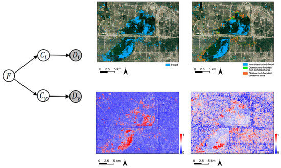
The structure of the Bayesian network for flood mapping based on the fusion of intensity and coherence is visualized in Figure 1a. It combines information from both the backscatter intensity and interferometric coherence time series. The shaded nodes in Figure 1 indicate observed variables whereas open nodes mask unknown variables. In detail, the random variable $\mathrm{F}$ indicates the flood state (e.g., $\mathrm{F}=1$ for flood state and $\mathrm{F}=0$ for non-flood state, respectively) of each pixel; this is our target variable for which we want to infer its posterior probability conditioned on all the other variables. The variable $\mathrm{D}$ corresponds to the combination of intensity and coherence time series: stacked imagery of multitemporal intensity and coherence. $\mathrm{C}$ is a hidden variable, which links the influence of variable $\mathrm{F}$ on the observed image series $\mathrm{D}$. It is difficult to find a simple causality between flood state and the observed SAR signatures, especially in urban areas associated with the complex backscattering mechanisms due to varying land covers. Therefore, it is necessary to introduce an intermediate variable $\mathrm{C}$ with K possible states that represent different temporal behaviors of the area of interest (AOI), corresponding to different land covers from a SAR (e.g., intensity and coherence) point of view [43,48]. Intensity and coherence characterize different physical properties of a scene: intensity provides information about surface roughness and permittivity, whereas coherence measures the random variation of individual scatterers between two SAR acquisitions, indicating temporal similarity within a cell. Therefore, intensity and coherence could be sensitive to and provide useful information on different flooded land covers. For instance, intensity is sensitive to flooded bare soils and flooded vegetation, both intensity and coherence are sensitive to flooded built-up areas, and coherence is also sensitive to some flooded built-up areas that are insensitive for intensity (as described in the Introduction section). Considering this phenomenon, the hidden variable $\mathrm{C}$ is decoupled to two variables of ${\mathrm{C}}_i$ and ${\mathrm{C}}_{\gamma }$ corresponding to the intensity and coherence temporal signature, respectively (Figure 1b), as the flood state of a given class $\mathrm{C}=k$, $k=1,\cdots ,\mathrm{K}$, should be evaluated from the perspective of intensity (e.g., $p\left(F|C_i=k\right)$) and coherence (e.g., $p\left(F|C_{\gamma }=k\right)$). The variable $\mathrm{D}$ is partitioned to intensity (e.g., variable ${\mathrm{D}}_i$) and coherence series (e.g., variable ${\mathrm{D}}_{\gamma }$) accordingly. The land cover segmentation (e.g., variable $\mathrm{C}$) is implemented under the conjunction of intensity and coherence time series (e.g., variable $\mathrm{D}$) to retain the internal dependencies between these two data sources and preserve compact clusters of the AOI. Another reason is that the conditional probabilities of $p\left(F|C_i\right)$ and $p\left(F|C_{\gamma }\right)$ are evaluated interactively (described in detail later in this section). Therefore, consistent clusters of intensity and coherence are required.

The joint probability of $p\left({\mathrm{D}}_i,{\mathrm{D}}_{\gamma }, F\right)$ in Figure 1b is given by:

$$p\left({\mathrm{D}}_i,{\mathrm{D}}_{\gamma }, F\right)= {{\displaystyle \sum }}_{C_i}p\left({\mathrm{D}}_i|C_i\right)p\left(C_i|F\right){{\displaystyle \sum }}_{C_{\gamma }}p\left({\mathrm{D}}_{\gamma }|C_{\gamma }\right)p\left(C_{\gamma }|F\right)p\left(F\right),$$

(2)

and the posterior probability of F = 1 can be expressed as:

$$p\left(F=1{|\mathrm{D}}_i,{\mathrm{D}}_{\gamma }\right)= \frac{{{\displaystyle \sum }}_{C_i}p\left({\mathrm{D}}_i|C_i\right)p\left(C_i|F=1\right){{\displaystyle \sum }}_{C_{\gamma }}p\left({\mathrm{D}}_{\gamma }|C_{\gamma }\right)p\left(C_{\gamma }|F=1\right)p\left(F=1\right)}{{{\displaystyle \sum }}_F{{\displaystyle \sum }}_{C_i}p\left({\mathrm{D}}_i|C_i\right)p\left(C_i|F\right){{\displaystyle \sum }}_{C_{\gamma }}p\left({\mathrm{D}}_{\gamma }|C_{\gamma }\right)p\left(C_{\gamma }|F\right)p\left(F\right)},$$

(3)

where $p\left(C_i|F\right)$ and p(C_γ|F) can be calculated via the Bayes rule:

$$p\left(C_j|F\right)= \frac{p\left(F|C_j\right)p\left(C_j\right)}{{{\displaystyle \sum }}_{C_j}p\left(F|C_j\right)p\left(C_j\right)},$$

(4)

with $j\in \left\{i, \gamma \right\}$.

Each term in Equation (3) can be calculated analytically. The distribution of $\mathrm{D}=\left(\begin{array}{c}{\mathrm{D}}_i\\ {\mathrm{D}}_{\gamma }\end{array}\right)$ is estimated by a finite Gaussian Mixture Model (GMM) involving the hidden variable $\mathrm{C}$. Each assignment of $\mathrm{C}$ is a Gaussian component, thus $p\left(D|C=k\right)=\mathcal{N}\left(D|{\mu }_k, {\mathsf{\Sigma }}_k\right)$, $k=1,\cdots ,\mathrm{K}$, and the parameters of each Gaussian component, $\left({\mu }_k, {\mathsf{\Sigma }}_k\right)$, ${\mu }_k=\left(\begin{array}{c}{\mu }_{ik}\\ {\mu }_{\gamma k}\end{array}\right)$, ${\mathsf{\Sigma }}_k=\left(\begin{array}{cc}{\mathsf{\Sigma }}_{iik}& {\mathsf{\Sigma }}_{i\gamma k}\\ {\mathsf{\Sigma }}_{\gamma ik}& {\mathsf{\Sigma }}_{\gamma \gamma k}\end{array}\right)$, are estimated by the expectation-maximization (EM) algorithm [49]. Therefore, $p\left({\mathrm{D}}_i|C_i=k\right)$ and $p\left({\mathrm{D}}_{\gamma }|C_{\gamma }=k\right)$ are also Gaussian densities and can be calculated by $p\left({\mathrm{D}}_i|C_i=k\right)=\mathcal{N}\left({\mathrm{D}}_i|{\mu }_{ik}, {\mathsf{\Sigma }}_{iik}\right)$ and $p\left({\mathrm{D}}_{\gamma }|C_{\gamma }=k\right)=\mathcal{N}\left({\mathrm{D}}_{\gamma }|{\mu }_{\gamma k},{\mathsf{\Sigma }}_{\gamma \gamma k}\right)$, respectively [46]. The number of Gaussian mixtures, K, depends on the homogeneity of the AOI. A smaller value of K is needed for a more homogeneous area. In practice, a relatively large K is preferable as under-clustering results in mixed clusters with variable spectral signatures and causes a compromised result, whereas over-clustering does not impact the final result [43]. We select K via the Bayesian information criterion (BIC). The flood prior probability $p\left(F=1\right)$ can be approximated by auxiliary data [43]. However, auxiliary data are not always available in emergency response and a SAR data self-consistent approach is more preferable. Therefore, the non-informative prior probability is used in this paper, $p\left(F=1\right)=p\left(F=0\right)=0.5$.

The term $p\left(C_j\right)$ in Equation (4) is a vector of weights of K Gaussian components. $p\left(F|C_j\right)$ is a conditional probability table (CPT) that contains the flood probability of each component. It is the core part of the whole process and determines the final result. The CPT can be assigned manually by an expert or be learned from the data. The latter strategy is adopted in this paper to make the whole chain automatic. Under the assumption that the existence of floodwater may cause an abrupt change in either intensity or coherence, the CPT is estimated based on the variation between the average of pre-event series and the co-event acquisition for each component centroid (e.g., ${\mu }_{jk}$, $j\in \left\{i, \gamma \right\}$, and $k=1,\cdots ,\mathrm{K}$). Intensity could decrease or increase due to the specular reflection or double-bounce, whereas coherence drops because of decorrelation caused by floodwater. Let ${\Delta }_j$, $j\in \left\{i, \gamma \right\}$ be the variation vector that we are concerned; we intend to extract the change information related to flooding at this step:

$$\begin{gathered} {\Delta }_i=max\left(mean\left({\mu }_i^{pre}\right), {\mu }_i^{co} \right)- min\left(mean\left({\mu }_i^{pre}\right), {\mu }_i^{co} \right), \\ {\Delta }_{\gamma }=mean\left({\mu }_{\gamma }^{pre}\right)-{\mu }_{\gamma }^{co}, \end{gathered}$$

(5)

where $max\left(·, ·\right)$ and $min\left(·, ·\right)$ extract the element-wise maximum and minimum values of two vectors, respectively, $mean(·)$ is the average operator along the time axis, ${\mu }_j^{pre}$ and ${\mu }_j^{co}$ represent component centroids of the pre-event series and the co-event acquisition, respectively. The CPT $p\left(F|C_j\right)$ is given by the sigmoid function of ${\Delta }_j$:

$$p\left(F|C_j\right)= \frac{1}{1+e^{-{\beta }_j\left({\Delta }_j-{\alpha }_j\right)}},$$

(6)

where ${\beta }_j$ is the steepness of the curve, and ${\alpha }_j$ is the ${\Delta }_j$ value corresponding to $p\left(F|C_j\right)=0.5$. With relatively steep curves, the final result is not sensitive to the value of ${\beta }_j$ and ${\beta }_j=1$ is set as the default value. ${\alpha }_j$ is the most important parameter and an optimal value should be assigned. After ${\Delta }_j$ is computed through Equation (5), its values are sorted in descending order. ${\Delta }_{jl}$ ($l=1,\cdots ,\mathrm{K}-1$) is the potential value of ${\alpha }_j$ and it separates the components to a flood-related changed set ${\Phi }_{jC}$ (${\Delta }_{jk}\in {\Phi }_{jC}, k\le l$) and an unchanged set Φ_jU (${\Delta }_{jk}\in {\Phi }_{jU}, k>l$). A cost function is defined to find the optimal index of $l^{*}$ by measuring intraclass compactness and interclass separability of the two sets [50,51]:

$$L_l= \frac{{{\displaystyle \sum }}_{V=\left\{C,U\right\}}{{\displaystyle \sum }}_{\forall {\Delta }_{jk}\in {\Phi }_{jV}}{\left({\Delta }_{jk}-m_{jV}\right)}^2}{{{\displaystyle \sum }}_{V=\left\{C,U\right\}}\frac{N_{{\Phi }_{jV}}}{K}{\left(m_{jV}-m_j\right)}^2},$$

(7)

where $m_{jV}$ is the mean value of set Φ_jV, $N_{{\Phi }_{jV}}$ is the component number of set ${\Phi }_{jV}$, and $m_j$ is the mean value of the whole ${\Delta }_j$. A smaller value of $L_l$ achieves higher intraclass compactness and interclass separability, thus $l^{*}$ is determined via the minima of Equation (7):

$$l^{*}= arg\underset{l}{\min }\left\{L_l\right\}, l=1,\cdots ,\mathrm{K}-1$$

(8)

The CPT $p\left(F|C_j\right)$ needs to be further refined after being calculated via Equations (5)–(8), since we should take into account the flood uncertainty in terms of intensity and coherence depends on the land cover types. Generally speaking, the change information from intensity is reliable for flood detection in non-built-up areas and partially reliable for built-up areas. Missed alarms that happen in some particular built-up areas (see the Introduction section) need the complement of coherence information. The change information from coherence is reliable for coherent targets (e.g., built-up areas) and not reliable for non-coherent areas such as vegetated areas - especially when data with large temporal baseline (e.g., from days up to months) are used. Moreover, the different temporal baselines between the pre-event acquisitions and the co-event acquisition can also cause either false alarms or missed alarms in non-coherent areas. Therefore, we first classify the AOI to coherent (built-up) and non-coherent (non-built-up) areas through the relationship between $mean\left({\mu }_{\gamma }^{pre}\right)$ and a threshold $t$, and subsequently refine $p\left(F|C_i\right)$ and $p\left(F|C_{\gamma }\right)$ as:

$$\begin{gathered} p\left(F|C_{ik}\in \left\{\left[mean\left({\mu }_{\gamma k}^{pre}\right)>t\right]\&\left[({\Delta }_{ik}<{\alpha }_i)\&({\Delta }_{\gamma k}>{\alpha }_{\gamma })\right]\right\}\right)=0.5, \\ p\left(F|C_{\gamma k}\in \left\{\left[mean\left({\mu }_{\gamma k}^{pre}\right)\le t\right]\&\left[\left[({\Delta }_{ik}>{\alpha }_i)\&({\Delta }_{\gamma k}<{\alpha }_{\gamma })\right]\left|\right|\left[({\Delta }_{\gamma k}>{\alpha }_{\gamma })\&({\Delta }_{ik}<{\alpha }_i)\right]\right]\right\}\right)=0.5, \end{gathered}$$

(9)

where $\&$ denotes the logical AND, and $\left|\right|$ denotes the logical OR, respectively. Equation (9) refines the flood evidence in terms of intensity and coherence according to the category of each component. For a given component $k$ which belongs to the coherent (built-up) areas, when the flood evidence is favored by coherence (e.g.,${\Delta }_{\gamma k}>{\alpha }_{\gamma }$) whereas not by intensity (e.g., ${\Delta }_{ik}<{\alpha }_i$), intensity may fail to capture the flood information. Therefore, $p\left(F|C_{ik}\right)=0.5$ is assigned to this component to account for the uncertainty of intensity. For components that belong to non-coherent (non-built-up) areas, on the one hand, the non-flooded one can be misclassified as a flooded component by coherence due to the large temporal variation of the land cover and the (possible) difference of temporal baseline in the dataset. On the other hand, when pre-event coherence of a flooded component is already low (e.g., vegetated areas), neglectable variation can be observed between pre- and co-event coherence, thus it is difficult to detect floodwater by coherence. Therefore, $p\left(F|C_{\gamma k}\right)=0.5$ is assigned to the non-coherent components which show inconsistent flood evidence from intensity and coherence.

After the final $p\left(F|C_j\right)$ is determined, the flood posterior probability of each pixel can be evaluated through Equations (3) and (4). The fully-connected CRF is adopted to refine the flood probability by integrating the long-range spatial information and the final binary flood extent is obtained via the maximum a posteriori (MAP) operation. In this process, the flood posterior probability of each pixel estimated via the Bayesian network is the unary potential term of the fully-connected CRF, and the difference images calculated by Equation (5) are the feature vectors of the appearance kernel [18]. Finally, the binary flood extent can be further classified to the following flood categories: non-obstructed-flood that is characterized by a decreased σ° in co-event acquisition; obstructed-flooded non-coherent areas (e.g., flooded vegetation and vegetated built-up areas) that show an increased σ° in the co-event acquisition and low pre-event γ; obstructed-flooded coherent areas (e.g., flooded predominantly built-up areas) that present an increased/unchanged σ° in co-event acquisition and high pre-event γ.

3. Data and Experiments

Two case studies were conducted with different SAR sensors to test our method. The first case is the Houston (US) flood accompanying Hurricane Harvey which took landfall on 25 August 2017 on Texas. Harvey moved on to Houston on August 26 and remained there for four days. The local National Weather Service office in Houston observed daily rainfall accumulations of 370 mm and 408 mm on August 26 and 27, respectively [36]. Multiple flash flood emergency alerts were issued in the Houston area by the night of August 26. The study area is located at the western part of Houston city with an extension of ca. 590 km², which is mainly occupied by residential houses/apartments, commercial and industrial districts, parks, and reservoirs. Eleven Sentinel-1 (C band, 20 m resolution, five Sentinel-1A and six Sentinel-1B) VV polarized Interferometric Wide Swath (IW) mode Single Look Complex (SLC) data acquired between 1 July 2017 and 30 August 2017 (with 6 days repetition rate) were used. Intensity and coherence data details are shown in

Table 1. Sentinel-1 intensity data used for the Houston case study (flood acquisition is marked in blue color).

Acquisition Time	Polarization	Incidence Angle (°)	Resolution (m)	Orbit
01/07/17	VV	36.7	20	Descending
07/07/17	VV	36.7	20	Descending
13/07/17	VV	36.7	20	Descending
19/07/17	VV	36.7	20	Descending
25/07/17	VV	36.7	20	Descending
31/07/17	VV	36.7	20	Descending
06/08/17	VV	36.7	20	Descending
12/08/17	VV	36.7	20	Descending
18/08/17	VV	36.7	20	Descending
24/08/17	VV	36.7	20	Descending
30/08/17	VV	36.7	20	Descending

and

Table 2. Sentinel-1 coherence data used for the Houston case study (flood acquisition is marked in blue color).

Acquisition Time	${\mathit{B}}_{\mathit{t}}\left(\mathbf{days}\right)$	${\mathit{B}}_{\mathit{p}}\left(\mathbf{m}\right)$	Window Size (Range $\times$ Azimuth)
01/07 – 07/07	6	47	28 $\times$ 7
07/07 – 13/07	6	31	28 $\times$ 7
13/07 – 19/07	6	79	28 $\times$ 7
19/07 – 25/07	6	45	28 $\times$ 7
25/07 – 31/07	6	38	28 $\times$ 7
31/07 – 06/08	6	38	28 $\times$ 7
06/08 – 12/08	6	52	28 $\times$ 7
12/08 – 18/08	6	58	28 $\times$ 7
18/08 – 24/08	6	82	28 $\times$ 7
24/08 – 30/08	6	55	28 $\times$ 7

, respectively, with the flood acquisition marked in blue color. Intensity images were preprocessed by radiometric calibration, speckle reduction with the Refined Lee speckle filter (window size of 7 $\times$ 7 pixels), and converted from linear to dB. Coherence images were obtained by sequential image pairs with a 28 $\times$ 7 (Range $\times$ Azimuth) window. Multi-looking with a 4 $\times$ 1 window was performed to all images to get a square pixel. All intensity and coherence images were stacked and geocoded with the 30 m Shuttle Radar Topography Mission (SRTM) digital elevation model (DEM) to WGS1984 UTM Zone 15 N with a square pixel size of 15 m. Each image was scaled to the range (0,255) before the subsequent processing. The coherent (built-up) area filter was set as $t=0.5$ (0.5 * 255 for the scaled coherence images) suggested by Watanabe et al. [52] and Lu et al. [53]. The number of Gaussian components in this case study was $k=100$. The validation dataset was virtually digitized based on aerial photographs with a spatial resolution of 35 cm acquired on 30–31 August 2017 by the National Oceanic and Atmospheric Administration (NOAA) Remote Sensing Division [54].

The second case study is the Joso (Japan) flood caused by the Kanto-Tohoku heavy rainfall on 9–11 September 2015 and the collapsed bank of Kinugawa River. The maximum rainfall accumulations exceeded 600 mm in the Kanto region and 500 mm in the Tohoku region, respectively. The water volume of the Kinugawa River increased rapidly in the city of Joso in the early morning of 10 September, and the floodwater quickly covered almost the entire area between Kinugawa River and Kokai River (Figure 5) at 12:50 pm local time [55]. The inundation area decreased from ca. 31 km² on 11 September to ca. 2 km² on 16 September [56]. The study area consists of the Joso city area and a wide rice paddy field located to the north of Joso city with an extension of ca. 114 km². Seven ALOS-2/PALSAR-2 (L band, 3 m resolution) HH polarized Stripmap mode (SM1) SLC data were obtained for this study case. Intensity and coherence data details are shown in

Table 3. ALOS-2/PALSAR-2 intensity data used for the Joso case study (flood acquisition is marked in blue color).

Acquisition Time	Polarization	Incidence Angle (°)	Resolution (m)	Orbit
29/08/14	HH	35.4	3	Ascending
02/01/15	HH	35.4	3	Ascending
13/02/15	HH	35.4	3	Ascending
31/07/15	HH	35.4	3	Ascending
11/09/15	HH	35.4	3	Ascending
23/10/15	HH	35.4	3	Ascending
29/01/16	HH	35.4	3	Ascending

and

Table 4. ALOS-2/PALSAR-2 coherence data used for the Joso case study (flood acquisition is marked in blue color).

Acquisition Time	${\mathit{B}}_{\mathit{t}}\left(\mathbf{days}\right)$	${\mathit{B}}_{\mathit{p}}\left(\mathbf{m}\right)$	Window Size (Range $\times$ Azimuth)
29/08 – 02/01	126	150	7 $\times$ 7
02/01 – 13/02	42	47	7 $\times$ 7
13/02 – 31/07	168	221	7 $\times$ 7
31/07 – 11/09	42	123	7 × 7
11/09 – 23/10	42	35	7 $\times$ 7
23/10 – 29/01	98	205	7 $\times$ 7

, respectively, with the flood acquisition marked in blue color. The same preprocessing procedures as in the above case were performed concerning intensity and coherence except that the multi-looking step was omitted and coherence images were obtained with a 7 $\times$ 7 (Range $\times$ Azimuth) window. All images were geocoded with the 30 m SRTM DEM to WGS1984 UTM Zone 54N with a square pixel size of 2.5 m. The same experimental configuration of the Houston case was set: each data was scaled to the range (0,255) and $t=0.5$ was assigned. The number of Gaussian components in this case study was $k=40$. It is worth noting that the acquired data span across several seasons. To mitigate the impacts from the phenological variation of rice paddy, the intensity mean values of the pre-event acquisitions were only calculated by the acquisitions that dated in the same season of the co-event data. Therefore, only intensity data acquired on 29 August 2014 and 31 July 2015 were used for the average operation. Both 31 July 2015–11 September 2015 and 11 September 2015–23 October 2015 coherence pairs were co-event acquisitions and only the former was used. Besides, to mitigate the perturbation of $B_p$, coherence of 2 January 2015–13 February 2015 was not used in the experiment. The validation dataset was virtually digitized on the basis of aerial photographs with a spatial resolution of 20 cm acquired on 11 September 2015 by the Geospatial Information Authority of Japan (GSI) [57].

4. Results and Discussion

The results of two case studies are both qualitatively and quantitatively analyzed. The synoptic view of multi-temporal SAR data in the form of RGB combinations is widely used in the qualitative interpretation of land cover and surface dynamics [58,59]. Different RGB combinations are adopted to give an intuition of flood extent in terms of intensity and coherence. For both cases, the results obtained from the fusion of intensity and coherence, and from intensity alone are quantitively analyzed. The overall accuracy (OA), kappa coefficient (κ), false-positive rate (FPR), precision (i.e., the correctly predicted positive patterns from the total predicted patterns in a positive class), recall (i.e., the fraction of positive patterns that are correctly classified), and F1 score (i.e., the harmonic mean between recall and precision) [60] are reported based on the flood reference derived from the aerial photographs mentioned in Section 3. In addition, the temporal variation of intensity and coherence as a result of flooding over different land cover types are also analyzed and discussed.

4.1. Houston Flood Case

Figure 2a shows the intensity RGB composite (R = pre-event, G = B = co-event) of the Houston study area. The red color indicates non-obstructed-flood, such as flooded bare soils or wholly submersed short vegetations, without double-bounce occurring between the water surface and buildings/tree trunks. The cyan color depicts the flooded buildings or partially submersed vegetation where the enhanced double-bounce between the water surface and buildings/tree trunks incurs an increase in the co-event σ°. The coherence RGB composite (R = pre-event, G = B = co-event) is shown in Figure 2b. The white color shows non-flooded built-up areas which are characterized by high γ in both pre-event and co-event acquisitions. The appearance of floodwater between buildings results in a significant drop-off in co-event γ which are illustrated in the red color. However, the drop-off in γ could also be owing to random variation of vegetation (note the widely spread red color), thus the temporal non-coherent targets should be masked out when using γ in flood detection, as we discussed in Section 2. In Figure 2c, the RGB composite of intensity and coherence is adopted (R = co-event σ°, G = pre-event γ, and B = co-event γ). The flooded built-up areas are discernible in yellow color (e.g., high co-event σ°, high pre-event γ, and low co-event γ). The green color could be related to flooded bare soils with sparse meadow which are characterized by low co-event σ°, medium pre-event γ, and low co-event γ. Non-flooded built-up areas are shown in white color. Besides, the study area is quite vegetated, some small houses are encircled by trees, the mixed backscattering of the aforementioned objects could be presented in a single pixel of the medium resolution (e.g., 20 m) Sentinel-1 data, thus attenuating the double-bounce effect of buildings and reducing the values of both σ° and γ. These areas can be found in brown color in Figure 2c.

The quantitative evaluations of the flood extent in the study area (Figure 2) produced by the fusion of σ° and γ (Figure 3a) and σ° alone (Figure 3c) are reported in

Table 5. Quantitative evaluation of the Houston flood case (FPR: false-positive rate, OA: overall accuracy).

	Data	Precision	Recall	F1	FPR	OA (%)	κ
Houston city	Intensity + Coherence	0.83	0.61	0.70	0.02	94.5	0.68
	Intensity	0.85	0.50	0.63	0.01	93.7	0.60

. Although high values of OA (e.g., 94.5% vs. 93.7%) are achieved for both scenarios, OA is an inappropriate evaluation metric for this case due to the unbalanced extent of the classes (e.g., flood class occupies around 10% of the whole area). When σ° and γ are synergistically used, κ is around 0.68 and F1 score is around 0.70. Comparing the extracted flood extent in Figure 3a with the reference flood mask in Figure 3d it can be found that the spatial pattern of flooded areas is extracted accurately. The overestimation is very low (e.g., 0.02), however, a relatively large underestimation can be found, with 0.61 recall. The underestimated inundation areas are mainly flooded dense built-up areas with heavy vegetation. In these areas, pre-event coherence is expected to be low and the canopy attenuates the double-bounce scattering occurring between floodwater surfaces and building walls. Thus, it is difficult to detect either a significant increase in σ° or decrease in γ between the pre- and co-event acquisitions. Figure 3b provides an insight of distributions of different flood categories: non-obstructed-flood; obstructed-flooded non-coherent areas such as vegetation and vegetated built-up areas; and obstructed-flooded coherent areas, predominantly built-up areas. When only σ° data are used, lower κ (e.g., 0.60) and F1 score (e.g., 0.63) are achieved with slight differences in precision and FPR compared to the joint use of σ° and γ. Figure 3c shows a larger underestimation especially in built-up areas compared to Figure 3a,b, corresponding to a lower recall value of 0.50. To gain an insight of the contributions from σ° and γ in urban flood detection, Figure 3e,f show the flood posterior probability conditioned on σ° and γ, respectively, providing a perception of distribution of the flood evidence that supported by σ° and γ. It can be found that the detected non-obstructed-flood in Figure 3b is dominantly determined by σ°. Flooded built-up areas are captured by both σ° and γ but γ adds further comprehensive flood information.

To get a better understanding of the roles of σ° and γ for flood detection in urban environments, we explore the temporal variation of spatial average values of σ° and γ in 4 regions that represent different flooded land-cover types, as shown in Figure 4. R#1 is a homogenous short vegetation area that is (almost) wholly submerged in the flood event, the pre-event γ is low in this area (e.g., the maximum value is 0.27 and mean value is 0.18). Although the appearance of floodwater leads to a lower co-event γ (e.g., 0.12), γ is not reliable information for flood detection in this area because of the low values and large variation of the pre-event γ. The pre-event σ° is around −8.5 dB characterized by mixed surface and volume backscattering, however, the co-event σ° decreases significantly to −13.7 dB due to the specular reflection results from floodwater surface. Thus, σ° provides useful information for flood detection in this area. R#2 is a predominantly built-up area. High pre-event γ (e.g., around 0.85) holds for this temporally stable area, the appearance of floodwater results in a significant drop-off in the co-event γ (e.g., 0.35). Besides, the co-event σ° also increases substantially by the enhanced double-bounce effect, from around −5.5 dB to −0.3 dB. Therefore, both σ° and γ are useful for flood detection in this area. R#3 consists of building blocks with trees. The pre-event γ of this area is around 0.36, which could be attributed to the existence of trees and anthropogenic activities in the streets around buildings. The co-event γ drops to 0.14, nevertheless, this drop-off is much less significant than that in R#2 and as this area is weakly coherent, γ is not helpful for flood detection in this area. The pre-event σ°, however, increases from around −9.0 dB to −4.8 dB in co-event σ°. The wide spaces between buildings and the relatively small ϕ between building orientation and the SAR azimuth direction probably facilitate the enhancement of the double-bounce effect in the co-event acquisition. Thus, σ° is more informative than γ for flood detection in this area. R#4 is an underestimated inundation area of dense buildings surrounded by trees. In this area, the pre-event γ drops from around 0.60 to 0.32 in the co-event γ, whereas the pre-event σ° increases from around −7.0 dB to −6.0 dB in co-event σ°. The variations in both σ° and γ are less considerable than the successfully detected flooded built-up areas, e.g., a 0.28 drop-off of γ compared to a 0.5 drop-off in R#2, a 1 dB increase of σ° compared to a 5.2 dB increase in R#2 and a 4.2 dB increase in R#3. Since the buildings, trees and streets are densely distributed, γ is estimated with the mixed structures especially in medium resolution data such as Sentinel-1, thus attenuating the drop-off in the co-event γ. On the other hand, the double-bounce backscattering between floodwater surface and buildings could be obstructed by trees, and the floodwater could also be masked by shadow. Therefore, flood detection in this scenario is challenging especially for medium resolution data (e.g., 10 to 30 m).

4.2. Joso Flood Case

The intensity RGB composite (R = pre-event, G = B = co-event) of the Joso study area is shown in Figure 5a. The red color indicates flooded rice paddy, whereas cyan color hints potential flooded built-up areas and partially submersed vegetation, also including broadly spread vegetation that presents higher co-event σ° than the pre-event one probably due to potential phenological variation. The white color displays built-up areas and some paddy fields on which occur strong double-bounce effects in both acquisitions. Figure 5b visualizes the coherence RGB composite (R = pre-event, G = B = co-event). The red color illustrates flooded built-up areas, some rural roads, and fields which are characterized by a high value of γ in L band pre-event data. The colorful appearance of RGB composite of intensity and coherence (R = co-event σ°, G = pre-event γ, and B = co-event γ) in Figure 5c holds a wealth of information on the flood situation in different land-cover classes. The white color shows non-flooded built-up areas whereas flooded built-up areas are shown in yellow color. The green color illustrates the flooded coherent rural roads and fields that have low co-event σ°, high co-event σ°, and low co-event γ. The black color reveals flooded rice paddy fields and permanent water such as the course of the rivers through the northern and southern part of the study area. Vegetation is depicted in red color which is largely distributed along the rivers. The purple color locates some non-flooded paddy fields that have high co-event γ and low pre-event γ probably due to the larger temporal baseline of pre-event γ (e.g., 168 days across seasons) compared to the co-event γ (e.g., 42 days in the same season).

As the study area contains both urban and rural areas and we intend to mainly focus on flood detection in urban areas in this paper. We report the quantitative evaluations for both the whole study area (Figure 5) and the urban area of Joso city which is located in the yellow dashed rectangle in Figure 6a.

Table 6. Quantitative evaluation of the Joso flood case (FPR: false-positive rate, OA: overall accuracy).

	Data	Precision	Recall	F1	FPR	OA (%)	κ
Whole study area	Intensity + Coherence	0.91	0.70	0.79	0.03	89.6	0.72
	Intensity	0.85	0.59	0.70	0.04	86.0	0.61
Joso city	Intensity + Coherence	0.94	0.66	0.78	0.03	84.3	0.66
	Intensity	0.85	0.45	0.59	0.06	74.0	0.42

lists the evaluations of results produced by the fusion of σ° and γ (Figure 6a,g) and σ° alone (Figure 6c,i). When combining σ° and γ, the result for the urban area is slightly worse than for the whole area in terms of OA (e.g., 84.3% vs. 89.6%) and κ (e.g., 0.66 vs. 0.72). This degradation is mainly due to a larger underestimation in urban areas, e.g., 0.66 of recall compared to 0.70 in the whole area. This difference is enlarged when only σ° data are used (e.g., 74.0% vs. 86.0% for OA and 0.42 vs. 0.61 for κ). The occurrence of specular surfaces, such as parking lots and shadowing caused by buildings/trees, can degrade the performance in urban areas. According to the mapping result shown in Figure 6a,b, the underestimation primarily appears in parking lots, densely distributed built-up areas and bare fields that show a similar σ° in dry and flooded situations in the rural area. A subtle overestimation is found in both validation areas (e.g., 0.03 in both areas). Figure 6b,h show the distribution of different flood categories and indicate that the obstructed-flooded non-coherent areas are largely distributed accompanying the obstructed-flooded coherent areas. This is rational as the presence of vegetation and anthropogenic activities reduce the coherence of built-up areas. The overall performance degrades when σ° is used by itself. A large area falsely detected as flooded can be seen in Figure 6c (close to the right bottom corner of the yellow rectangle) due to the variation of σ° in rice paddy field, and a severe underestimation can be found in the Joso city area (Figure 6i) with a low recall value of 0.45. Figure 6e,f illustrate flood posterior probability conditioned on σ° and γ, respectively. It can be found that σ° provides very strong evidence in flooded rice paddy areas but a weaker one in flooded built-up areas. However, γ complements the flood information of built-up areas and other coherent areas such as rural roads.

Figure 7 shows the temporal variation of the spatial average values of σ° and γ over 6 different regions. R#1 is a completely flooded homogeneous rice paddy field. Flooding causes a significant decrease of σ° in this area, ranging from around −2.5 dB of pre-event σ° (only considering acquisitions on 29 August 2014 and 31 July 2015) to −16 dB of co-event σ°, whereas the change of γ (e.g., 0.03) between pre- and co-event data is hardly detectable. R#2 and R#3 are flooded built-up areas observed with different ϕ angles. R#2 has a smaller ϕ than R#3. It can be found that the increase of co-event σ° caused by double-bounce in R#2 is larger than R#3 (e.g., around 3.6 dB against 1.6 dB). However, the drop-off in co-event γ has less difference between R#2 and R#3 (e.g., 0.30 against 0.31). It indicates that γ as a complement to σ° can help identify floodwater in built-up areas where might fail to detect by σ° alone. Besides, the effect of ϕ can be mitigated by combing the descending and ascending acquisitions that observe the same area from different viewing angles and increase the chance of floodwater detection. R#4 consists of flooded trees. It shows a strong double-bounce effect between floodwater and tree trunks thanks to the high penetration capability of L-band. The backscattering σ° increases from around −8.0 dB to −5.3 dB when inundation appears. Without surprise, the variation between pre- and co-event γ (e.g., 0.04) is as subtle as for R#1. The regions of R#5 and R#6 are corresponding to underestimated flooded parking lots and dense building blocks, respectively. For R#5, γ changes from around 0.31 in pre-event to 0.23 in co-event data. Due to busy anthropogenic activities, the low pre-event γ attenuates the γ variation caused by flooding over time and thus hampers flood detection based on γ. On the other hand, both pre- and co-event σ° are very low (e.g., −14.8 dB against −14.6 dB), as the backscattering from parking lots in dry conditions is also specular. Therefore, flood detection in parking lots could be challenging for both σ° and γ. In the dense built-up area of R#6, radar shadows hamper flood detection in the front of buildings and the evidence of flood from σ° is unnoticed. As the scatters are probably dominated by the roofs, the co-event γ is as high as the pre-event γ (e.g., above 0.6). Apart from the reasons of underestimation we discussed for R#5 and R#6, the underestimation in Joso city is also probably due to a floodwater recession at the time of SAR acquisition, since the inundation extent varies rapidly in time according to the inundation maps provided by GSI [56] and a large inundation area in Joso city disappeared on 12 September 2015. A large white area between the red areas in Joso city can be found in Figure 5b, which indicates that there is no significant coherence decorrelation occurring in this area.

4.3. Limitations and Future Directions

The main limitations of the proposed method lie in data availability and scalability. Although the method is flexible to data availability that both (long) time series or bi-temporal data can be used, a longer time series produces more unbiased coherent-area estimation and subsequently achieves a better CPT. For satellite missions with irregular observation scenarios such as ALOS-2/PALSAR-2 and TerraSAR-X, it can be hard to achieve a long time series of images with consistent acquisition parameters. Nevertheless, this does not mean that the method will fail to succeed with fewer multi-temporal data, as shown in the Joso case of this study. Promising results are achieved with less than 5 coherence sequence. This could benefit from the high spatial resolution of ALOS-2/PALSAR-2 data (e.g., 3 m) so that the coherence of built-up areas can be estimated with more pure pixels thus showing low temporal variation. For data with a lower spatial resolution such as Sentinel-1 data (e.g., 20 m), a longer data sequence is preferable. Data acquisition is going to be a less crucial problem with the evolution of SAR missions. Satellite constellations such as the Sentinel-1 mission and the recently launched RADARSAT Constellation Mission (RCM) [61] with high temporal resolution can provide a long and dense observation sequence of an area of interest, and the upcoming missions such Tandem-L [62] and NASA-ISRO SAR (NISAR) [63] will increase the observation frequency of spaceborne SAR systems at the global scale. The computation bottleneck of the method is the GMM with the EM algorithm. The best-case run time for the EM algorithm is ${\rm O}\left(KNd\right)$ at each iteration, where is the cluster number, $N$ is the data point number and $d$ is the data dimension. Therefore, it is challenging to scale for a massive dataset with high-dimension. One possible way to deal with the scalability problem is to leverage the advanced data summarization techniques such as the coreset-based GMM [64,65], which guarantees that models fitting the $M\left(M\ll N\right)$ coresets (weighted subsets of the original data) will also provide a good fit for the original dataset. Besides, the quality of SAR image segmentation also affects the calculation of CPT. Compared to the standard GMM used for segmentation in this paper, the spatial constraint GMM [66] which imposes the contextual information in the mixing coefficient can achieve a better segmentation quality.

5. Conclusions

In this paper, we introduced a method for flood mapping in urban environments based on SAR intensity and interferometric coherence under the Bayesian network fusion framework. It integrates intensity and coherence information from a viewpoint of probability and takes into account the flood uncertainty in terms of intensity and coherence. The combination of intensity and coherence extracts flood information in varying land cover types and outputs both flood binary extent and flood category maps: including non-obstructed-flood (e.g., flooded bare soils and short vegetation); obstructed-flooded non-coherent area (e.g., flooded vegetation and vegetated built-up areas); and obstructed-flooded coherent area (e.g., flooded predominantly built-up areas). The approach is unsupervised and only based on SAR data, therefore favorable for operational emergency response with data from SAR missions with a short revisit time and systematic observation scenario such as Sentinel-1.

This method was tested on two flood events that were captured by different SAR sensors: the Houston (US) 2017 flood event with Sentinel-1 (C band, 20 m resolution) time series, and the Joso (Japan) 2015 flood event with ALOS-2/PALSAR-2 (L band, 3 m resolution) time series. The flood maps were validated by the reference flood masks derived from high-resolution aerial photographs and showed satisfying results in both case studies. The findings in the experiments demonstrate that the synergistic use of SAR intensity and coherence provides more reliable flood information in urban areas with varying landscapes than using intensity alone. Specifically, flood detection in less-coherent/non-coherent areas (e.g., bare soils, vegetation, vegetated built-up areas) relies on multi-temporal intensity, whereas multi-temporal coherence gives more comprehensive flood information in coherent areas (e.g., predominantly built-up areas). Nevertheless, some special flood situations such as flooded parking lots and flooded dense building blocks are still challenging for both intensity and coherence.

As the proposed method is sensor and scene independent, it provides opportunities for urban flood mapping at a global scale and especially in low-income countries with the highly frequent and systematic observations from SAR missions such as Sentinel-1 and the RADARSAT Constellation Mission (RCM). The upcoming missions such as Tandem-L and NISAR increase the observation frequency of spaceborne SAR systems and the possibility of flood detection in vegetated areas. Besides, the proposed method provides a supplement to the current Sentinel-1 Flood Service at the German Aerospace Center (DLR) to account for flooding in urban areas.

References

- IDMC. Global Report on Internal Displacement. 2016. Available online: http://www.internal-displacement.org/globalreport2016/pdf/2016-global-report-internal-displacement-IDMC.pdf (accessed on 16 September 2019).
- Willner, S.N.; Levermann, A.; Zhao, F.; Frieler, K. Adaptation required to preserve future high-end river flood risk at present levels. Sci. Adv. 2018, 4, eaao1914. [Google Scholar] [CrossRef] [PubMed] [Green Version]
- Willner, S.N.; Otto, C.; Levermann, A. Global economic response to river floods. Nat. Clim. Chang. 2018, 8, 594–598. [Google Scholar]
- Covello, F.; Battazza, F.; Coletta, A.; Lopinto, E.; Fiorentino, C.; Pietranera, L.; Valentini, G.; Zoffoli, S. COSMO-SkyMed an existing opportunity for observing the Earth. J. Geodyn. 2010, 49, 171–180. [Google Scholar] [Green Version]
- Werninghaus, R.; Buckreuss, S. The TerraSAR-X Mission and System Design. IEEE Trans. Geosci. Remote Sens. 2009, 48, 606–641. [Google Scholar] [CrossRef]
- Torres, R.; Snoeij, P.; Geudtner, D.; Bibby, D.; Davidson, M.; Attema, E.; Potin, P.; Rommen, B.Ö.; Floury, N.; Brown, M.; et al. GMES Sentinel-1 mission. Remote Sens. Environ. 2012, 120, 9–24. [Google Scholar] [CrossRef]
- Morena, L.C.; James, K.V.; Beck, J. An introduction to the RADARSAT-2 mission. Can. J. Remote Sens. 2004, 30, 221–234. [Google Scholar] [CrossRef]
- Kankaku, Y.; Suzuki, S.; Osawa, Y. ALOS-2 mission and development status. In Proceedings of the 2013 IEEE International Geoscience and Remote Sensing Symposium—IGARSS, Melbourne, Australia, 21–26 July 2013; pp. 2396–2399. [Google Scholar]
- Matgen, P.; Hostache, R.; Schumann, G.; Pfister, L.; Hoffmann, L.; Savenije, H.H.G. Towards an automated SAR-based flood monitoring system: Lessons learned from two case studies. Phys. Chem. Earth Parts A/B/C 2011, 36, 241–252. [Google Scholar] [CrossRef]
- Martinis, S.; Twele, A.; Voigt, S. Towards operational near real-time flood detection using a split-based automatic thresholding procedure on high resolution TerraSAR-X data. Nat. Hazards Earth Syst. Sci. 2009, 9, 303–314. [Google Scholar]
- Shen, X.; Wang, D.; Mao, K.; Anagnostou, E.; Hong, Y. Inundation Extent Mapping by Synthetic Aperture Radar: A Review. Remote Sens. 2019, 11, 879. [Google Scholar] [CrossRef]
- Pulvirenti, L.; Chini, M.; Pierdicca, N.; Guerriero, L.; Ferrazzoli, P. Flood monitoring using multi-temporal COSMO-SkyMed data: Image segmentation and signature interpretation. Remote Sens. Environ. 2011, 115, 990–1002. [Google Scholar]
- Martinis, S.; Twele, A.; Voigt, S. Unsupervised Extraction of Flood-Induced Backscatter Changes in SAR Data Using Markov Image Modeling on Irregular Graphs. IEEE Trans. Geosci. Remote Sens. 2011, 49, 251–263. [Google Scholar] [CrossRef]
- Insom, P.; Cao, C.; Boonsrimuang, P.; Liu, D.; Saokarn, A.; Yomwan, P.; Xu, Y. A Support Vector Machine-Based Particle Filter Method for Improved Flooding Classification. IEEE Geosci. Remote Sens. Lett. 2015, 12, 1943–1947. [Google Scholar] [CrossRef]
- Twele, A.; Cao, W.; Plank, S.; Martinis, S. Sentinel-1-based flood mapping: A fully automated processing chain. Int. J. Remote Sens. 2016, 37, 2990–3004. [Google Scholar] [CrossRef]
- Chini, M.; Hostache, R.; Giustarini, L.; Matgen, P. A Hierarchical Split-Based Approach for Parametric Thresholding of SAR Images: Flood Inundation as a Test Case. IEEE Trans. Geosci. Remote Sens. 2017, 55, 6975–6988. [Google Scholar]
- Cao, W.; Twele, A.; Plank, S.; Martinis, S. A three-class change detection methodology for SAR-data based on hypothesis testing and Markov Random field modelling. Int. J. Remote Sens. 2018, 39, 488–504. [Google Scholar]
- Li, Y.; Martinis, S.; Plank, S.; Ludwig, R. An automatic change detection approach for rapid flood mapping in Sentinel-1 SAR data. Int. J. Appl. Earth Obs. Geoinf. 2018, 73, 123–135. [Google Scholar] [CrossRef]
- Tong, X.; Luo, X.; Liu, S.; Xie, H.; Chao, W.; Liu, S.; Liu, S.; Makhinov, A.N.; Makhinova, A.F.; Jiang, Y. An approach for flood monitoring by the combined use of Landsat 8 optical imagery and COSMO-SkyMed radar imagery. ISPRS J. Photogramm. Remote Sens. 2018, 136, 144–153. [Google Scholar]
- Schumann, G.J.; Moller, D.K. Microwave remote sensing of flood inundation. Phys. Chem. Earth 2015, 83–84, 84–95. [Google Scholar] [CrossRef]
- Dong, Y.; Forster, B.; Ticehurst, C. Radar backscatter analysis for urban environments. Int. J. Remote Sens. 1997, 18, 1351–1364. [Google Scholar]
- Franceschetti, G.; Iodice, A.; Riccio, D. A canonical problem in electromagnetic backscattering from buildings. IEEE Trans. Geosci. Remote Sens. 2002, 40, 1787–1801. [Google Scholar] [CrossRef]
- Thiele, A.; Cadario, E.; Karsten, S.; Thönnessen, U.; Soergel, U. Building Recognition From Multi-Aspect High-Resolution InSAR Data in Urban Areas. IEEE Trans. Geosci. Remote Sens. 2007, 45, 3583–3593. [Google Scholar] [CrossRef]
- Wegner, J.D.; Hansch, R.; Thiele, A.; Soergel, U. Building Detection From One Orthophoto and High-Resolution InSAR Data Using Conditional Random Fields. IEEE J. Sel. Top. Appl. Earth Obs. Remote Sens. 2011, 4, 83–91. [Google Scholar] [CrossRef]
- Ferro, A.; Brunner, D.; Bruzzone, L.; Lemoine, G. On the relationship between double bounce and the orientation of buildings in VHR SAR images. IEEE Geosci. Remote Sens. Lett. 2011, 8, 612–616. [Google Scholar]
- Mason, D.C.; Speck, R.; Devereux, B.; Schumann, G.J.-P.; Neal, J.C.; Bates, P.D. Flood Detection in Urban Areas Using TerraSAR-X. IEEE Trans. Geosci. Remote Sens. 2010, 48, 882–894. [Google Scholar]
- Mason, D.C.; Davenport, I.J.; Neal, J.C.; Schumann, G.J.-P.; Bates, P.D. Near Real-Time Flood Detection in Urban and Rural Areas Using High-Resolution Synthetic Aperture Radar Images. IEEE Trans. Geosci. Remote Sens. 2012, 50, 3041–3052. [Google Scholar] [CrossRef] [Green Version]
- Giustarini, L.; Hostache, R.; Matgen, P.; Schumann, G.J.; Bates, P.D.; Mason, D.C. A Change Detection Approach to Flood Mapping in Urban Areas Using TerraSAR-X. IEEE Trans. Geosci. Remote Sens. 2013, 51, 2417–2430. [Google Scholar] [CrossRef]
- Mason, D.C.; Giustarini, L.; Garcia-Pintado, J.; Cloke, H.L. Detection of flooded urban areas in high resolution Synthetic Aperture Radar images using double scattering. Int. J. Appl. Earth Obs. Geoinf. 2014, 28, 150–159. [Google Scholar] [Green Version]
- Tanguy, M.; Chokmani, K.; Bernier, M.; Poulin, J.; Raymond, S. River flood mapping in urban areas combining Radarsat-2 data and flood return period data. Remote Sens. Environ. 2017, 198, 442–459. [Google Scholar] [CrossRef] [Green Version]
- Pulvirenti, L.; Chini, M.; Pierdicca, N.; Boni, G. Use of SAR data for detecting floodwater in urban and agricultural areas: The role of the interferometric coherence. IEEE Trans. Geosci. Remote Sens. 2016, 54, 1532–1544. [Google Scholar]
- Iervolino, P.; Guida, R.; Iodice, A.; Riccio, D. Flooding water depth estimation with high-resolution SAR. IEEE Trans. Geosci. Remote Sens. 2015, 53, 2295–2307. [Google Scholar]
- Chini, M.; Pulvirenti, L.; Pierdicca, N. Analysis and interpretation of the COSMO-SkyMed observations of the 2011 Japan tsunami. IEEE Geosci. Remote Sens. Lett. 2012, 9, 467–471. [Google Scholar] [CrossRef]
- Zebker, H.A.; Member, S.; Villasenor, J. Decorrelation in Interferometric Radar Echoes. IEEE Trans. Geosci. Remote Sens. 1992, 30, 950–959. [Google Scholar] [CrossRef]
- Li, Y.; Martinis, S.; Wieland, M. Urban flood mapping with an active self-learning convolutional neural network based on TerraSAR-X intensity and interferometric coherence. ISPRS J. Photogramm. Remote Sens. 2019, 152, 178–191. [Google Scholar] [CrossRef]
- Chini, M.; Pelich, R.; Pulvirenti, L.; Pierdicca, N.; Hostache, R.; Matgen, P. Sentinel-1 InSAR Coherence to Detect Floodwater in Urban Areas: Houston and Hurricane Harvey as A Test Case. Remote Sens. 2019, 11, 107. [Google Scholar] [CrossRef]
- Marcot, B.G.; Penman, T.D. Advances in Bayesian network modelling: Integration of modelling technologies. Environ. Model. Softw. 2019, 111, 386–393. [Google Scholar]
- Cheon, S.P.; Kim, S.; Lee, S.Y.; Lee, C.B. Bayesian networks based rare event prediction with sensor data. Knowl. Based Syst. 2009, 22, 336–343. [Google Scholar]
- Landuyt, D.; Broekx, S.; D’hondt, R.; Engelen, G.; Aertsens, J.; Goethals, P.L.M. A review of Bayesian belief networks in ecosystem service modelling. Environ. Model. Softw. 2013, 46, 1–11. [Google Scholar] [CrossRef]
- Chen, J.; Ping-An, Z.; An, R.; Zhu, F.; Xu, B. Risk analysis for real-time flood control operation of a multi-reservoir system using a dynamic Bayesian network. Environ. Model. Softw. 2019, 111, 409–420. [Google Scholar] [CrossRef]
- Li, M.; Stein, A.; Bijker, W.; Zhan, Q. Urban land use extraction from Very High Resolution remote sensing imagery using a Bayesian network. ISPRS J. Photogramm. Remote Sens. 2016, 122, 192–205. [Google Scholar] [CrossRef]
- Tao, J.; Wu, W.; Xu, M. Using the Bayesian Network to Map Large-Scale Cropping Intensity by Fusing Multi-Source Data. Remote Sens. 2019, 11, 168. [Google Scholar] [Green Version]
- D’Addabbo, A.; Refice, A.; Pasquariello, G.; Lovergine, F.P.; Capolongo, D.; Manfreda, S. A Bayesian Network for Flood Detection Combining SAR Imagery and Ancillary Data. IEEE Trans. Geosci. Remote Sens. 2016, 54, 3612–3625. [Google Scholar]
- D’Addabbo, A.; Refice, A.; Lovergine, F.P.; Pasquariello, G. DAFNE: A Matlab toolbox for Bayesian multi-source remote sensing and ancillary data fusion, with application to flood mapping. Comput. Geosci. 2018, 112, 64–75. [Google Scholar]
- Krähenbühl, P.; Koltun, V. Efficient Inference in Fully Connected CRFs with Gaussian Edge Potentials. In Proceedings of the Advances in Neural Information Processing Systems 24 (NIPS 2011), Granada, Spain, 12–14 December 2011; pp. 109–117. [Google Scholar]
- Bishop, C.M. Pattern Recognition and Machine Learning; Springer: New York, NY, USA, 2006. [Google Scholar]
- Barber, D. Byesian Reasoning and Machine Learning; Cambridge University Press: Cambridge, UK, 2012. [Google Scholar]
- Frey, D.; Butenuth, M.; Straub, D. Probabilistic Graphical Models for Flood State Detection of Roads Combining Imagery and DEM. IEEE Trans. Geosci. Remote Sens. 2012, 9, 1051–1055. [Google Scholar] [Green Version]
- Dempster, A.P.; Laird, N.M.; Rubin, D.B. Maximum Likelihood from Incomplete Data via the EM Algorithm. J. R. Stat. Soc. Ser. B 1977, 39, 1–38. [Google Scholar]
- Celik, T. Image change detection using Gaussian mixture model and genetic algorithm. J. Vis. Commun. Image Represent. 2010, 21, 965–974. [Google Scholar]
- Yang, G.; Li, H.C.; Yang, W.; Fu, K.; Celik, T.; Emery, W.J. Variational Bayesian Change Detection of Remote Sensing Images Based on Spatially Variant Gaussian Mixture Model and Separability Criterion. IEEE J. Sel. Top. Appl. Earth Obs. Remote Sens. 2019, 12, 849–861. [Google Scholar] [CrossRef]
- Watanabe, M.; Thapa, R.B.; Ohsumi, T.; Fujiwara, H.; Yonezawa, C.; Tomii, N.; Suzuki, S. Detection of damaged urban areas using interferometric SAR coherence change with PALSAR-2. Earth Planets Space 2016, 68, 131. [Google Scholar] [CrossRef]
- Lu, C.-H.; Ni, C.-F.; Chang, C.-P.; Yen, J.-Y.; Chuang, R. Coherence Difference Analysis of Sentinel-1 SAR Interferogram to Identify Earthquake-Induced Disasters in Urban Areas. Remote Sens. 2018, 10, 1318. [Google Scholar] [Green Version]
- NOAA Hurricane Harvey: Emergency Response Imagery of the Surrounding Regions. Available online: https://storms.ngs.noaa.gov/storms/harvey/index.html#7/28.400/-96.690 (accessed on 15 August 2019).
- Liu, W.; Yamazaki, F. Review article: Detection of inundation areas due to the 2015 Kanto and Tohoku torrential rain in Japan based on multi-temporal ALOS-2 imagery. Nat. Hazards Earth Syst. Sci. 2018, 18, 1905–1918. [Google Scholar] [CrossRef] [Green Version]
- GSI (Geospatial Information Authority of Japan): 2015 Kanto-Tohoku Heavy Rainfall. Available online: https://www.gsi.go.jp/BOUSAI/H27.taihuu18gou.html (accessed on 15 August 2019).
- GSI (Geospatial Information Authority of Japan): 2015 Kanto-Tohoku Heavy Rain Joso Area Regular Radiation Image. Available online: http://maps.gsi.go.jp/development/ichiran.html#t20150929dol (accessed on 15 August 2019).
- Amitrano, D.; Di Martino, G.; Iodice, A.; Riccio, D.; Ruello, G. A New Framework for SAR Multitemporal Data RGB Representation: Rationale and Products. IEEE Trans. Geosci. Remote Sens. 2015, 51, 117–133. [Google Scholar]
- Liu, J.G.; Black, A.; Lee, H.; Hanaizumi, H.; Moore, J.M. Land surface change detection in a desert area in Algeria using multi-temporal ERS SAR coherence images. Int. J. Remote Sens. 2001, 22, 2463–2477. [Google Scholar]
- Hossin, M.; Sulaiman, N. A Review on Evaluation Metrics For Data Classification Evaluations. Int. J. Data Min. Knowl. Manag. Process 2015, 5, 1–11. [Google Scholar]
- Dabboor, M.; Iris, S.; Singhroy, V. The RADARSAT Constellation Mission in Support of Environmental Applications. Proceedings 2018, 2, 323. [Google Scholar] [CrossRef]
- Moreira, A.; Krieger, G.; Hajnsek, I.; Papathanassiou, K.; Younis, M.; Lopez-Dekker, P.; Huber, S.; Villano, M.; Pardini, M. Tandem-L: A Highly Innovative Bistatic SAR Mission for Global Observation of Dynamic Processes on the Earth’s Surface. IEEE Geosci. Remote Sens. Mag. 2015, 3, 8–23. [Google Scholar] [CrossRef]
- Kumar, R.; Rosen, P.; Misra, T. NASA-ISRO synthetic aperture radar: Science and applications. In Proceedings of the Earth Observing Missions and Sensors: Development, Implementation, and Characterization IV, New Delhi, India, 4–7 April 2016; Volume 9881, p. 988103. [Google Scholar]
- Feldman, D.; Faulkner, M.; Krause, A. Scalable Training of Mixture Models via Coresets. In Proceedings of the Advances in Neural Information Processing Systems 24 (NIPS 2011), Granada, Spain, 12–14 December 2011; pp. 2142–2150. [Google Scholar]
- Lucic, M.; Faulkner, M.; Krause, A.; Feldman, D. Training Gaussian Mixture Models at Scale via Coresets. J. Mach. Learn. Res. 2018, 18, 5885–5909. [Google Scholar]
- Xiong, T.; Zhang, L.; Yi, Z. Double Gaussian mixture model for image segmentation with spatial relationships. J. Vis. Commun. Image Represent. 2016, 34, 135–145. [Google Scholar]
Figure 1.
The Bayesian network structure for flood mapping. The variable indicates flood states, is a hidden variable, and is a variable of observed Synthetic Aperture Radar (SAR) data. The subscript and indicate intensity and coherence, respectively: (a) The original Bayesian network; (b) Bayesian network with decoupled variables and .
Figure 2.
RGB color composites of the Houston case study: (a) Intensity RGB composite, R = σ° of 24 August 2017, G = B = σ° of 30 August 2017; (b) Coherence RGB composite, R = γ of 18–24 August 2017, G = B = γ of 24–30 August 2017; (c) Intensity and coherence RGB composite, R = σ° of 30 August 2017, G = γ of 18–24 August 2017, B = γ of 24–30 August 2017.
Figure 3.
Flood extent maps of the Houston study area: (a) Binary flood extent based on the fusion of σ° and γ; (b) Flood category map of (a); (c) Binary flood extent based on σ° alone; (d) Reference flood mask derived from high-resolution aerial photographs provided by the National Oceanic and Atmospheric Administration (NOAA); (e) Flood posterior probability conditioned on σ°; (f) Flood posterior probability conditioned on γ.
Figure 4.
Sentinel-1 σ° and γ temporal variation for several typical landscapes within the Houston study area: (a) σ° temporal trends; (b) γ temporal trends.
Figure 5.
RGB color composites of the Joso case study: (a) Intensity RGB composite, R = σ° of 31 July 2015, G = B = σ° of 11 September 2015; (b) Coherence RGB composite, R = γ of 13 February–31 July 2015, G = B = γ of 31 July–11 September 2015; (c) Intensity and coherence RGB composite, R = σ° of 11 September 2015, G = γ of 13 February–31 July 2015, B = γ of 31 July–11 September 2015.
Figure 6.
Flood extent maps of the Joso study area: (a) Binary flood extent based on the fusion of σ° and γ; (b) Flood category map of (a); (c) Binary flood extent based on σ° alone; (d) Reference flood mask derived from high-resolution aerial photograph provided by the Geospatial Information Authority of Japan (GSI); (e) Flood posterior probability conditioned on σ°; (f) Flood posterior probability conditioned on γ; (g) Zoom-in of the yellow box in (a); (h) Zoom-in of the yellow box in (b); (i) Zoom-in of the yellow box in (c); (j) Zoom-in of the yellow box in (e); (k) Zoom-in of the yellow box in (f).
Figure 7.
ALOS-2/PALSAR-2 σ° and γ temporal variation for several typical landscapes within the Joso study area: (a) σ° temporal trends; (b) γ temporal trends.