Improved Winter Wheat Spatial Distribution Extraction from High-Resolution Remote Sensing Imagery Using Semantic Features and Statistical Analysis

Abstract

Improving the accuracy of edge pixel classification is an important aspect of using convolutional neural networks (CNNs) to extract winter wheat spatial distribution information from remote sensing imagery. In this study, we established a method using prior knowledge obtained from statistical analysis to refine CNN classification results, named post-processing CNN (PP-CNN). First, we used an improved RefineNet model to roughly segment remote sensing imagery in order to obtain the initial winter wheat area and the category probability vector for each pixel. Second, we used manual labels as references and performed statistical analysis on the class probability vectors to determine the filtering conditions and select the pixels that required optimization. Third, based on the prior knowledge that winter wheat pixels were internally similar in color, texture, and other aspects, but different from other neighboring land-use types, the filtered pixels were post-processed to improve the classification accuracy. We used 63 Gaofen-2 images obtained from 2017 to 2019 of a representative Chinese winter wheat region (Feicheng, Shandong Province) to create the dataset and employed RefineNet and SegNet as standard CNN and conditional random field (CRF) as post-process methods, respectively, to conduct comparison experiments. PP-CNN’s accuracy (94.4%), precision (93.9%), and recall (94.4%) were clearly superior, demonstrating its advantages for the improved refinement of edge areas during image classification.

1. Introduction

Determining the accurate spatial distribution of winter wheat is of great significance for agricultural production management, crop yield estimation, and national food security [1,2]. Remote sensing imagery has become the main source of such data characterizing this information. Image segmentation technology is now widely used to produce pixel-by-pixel classification results that can extract a wide range of spatial distribution information [3,4]. The specific pixel feature extraction method and the classifier both have decisive impacts on the accuracy of the classification results [5].

Effective features can improve the accuracy of the classification result. The fundamental goal of feature extraction methods is to clearly differentiate the feature value of a given object type from that of other types [6,7]. Based on statistical analysis, an effective feature extraction method can be obtained. For example, spectral indexes, which have been widely used in the classification of middle- and low-resolution remote sensing imagery, are obtained by statistical analysis of the spectral information of the pixels [8]. Commonly used methods include various vegetation indexes [9,10], the Automated Water Extraction Index (AWEI) [11], the Normalized Difference Built-up Index (NDBI) [12], and the Remote Sensing Ecological Index (RSEI) [13]. The Enhanced Vegetation Index (EVI) [8], Normalized Different Vegetation Index (NDVI) [10], and other indexes derived from NDVI are effective at extracting vegetation information and have been widely used for extracting crop spatial distributions from low-resolution remote sensing imagery. Some researchers have taken advantage of the high temporal resolution of middle- and low-spatial resolution remote sensing imagery to obtain the spectral index characteristics of a time series before extracting crop information with good results [14,15,16]. When applying statistical analysis technology to high-resolution remote sensing images, it is necessary to fully consider the impact of increasingly detailed pixel information on the extraction results [6,8,10].

When classifying high spatial resolution remote sensing imagery, information for both the target pixel and adjacent pixels must be considered [17,18]. Texture features are commonly used to express information related to adjacent pixels [19]; these can be extracted by methods including the gray level of co-occurrence matrix (GLCM) [20], Gabor filters [21], Markov random fields [22], and wavelet transforms [23]. As texture features can accurately express the spatial correlation between pixels, combining these with spectral features can effectively improve the classification accuracy of high-resolution remote sensing imagery [24]. The combination of traditional texture feature extraction methods can obtain more effective features [23,25].

The development of machine learning has allowed researchers to use machine learning abilities to improve pixel feature extraction. However, early machine learning methods such as neural networks [26,27], support vector machines [28,29], decision trees [30,31], and random forests [32,33] still use pixel spectral information as input. Although these methods can be effective at obtaining features, these remain single-pixel features, without utilizing the spatial relationships between adjacent pixels.

The development of convolutional neural networks (CNNs) has greatly improved feature extraction. CNNs use trained convolution kernels to form a feature extractor and then generate a feature vector for each pixel in the input image block [34,35]. Unlike other feature extraction methods, CNNs can simultaneously extract the features of a given pixel and the spatial correlation features between adjacent pixels [36,37]. Classic CNNs include fully convolutional networks (FCNs) [38], SegNet [39], DeepLab [40], RefineNet [41], and U-Net [42]. FCNs and SegNet only use high-level semantic features to generate the feature vectors of pixels, yielding very rough object edges [38,39]. DeepLab uses CRFs to post-process the segmentation results outputted by CNN; this significantly improves the quality of the results [40]. RefineNet and U-Net use low-level fine features and high-level rough features to generate pixel-level feature vectors. This strategy is conducive to the expression of multi-depth information [41,42].

RefineNet and most other classic CNNs use two-dimensional convolution. The two-dimensional convolution method is suitable for processing images with a small number of channels, such as camera images and optical remote sensing images [43,44]. Improved classic CNNs have been widely applied to remote sensing image segmentation [45] as well as target identification [46,47,48], monitoring [49,50,51], and other fields. For example, CNNs have been successfully used to extract spatial distribution information for various crops, including wheat [52], rice [53], and corn [54]. Two-dimensional convolution methods are unsuitable for processing images with many channels, such as hyperspectral remote sensing images [55]. Aiming to preserve the spectral and spatial features of hyperspectral remote sensing images, researchers use three-dimensional convolution to extract spectral–spatial information [55,56]. Because three-dimensional convolution can fully utilize the abundant spectral and spatial information of hyperspectral imagery, three-dimensional convolution has achieved remarkable success in the classification of hyperspectral images.

When remote sensing images are segmented by CNNs, the intended results can be obtained only by using appropriate feature extraction methods and classification methods according to the characteristics of the images [57,58]. CNN and traditional feature extraction methods have different advantages, and CNN cannot completely replace traditional feature extraction methods. The fusion of different feature extraction methods can improve the accuracy of the segmentation results [59].

When CNNs are used for pixel classification, the accuracy is high in the inner area but low in the edge area, resulting in rough edges [60,61]. Because the rough edges are caused by the differences in feature values between pixels of the same type, it is necessary to introduce appropriate post-processing methods to improve the accuracy of edge pixel classification [62,63,64]. The fully connected CRF comprehensively uses the pixel spatial distance information and the semantic information generated by the CNN to effectively improve the edge accuracy of segmentation, but the amount of data required for model calculation is too large. Researchers used recurrent neural networks [62] and convolution [63] to improve the calculation efficiency. Reference [65] comprehensively used the pixel spatial distance information and category information as constraints for network training to improve the accuracy of image segmentation results.

Object-level information is an information category commonly used in post-processing methods; it includes object shape information [65] and position information [65,66]. Using object-level information to post-process the CNN segmentation results can improve the fineness of the edges. Multiresolution segmentation algorithms [67] and patch-based learning [65,68] have been used to successfully generate image object information. Classifiers are equally important; using more powerful classifiers such as decision trees, the results obtained are better than those obtained by simple linear classifiers [69]. Methods for extracting more knowledge and more suitable post-processing methods still require further research.

In order to obtain fine winter wheat spatial distribution information from high spatial resolution remote sensing imagery using CNNs, we proposed a post-process CNN (PP-CNN) that uses prior knowledge of the similarity in color and texture between the inner and edge pixels of the target type and their differences from other types to post-process CNN segmentation results and effectively improve the accuracy of edge pixel classification (and thus overall classification). The main contributions of this work are as follows.

• PP-CNN uses confidence to evaluate the reliability of the pixel-by-pixel classification results obtained using CNN and clarifies the calculation method of confidence.
• PP-CNN proposes a new hierarchical classification strategy. Features generated by standard CNN from the large receipt fields are used for the first-level classifier; features generated from the small receipt fields are used for the second-level classifier. As this hierarchical classification strategy combines the advantage of the large receipt field and the small receipt field, it thus achieves the goal of obtaining fine edges.

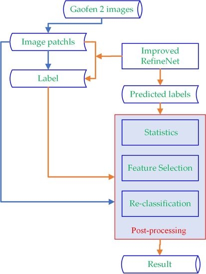
2. Study Area and Data

2.1. Study Area

Feicheng is a county-level city covering 1277 km² in central-western Shandong Province, China (35°53′ to 36°19′N, 116°28′ to 116°59′E; Figure 1). This is an important Chinese production area for commodity grains such as winter wheat (the main local crop). The area has a warm temperate continental sub-humid monsoon climate with four distinct seasons; the average annual precipitation is 645.7 mm, the average annual temperature is 13.6 °C, and the average annual sunshine duration is 2281.3 h. Feicheng’s variable terrain includes mountains along its northern border and central hills, separated by several plains and rivers; its landscape and climate are representative of many Chinese regions, making it an appropriate study area for our purposes.

2.2. Remote Sensing Imagery

We collected 63 Gaofen-2 (GF-2) remote sensing images as experimental data: 19 from 2017, 23 from 2018, and 21 from 2019. Each image contained multi-spectral bands (blue, green, red, and near-infrared) with 4-m resolution and panchromatic bands with 1-m resolution. After mosaicking, the images from each year covered Feicheng completely. As winter wheat has distinct characteristics during winter, all images were chosen during that time to improve the accuracy of the extraction results.

We used Environment for Visualizing Images (ENVI) software to conduct four pre-processing steps for all images. First, multi-spectral and panchromatic orthographic correction was completed using measured ground control points and the rational polynomial coefficient (RPC) model, based on 30-m resolution DEM data from the Shuttle Radar Topography Mission (https://earthexplorer.usgs.gov/).

Second, radiometric calibration involved calibrating the multi-spectral data from the original digital number (DN) value to the equivalent radiance by:

$$l=DN*g+b,$$

(1)

where l is the equivalent radiance obtained after conversion, DN is the DN value of the pixel, g is the calibration coefficient, and b is the calibration offset; both g and b were published by the China Resource Satellite Application Center (http://www.cresda.com/cn/).

Third, atmospheric correction used the Fast Line-of-sight Atmospheric Analysis of Hypercubes (FLAASH) module in ENVI. Given the acquisition season, latitude, and land cover, the Sub-Arctic Summer model was adopted for the atmospheric model and the Rural model was adopted for the aerosol model; the initial visibility was 40 km.

Fourth, fusion processing of the panchromatic and multi-spectral data used the Gram-Schmidt Pan Sharpening module in ENVI. After fusion, the spatial resolution of the resulting image was 1 m with the red, blue, green, and near-infrared bands; each image was 7300 × 6900 pixels.

2.3. Ground Survey Data

The main land-use types in the study area during winter include winter wheat, buildings, roads, woodland, water bodies, agricultural buildings, unplanted farmland, and other. In the GF-2 imagery, buildings, roads, water bodies, agricultural buildings, unplanted farmland, and other all have obvious color and texture features that can be easily distinguished visually. However, winter wheat and woodland (especially some evergreen trees) are more similar in color and texture. To address this, we conducted ground investigations throughout the study area from December 2017 to January 2019, obtaining 119 samples (83 winter wheat and 36 woodland) for which the coordinates, type, and other information were recorded, along with photos (Figure 2).

2.4. Labeled Image Dataset

We selected 317 non-overlapping 960×720-pixel sub-regions within the fused image (Section 2.2), then labeled each manually. After labeling was completed, each sub-region corresponded to a label file, forming an image–label pair (Figure 3). These files were single-band files in which the number of pixel rows and columns was consistent with the corresponding image. Each labeled pixel was given a category number: winter wheat (1), buildings (2), roads (3), water bodies (4), agricultural buildings (5), unplanted farmland (6), woodland (7), and other (8).

3. Method

Our method consisted of three steps. First, the improved RefineNet generated the initial segmentation and outputted a category probability vector for each pixel (Section 3.1). Second, these initial segmentations were statistically analyzed using manual labels as a reference to determine the confidence threshold (Section 3.2). Third, all pixels below the confidence threshold were post-processed to generate their final category label (Section 3.3).

3.1. Initial Segmentation by CNN

In the common CNN structure, the feature extractor comprises multiple overlapping convolutional layers, each of which was followed by pooling, batch normalization, and activation layers (Figure 4). The convolution layer contained several convolution kernels, most of which were 3 × 3. The pooling layer aggregated the features, which was beneficial for screening out features with good discrimination. The batch normalization layer was used to normalize the feature values. The activation layer adopted a nonlinear function. According to Hornik [70], the use of an activation layer facilitates better expressions of the correlation features between similar pixels and better optimization of features.

The feature vector generator is generally composed of deconvolution layers, which can generate feature vectors of equal length for each pixel. These generated feature vectors are used as the inputs for the classifier to determine the pixel category. Therefore, the deconvolution performance directly determines the model performance. At present, most CNNs used for image segmentation have similar feature extractor structures; they are mainly distinguished by their feature vector generators. For example, FCN uses the interpolation method as a feature vector generator, while SegNet uses the deconvolution kernel. More recent CNNs generate pixel-level feature vectors using trained deconvolution kernels.

Unlike other CNNs, RefineNet [42] uses a new “multipath” structure to fuse fine low-level features and rough high-level features, effectively improving the distinguishability of features and greatly improving the accuracy of segmentation results. The RefineNet feature vector generator consists of four levels. Each level uses the results of both the higher-level semantic feature deconvolution and the feature extractor at the same level as the input. This multi-level feature fusion strategy improves the distinguishability of features.

Considering the superior performance of the RefineNet model, we chose this as the initial segmentation model in our study. Similar to other CNNs, RefineNet also employs the Softmax model as a classifier.

We used a modified Softmax model as a classifier. The modified SoftMax model also takes a pixel-level feature vector as the input, and calculates the probability of classifying the pixel into each category. The category corresponding to the maximum probability value was assigned as the category of the pixel. The probabilities were organized into a category probability vector. The output included the category probability vector and initial category for each pixel.

3.2. Statistics for Initial Classification Results

Statistical analysis showed that the most pixels which had been correctly classified were located inside the winter wheat planting area, and the most pixels which had been incorrectly classified were located at the edge of this area. Statistical analysis also showed that the difference between the maximum probability value and the second-highest probability value was generally large in the category probability vectors of pixels that had been correctly classified, but that it was generally small or nearly equivalent in the category probability vectors of pixels that had been incorrectly classified.

We proposed the confidence level (CL) as an indicator for the credibility of the CNN segmentation results. The CL of a category probability vector was calculated as:

$$CL=p_i-p_j,$$

(2)

where p is a category probability vector, $p_i$ is the maximum value in p, and $p_j$ is the second-highest value in p.

Our analysis showed that the classification result for a pixel could be considered credible if the CL of this pixel was higher than the minimum confidence threshold (minCL); otherwise, it was considered non-credible. Those pixels with CL values lower than minCL required post-processing. In our study, based on the statistical analysis of the training results, 0.21 was selected as minCL.

3.3. Low-Confidence Pixel Post-Processing

3.3.1. Feature Selection

Based on the prior knowledge that the inner pixels and edge pixels in winter wheat planting areas have very similar colors and textures, and the near-infrared (NIR) band is sensitive to crops, we created a feature vector for each pixel using the red, blue, green, and near-infrared bands along with NDVI, uniformity (UNI), contrast (CON), entropy (ENT), and inverse difference (INV). NDVI was calculated following Wang et al. [10],

$$NDVI=\frac{NIR-Red}{NIR+Red},$$

(3)

UNI, CON, ENT, and INV were extracted using the methods proposed by Yang and Yang, based on GLCM [23],

$$UNI={{\displaystyle \sum }}_{i=1}^q{{\displaystyle \sum }}_{j=1}^q{\left(g\left(i,j\right)\right)}^2,$$

(4)

$$CON={{\displaystyle \sum }}_{n=0}^{q-1}{n}^2\left\{{{\displaystyle \sum }}_{i=1}^q{{\displaystyle \sum }}_{j=1}^{q}g\left(i,j\right)\right\}where\left|i-j\right|=n,$$

(5)

$$ENT=-{{\displaystyle \sum }}_{i=1}^q{{\displaystyle \sum }}_{j=1}^q(g\left(i,j\right)\log \left\{g\left(i,j\right)\right\},$$

(6)

$$INV={{\displaystyle \sum }}_{i=1}^q{{\displaystyle \sum }}_{j=1}^q\frac{g\left(i,j\right)}{1+{\left(i-j\right)}^2},$$

(7)

In (4)–(7), q is the gray level quantization and g(i,j) is the element of GLCM.

The feature vector v of each pixel had nine elements, structured as:

$$v=(red,green,blue,NIR,NDVI,UNI,CON,ENT,INV)$$

(8)

3.3.2. Vector Distance Calculation Method

We used the improved Euclidean distance to calculate the vector distance of the two feature vectors. The standard Euclidean distance is defined as:

$$d\left(x,y\right)=\sqrt{{{\displaystyle \sum }}_{i=1}^b(x_i-y_i{)}^2},$$

(9)

where x and y are the feature vectors to be compared, x_i and y_i are the feature components, and b is the length of the feature vector. Smaller distances between the two feature vectors correspond to greater similarity. In the standard Euclidean distance, all elements are considered to have equal weight, without considering the influence of the aggregation degree of elements on the distance.

Statistically, among the features of the samples of the same category, a higher concentration of the value of a certain feature corresponds to stronger distinguishability of this feature and greater weight that should be assigned to this feature. Similarly, greater dispersion in the value of a certain feature corresponds to weaker distinguishability and smaller assigned weight of this feature.

Based on prior knowledge, we introduced the reciprocal of the feature value distance as the weight factor to improve the Euclidean distance, thus better reflecting the influence of feature value aggregation on the vector distance. This weight factor was calculated as:

$$w_i=\frac{1}{\left|ma{x}_i-mi{n}_i\right|},$$

(10)

where i is the position number of the component in the feature vector, w_i is the weight of the component, max_i is the maximum value of the ith components of all feature vectors, and min_i is the minimum value of the ith components of all feature vectors. On this basis, the vector distance calculation formula was:

$$d\left(x,y\right)=\sqrt{{{\displaystyle \sum }}_{i=1}^n{w}_i(x_i-y_i{)}^2},$$

(11)

where x and y are the feature vectors to be compared, x_i and y_i are the feature components, w_i is the weight of component i, and n is the component number of the feature vector.

3.3.3. Vector Distance Threshold Determination

• Firstly, each complete crop planting area in the training image was set as a statistical unit. The vector distance d between each pixel and other pixels was calculated individually, and the maximum vector distance d_i of the unit was recorded, where i was the number of the statistical unit.
• Secondly, the vector distance threshold (vdt) was obtained by:

  $$vdt=\underset{1\le i\ll n}{\max }{d}_i,$$

  (12)

  where n is the number of statistical units.

3.3.4. Low-confidence Pixel Classification

We used the following steps to optimize the results of winter wheat planting areas outputted by the improved RefineNet model:

• NDVI for each pixel was calculated;
• UNI, CON, ENT, and INV for each pixel was calculated;
• CL was calculated pixel by pixel;
• Winter wheat pixels with continuous position and CL > minCL were divided into a separate group;
• For each group, the adjacent pixels for which CL < minCL were processed individually. For a certain adjacent pixel p, we calculated the vector distances between p and each pixel in the adjacent group and then chose the minimum value as the minimum distance mind. If mind < vdt, p was re-classified as a winter wheat pixel.

3.4. Experimental Setup

We conducted a comparative experiment on a graphics workstation with a 12-GB internal graphics card and a Linux Ubuntu 16.04 operating system. TensorFlow 1.10 software was used to write the statistical analysis and post-processing code in the Python language. Using a RefineNet model from the GitHub platform, we modified the output of the SoftMax model used by RefineNet. We used this for initial segmentation and used the output as basic data for statistical analysis.

We selected the SegNet and unmodified RefineNet models as standard CNN and CRF as the post-process method for comparison with PP-CNN (

Table 1. Models used in the comparative experiment.

Name	Description
PP-CNN	The proposed method
SegNet	Classifier using only high-level semantic features
SegNet-CRF	SegNet was used as the initial segmentation model, CRF was used as the post-processing method
PP-SegNet	As in PP-CNN, SegNet was used as the initial segmentation model
RefineNet	Linear model was adopted for feature fusion
RefineNet-CRF	Classic RefineNet was used as the initial segmentation model, CRF was used as the post-processing method

). SegNet works like RefineNet, except it uses only high-level semantic features to generate feature vectors for each pixel.

By comparing the results from SegNet and RefineNet, we hoped to verify that the strategy of generating features with RefineNet was better than that of generating features with SegNet. By comparing the results of SegNet-CRF, RefineNet, and RefineNet-CRF with PP-CNN, we hoped to show that post-processing could effectively improve the accuracy of segmentation results. By comparing the results of SegNet with PP-SegNet, we hoped to show that the proposed post-processing method had strong adaptability.

We applied data augmentation techniques onto the training dataset, including horizontal flip, color adjustment, and vertical flip steps. The color adjustment factors used included brightness, hue, saturation, and contrast. Each image in the training dataset was processed 10 times. All images created by the data augmentation techniques were only used in training the CNNs.

We used cross-validation techniques in the comparative experiments. Each CNN model was trained over four rounds; in each round, 87 images were selected as test images and the other images were used as training images. Each image was used at least once as the test image (

Table 2. Percent of every category sample used in experiments.

Category	Percent of Total Samples
Winter wheat	39.00%
Agricultural buildings	0.10%
Woodland	9.01%
Buildings	19.01%
Roads	0.81%
Water bodies	0.90%
Unplanted farmland	24.12%
Other	7.05%

).

Table 3. The hyper-parameter setup.

Hyper-Parameter	Value
mini-batch size	32
learning rate	0.0001
momentum	0.9
epochs	20000

shows the hyper-parameter setup we used to train our model. In the comparison experiments, the hyper-parameters were also applied to the comparison model.

4. Results

We randomly selected ten test images from the test data set and assessed their segmentation results using the SegNet, SegNet-CRF, PP-SegNet, RefineNet, RefineNet-CRF, and PP-CNN models (Figure 5).

The six methods had very similar performances within the winter wheat planting areas, with virtually no misclassifications. However, differences were obvious at the edges of these areas. PP-CNN and PP-SegNet misclassified only very small numbers of discrete pixels, while SegNet had the most errors in a more continuous pattern, with errors being more common at corners than at edges. RefineNet had significantly fewer errors than the SegNet model, with most located near corners and few in continuous patterns.

Comparing SegNet-CRF and PP-SegNet, RefineNet, and PP-CNN, respectively, it can be seen that, on the premise that the initial segmentation results are the same, the results obtained by post-processing using the proposed method are better than those obtained by using CRF. Considering that CRF has very good performance in processing camera images, this may be because the resolution of remote sensing images is lower than that of camera images, which reduces the performance of CRF. It shows that the appropriate post-processing method should be selected according to the image characteristics.

Whether using CRF or the method proposed in this paper, the accuracy of the results after post-processing is improved, which also shows the importance of post-processing methods when CNN is applied to image segmentation.

We then produced a confusion matrix for the segmentation results for all four methods (

Table 4. Confusion matrix for winter wheat classification.

Approach	Predicted	Winter Wheat	Non-Winter Wheat
SegNet	Winter wheat	29.6%	9.4%
	Non-winter wheat	9.9%	51.1%
SegNet-CRF	Winter wheat	31.9%	7.1%
	Non-winter wheat	8.3%	52.7%
PP-SegNet	Winter wheat	33.1%	5.9%
	Non-winter wheat	5.9%	55.1%
RefineNet	Winter wheat	32.5%	6.5%
	Non-winter wheat	6.3%	54.7%
RefineNet-CRF	Winter wheat	35.3%	3.7%
	Non-winter wheat	7.8%	53.2%
PP-CNN	Winter wheat	36.9%	2.1%
	Non-winter wheat	3.5%	57.5%

), where each column represents the classification result obtained from the segmentation results and each row represents the actual category defined by manual classification. PP-CNN was clearly superior, with classification errors accounting for only 5.6%, lower than the 13.7% for SegNet, 9.8% for SegNet-CRF, 6.2% for PP-SegNet, 7.2% for RefineNet, and 5.9% for RefineNet-CRF.

We used the accuracy, precision, recall, and Kappa coefficient to evaluate the performance of the four models [45] (

Table 5. Statistical comparison of model performance.

Index	SegNet	SegNet-CRF	PP-SegNet	RefineNet	RefineNet-CRF	PP-CNN
Accuracy	80.7%	84.6%	88.2%	87.2%	88.5%	94.4%
Precision	79.7%	83.7%	87.6%	86.6%	87.7%	93.9%
Recall	79.8%	84.1%	87.6%	86.5%	88.9%	94.4%
Kappa	0.663	0.722	0.779	0.763	0.786	0.889

). The average accuracy of PP-CNN was 13.7% higher than SegNet, 7.2% higher than RefineNet, and 6.2% higher than PP-SegNet.

Table 6. Statistical comparison of model performance.

Index	SegNet	SegNet-CRF	PP-SegNet	RefineNet	RefineNet-CRF	PP-CNN
Time [ms]	295	375	301	297	361	302

*ms: millisecond

shows the average time required for each method to complete the testing of one image. The proposed post-processing method requires an approximate increase of 2% in time and improves the accuracy by 7.2%. The time consumed by CRF is higher than that consumed by the proposed method because the CRF must calculate the distances between all pixel–pixel pairs for a single image, while the proposed method must calculate the distances for only a small number of pixel–pixel pairs.

5. Discussion

5.1. Advantages of PP-CNN

When an image is segmented pixel-wise by a CNN, the accuracy of the results is determined by the feature extractor, feature generator, and classifier. The first two use trained feature extraction rules to process remote sensing images and obtain feature vectors for each pixel, while the third uses trained classification rules to process the acquired feature vectors and determine the pixel category. Therefore, both sets of rules aim to express the main common features of similar objects. In remote sensing images, the number of inner pixels for most objects is much larger than the number of edge pixels, such that the trained rules tend to reflect the inner features, making classification errors more likely at the edge of the object.

In order to further illustrate the influence of pixel position on feature extraction, we defined the pixel blocks used to calculate feature values as three types: internal (type A), in which the pixel blocks used are all composed of the same kind of pixel; edge (type B), in which the pixel blocks used contain ~50% of other types of pixel; and corner (type C), in which the pixel blocks used contain 75% or more of other categories of pixel (Figure 6). Considering that CNNs use the same convolution kernel for feature extraction, it is clear that when the channel values of other categories of pixels in the calculated pixel blocks are different from the category of interest, the feature values of pixels in types A, B, and C will be quite different. Especially for type C pixels, if the difference between the pixel value and the neighboring pixel value is large, the calculated feature value may be closer to the feature value range of the neighboring category. This makes it difficult to effectively solve the problem of higher error occurrence in edge pixel segmentation simply by using a CNN.

Statistical analysis showed that, although crop planting areas may have clear differences between inner and edge pixels in high-level semantic features, these remain quite similar in low-level features (such as color or texture). Considering the high accuracy of inner pixel classification in our extraction results, PP-CNN clearly integrated the advantages of CNNs and statistical features, thus significantly improving the accuracy of the extraction results.

5.2. Influence of Maximum Vector Distance Threshold on PP-CNN Segmentation Results

The PP-CNN method uses color, texture, and other features to compose feature vectors and combines statistical analysis techniques to post-process the results of the CNN model, thereby providing improved spatial distribution data for winter wheat. When performing post-processing, we first calculated the vector distance between low-confidence pixels and nearby crop pixels with high confidence. We then compared the obtained vector distance with the vector distance threshold obtained by statistical analysis to determine whether low-confidence pixels could be classified as winter wheat. We took the maximum vector distance calculated by all statistical units as the vector distance threshold.

To compare the impact of vector distance thresholds on model performance, we used the minimum vector distance (method I), the average of all vector distances (method II), and the maximum vector distance (method III) as the vector distance threshold, respectively, with the results shown in

Table 7. Comparison of PP-CNN model performance for minimum (I), average (II), and maximum (III) vector distances.

Index	I	II	III
Precision	96.1%	94.8%	93.9%
Recall	90.1%	92.5%	94.4%

.

Method III had the lowest precision but the highest recall rate, because using the maximum distance as the threshold means that similar pixels of other categories are classified as winter what pixels, thus reducing the accuracy. However, method I ensures maximum winter pixel extraction. Therefore, when PP-CNN is applied in the real world, researchers should choose among the three methods according to the extraction target and research goals.

5.3. Influence of Feature Strategy on Classification Results

We further compared SegNet and RefineNET by analyzing the impact of feature extraction strategies on the classification results. We selected a group of semantic features from the last layer of the SegNet and RefineNet models having the greatest difference. We divided these features into three groups of pixels: winter wheat edge, winter wheat inner, and non-winter wheat (Figure 7). Here, “inner” meant that when extracting the pixel features, only the winter wheat pixels included in the pixel block participated in the feature calculation; “edge” meant that pixels mixed with other categories participated. The feature results extracted by RefineNet were more concentrated by type and better discriminated between type; in comparison, the SegNet results were far less coherent. The feature fusion strategy adopted by the RefineNet model was clearly more conducive to improving the accuracy of the results than SegNet’s strategy of only using high-level semantic features.

6. Conclusions

Using CNNs to extract crop spatial distribution information from satellite remote sensing imagery has become increasingly common. However, the use of CNNs alone usually results in very rough edge areas, with a corresponding negative influence on overall accuracy. We used prior knowledge and statistical analysis to optimize winter wheat CNN extraction results, especially with regard to edge areas.

We analyzed the root cause of increased errors in CNN edge pixel classification, then used the category probability vector output to calculate the results’ credibility, dividing these into high-credibility and low-credibility pixels for subsequent processing. We then optimized the accuracy of the latter’s classification by analyzing the characteristics of planting area pixels using prior knowledge of the segmentation results. This new extraction strategy effectively improved the accuracy of crop extraction results.

Although the PP-CNN post-processing method proposed here was mainly established for crop extraction, it could be applied to the extraction of water, forest, grassland, and other land-use types with small internal pixel differences. However, for land-use types with larger internal differences, such as residential land, other post-treatment feature organization methods must be developed. The main disadvantage of our approach is the need for more manually classified images; future research should test the use of semi-supervised classification to reduce this dependence.

References

1. Atzberger, C. Advances in remote sensing of agriculture: Context description, existing operational monitoring systems and major information needs. Remote Sens. 2013, 5, 949–981. [Google Scholar] [CrossRef] [Green Version]
2. Zhang, J.; Feng, L.; Yao, F. Improved maize cultivated area estimation over a large scale combining MODIS–EVI time series data and crop phenological information. ISPRS J. Photogramm. Remote Sens. 2014, 94, 102–113. [Google Scholar] [CrossRef]
3. Mhangara, P.; Odindi, J. Potential of texture-based classification in urban landscapes using multispectral aerial photos. S. Afr. J. Sci. 2013, 109, 1–8. [Google Scholar] [CrossRef] [Green Version]
4. Wang, F.; Kerekes, J.P.; Xu, Z.Y.; Wang, Y.D. Residential roof condition assessment system using deep learning. J. Appl. Remote Sens. 2018, 12, 016040. [Google Scholar] [CrossRef] [Green Version]
5. Jiang, T.; Liu, X.N.; Wu, L. Method for mapping rice fields in complex landscape areas based on pre-trained convolutional neural network from HJ-1 A/B data. ISPRS Int. J. Geo Inf. 2018, 7, 418. [Google Scholar] [CrossRef] [Green Version]
6. El-naggar, A.M. Determination of optimum segmentation parameter values for extracting building from remote sensing images. Alex. Eng. J. 2018, 57, 3089–3097. [Google Scholar] [CrossRef]
7. Zhang, B.; Liu, Y.Y.; Zhang, Z.Y.; Shen, Y.L. Land use and land cover classification for rural residential areas in China using soft-probability cascading of multifeatures. J. Appl. Remote Sens. 2017, 11, 045010. [Google Scholar] [CrossRef] [Green Version]
8. Younes, N.; Joyce, K.E.; Northfield, T.D.; Maier, S.W. The effects of water depth on estimating Fractional Vegetation Cover in mangrove forests. Int. J. Appl. Earth Obs. Geoinf. 2019, 83, 101924. [Google Scholar] [CrossRef]
9. Blaschke, T.; Feizizadeh, B.; Hölbling, D. Object-based image analysis and digital terrain analysis for locating landslides in the Urmia Lake Basin, Iran. IEEE J. Select. Top. Appl. Earth Obs. Remote Sens. 2014, 7, 4806–4817. [Google Scholar] [CrossRef]
10. Wang, L.; Chang, Q.; Yang, J.; Zhang, X.H.; Li, F. Estimation of paddy rice leaf area index using machine learning methods based on hyperspectral data from multi-year experiments. PLoS ONE 2018, 13, e0207624. [Google Scholar] [CrossRef] [Green Version]
11. Feyisa, G.L.; Meilby, H.; Fensholt, R.; Proud, S.R. Automated Water Extraction Index: A new technique for surface water mapping using Landsat imagery. Remote Sens. Environ. 2014, 140, 23–35. [Google Scholar] [CrossRef]
12. Bhatti, S.S.; Tripathi, N.K. Built-up area extraction using Landsat 8 OLI imagery. GISci. Remote Sens. 2014, 51, 445–467. [Google Scholar] [CrossRef] [Green Version]
13. Xu, H.Q. A remote sensing index for assessment of regional ecological changes. China Environ. Sci. 2013, 33, 889–897. [Google Scholar] [CrossRef]
14. Wang, W.J.; Zhang, X.; Zhao, Y.D.; Wang, S.D. Cotton extraction method of integrated multi-features based on multi-temporal Landsat 8 images. J. Remote Sens. 2017, 21, 115–124. [Google Scholar] [CrossRef]
15. Kussul, N.; Lavreniuk, M.; Skakun, S.; Shelestov, A. Deep learning classification of land cover and crop types using remote sensing data. IEEE Geosci. Remote Sens. Lett. 2017, 14, 778–782. [Google Scholar] [CrossRef]
16. Beyer, F.; Jarmer, T.; Siegmann, B. Identification of agricultural crop types in northern Israel using multitemporal RapidEye data. Photogramm. Fernerkund. Geoinf. 2015, 2015, 21–32. [Google Scholar] [CrossRef]
17. Warner, T.A.; Steinmaus, K. Spatial classification of orchards and vineyards with high spatial resolution panchromatic imagery. Photogramm. Eng. Remote Sens. 2005, 71, 179–187. [Google Scholar] [CrossRef]
18. Li, L.; Liang, J.; Weng, M.; Zhu, H. A multiple-feature reuse network to extract buildings from remote sensing imagery. Remote Sens. 2018, 10, 1350. [Google Scholar] [CrossRef] [Green Version]
19. Reis, S.; Taşdemir, K. Identification of hazelnut fields using spectral and Gabor textural features. ISPRS J. Photogramm. Remote Sens. 2011, 66, 652–661. [Google Scholar] [CrossRef]
20. Moya, L.; Zakeri, H.; Yamazaki, F.; Liu, W.; Mas, E.; Koshimura, S. 3D gray level co-occurrence matrix and its application to identifying collapsed buildings. ISPRS J. Photogramm. Remote Sens. 2019, 149, 14–28. [Google Scholar] [CrossRef]
21. Chen, J.; Deng, M.; Xiao, P.F.; Yang, M.H.; Mei, X.M. Rough set theory based object-oriented classification of high resolution remotely sensed imagery. J. Remote Sens. 2010, 14, 1139–1155. [Google Scholar] [CrossRef]
22. Zhao, Y.D.; Zhang, L.P.; Li, P.X. Universal Markov random fields and its application in multispectral textured image classification. J. Remote Sens. 2006, 10, 123–129. [Google Scholar] [CrossRef]
23. Yang, P.; Yang, G. Feature extraction using dual-tree complex wavelet transform and gray level co-occurrence matrix. Neurocomputing 2016, 197, 212–220. [Google Scholar] [CrossRef]
24. Mao, L.; Zhang, G.M. Complex cue visual attention model for harbor detection in high-resolution remote sensing images. J. Remote Sens. 2017, 21, 300–309. [Google Scholar] [CrossRef]
25. Liu, P.H.; Liu, X.P.; Liu, M.X.; Shi, Q.; Yang, J.X.; Xu, X.C.; Zhang, Y.Y. Building footprint extraction from high-resolution images via spatial residual inception convolutional neural network. Remote Sens. 2019, 11, 830. [Google Scholar] [CrossRef] [Green Version]
26. Kim, S.; Son, W.J.; Kim, S.H. Double weight-based SAR and infrared sensor fusion for automatic ground target recognition with deep learning. Remote Sens. 2018, 10, 72. [Google Scholar] [CrossRef] [Green Version]
27. Gao, J.; Wang, K.; Tian, X.Y.; Chen, J. A BP-NN Based Cloud Detection Method For FY-4 Remote Sensing images. J. Infrared Millim. Waves 2018, 37, 477–485. [Google Scholar] [CrossRef]
28. Li, X.; Lyu, X.; Tong, Y.; Li, S.; Liu, D. An object-based river extraction method via Optimized Transductive Support Vector Machine for multi-spectral remote-sensing images. IEEE Access 2019, 7, 46165–46175. [Google Scholar] [CrossRef]
29. He, T.; Sun, Y.J.; Xu, J.D.; Wang, X.J.; Hu, C.R. Enhanced land use/cover classification using support vector machines and fuzzy k-means clustering algorithms. J. Appl. Remote Sens. 2014, 8, 083636. [Google Scholar] [CrossRef] [Green Version]
30. Zhang, K.W.; Hu, B.X. Individual urban tree species classification using very high spatial resolution airborne multi-spectral imagery using longitudinal profiles. Remote Sens. 2012, 4, 1741–1757. [Google Scholar] [CrossRef] [Green Version]
31. Sang, X.; Guo, Q.Z.; Wu, X.X.; Fu, Y.; Xie, T.Y.; He, C.W.; Zang, J.L. Intensity and stationarity analysis of land use change based on CART algorithm. Nat. Sci. Rep. 2019, 9, 12279. [Google Scholar] [CrossRef] [PubMed] [Green Version]
32. Santos Pereira, L.F.; Barbon, S.; Valous, N.A.; Barbin, D.F. Predicting the ripening of papaya fruit with digital imaging and random forests. Comput. Electron. Agric. 2018, 145, 76–82. [Google Scholar] [CrossRef]
33. Wang, N.; Li, Q.Z.; Du, X.; Zhang, Y.; Zhao, L.C.; Wang, H.Y. Identification of main crops based on the univariate feature selection in Subei. J. Remote Sens. 2017, 21, 519–530. [Google Scholar] [CrossRef]
34. Krizhevsky, A.; Sutskever, I.; Hinton, G. ImageNet classification with deep convolutional neural networks. Commun. ACM 2017, 60, 84–90. [Google Scholar] [CrossRef]
35. Szegedy, C.; Liu, W.; Jia, Y.Q.; Sermanet, P.; Reed, S.; Anguelov, D.; Erhan, D.; Vanhoucke, V.; Rabinovich, A. Going deeper with convolutions. In Proceedings of the 2015 IEEE Conference on Computer Vision and Pattern Recognition, Boston, MA, USA, 7–12 June 2015. [Google Scholar] [CrossRef]
36. Simonyan, K.; Zisserman, A. Very deep convolutional networks for large-scale image recognition. arXiv 2014, arXiv:1409.1556. [Google Scholar]
37. He, K.M.; Zhang, X.Y.; Ren, S.Q.; Sun, J. Deep residual learning for image recognition. In Proceedings of the 2016 IEEE Conference on Computer Vision and Pattern Recognition, Las Vegas, NV, USA, 27–30 June 2016. [Google Scholar] [CrossRef] [Green Version]
38. Long, J.; Shelhamer, E.; Darrell, T. Fully convolutional networks for semantic segmentation. In Proceedings of the 2015 IEEE Conference on Computer Vision and Pattern Recognition, Boston, MA, USA, 7–12 June 2015. [Google Scholar] [CrossRef] [Green Version]
39. Badrinarayanan, V.; Kendall, A.; Cipolla, R. SegNet: A deep convolutional encoder-decoder architecture for image segmentation. IEEE Trans. Pattern Anal. Mach. Intell. 2017, 39, 2481–2495. [Google Scholar] [CrossRef]
40. Chen, L.C.; Papandreou, G.; Kokkinos, I.; Murphy, K.; Yuille, A.L. DeepLab: Semantic image segmentation with deep convolutional nets, Atrous convolution, and fully connected CRFs. IEEE Trans. Pattern Anal. Mach. Intell. 2018, 40, 834–848. [Google Scholar] [CrossRef]
41. Lin, G.S.; Milan, A.; Shen, C.H.; Reid, I. RefineNet: Multi-path refinement networks for high-resolution semantic segmentation. In Proceedings of the 2017 IEEE Conference on Computer Vision and Pattern Recognition, Honolulu, HI, USA, 21–26 July 2017. [Google Scholar] [CrossRef] [Green Version]
42. Ronneberger, O.; Fischer, P.; Brox, T. U-Net: Convolutional networks for biomedical image segmentation. In Medical Image Computing and Computer-Assisted Intervention—MICCAI 2015; Lecture Notes in Computer Science; Navab, N., Hornegger, J., Wells, W., Frangi, A., Eds.; Springer: Berlin, Germany, 2015; Volume 9351. [Google Scholar] [CrossRef] [Green Version]
43. Cui, W.; Wang, F.; He, X.; Zhang, D.Y.; Xu, X.X.; Yao, M.; Wang, Z.W. Multi-scale semantic segmentation and spatial relationship recognition of remote sensing images based on an attention model. Remote Sens. 2019, 11, 1044. [Google Scholar] [CrossRef] [Green Version]
44. Fu, G.; Liu, C.J.; Zhou, R.; Sun, T.; Zhang, Q.J. Classification for high resolution remote sensing imagery using a fully convolutional network. Remote Sens. 2017, 9, 498. [Google Scholar] [CrossRef] [Green Version]
45. Lu, J.Y.; Wang, Y.Z.; Zhu, Y.Q.; Ji, X.H.; Xing, Y.T.; Li, W.; Zomaya, A.Y. P_segnet and NP_segnet: New neural network architectures for cloud recognition of remote sensing images. IEEE Access 2019, 7, 87323–87333. [Google Scholar] [CrossRef]
46. Shustanov, A.; Yakimov, P. CNN design for real-time traffic sign recognition. Procedia Eng. 2017, 201, 718–725. [Google Scholar] [CrossRef]
47. Dai, X.B.; Duan, Y.X.; Hu, J.P.; Liu, S.C.; Hu, C.Q.; He, Y.Z.; Chen, D.P.; Luo, C.L.; Meng, J.Q. Near infrared nighttime road pedestrians recognition based on convolutional neural network. Infrared Phys. Technol. 2019, 97, 25–32. [Google Scholar] [CrossRef]
48. Wang, D.D.; He, D.J. Recognition of apple targets before fruits thinning by robot based on R-FCN deep convolution neural network. Trans. Chin. Soc. Agric. Eng. 2019, 35, 156–163. [Google Scholar] [CrossRef]
49. Ferentinos, K.P. Deep learning models for plant disease detection and diagnosis. Comput. Electron. Agric. 2018, 145, 311–318. [Google Scholar] [CrossRef]
50. Cheng, X.; Zhang, Y.H.; Chen, Y.Q.; Wu, Y.Z.; Yue, Y. Pest identification via deep residual learning in complex background. Comput. Electron. Agric. 2017, 141, 351–356. [Google Scholar] [CrossRef]
51. Liu, F.; Shen, T.; Ma, X.; Zhang, J. Ship recognition based on multi-band deep neural network. Opt. Precis. Eng. 2017, 25, 166–173. [Google Scholar] [CrossRef]
52. Chen, Y.; Zhang, C.M.; Wang, S.Y.; Li, J.P.; Li, F.; Yang, X.X.; Wang, Y.Y.; Yin, L.K. Extracting crop spatial distribution from Gaofen 2 imagery using a convolutional neural network. Appl. Sci. 2019, 9, 2917. [Google Scholar] [CrossRef] [Green Version]
53. Xie, B.; Zhang, H.K.; Xue, J. Deep convolutional neural network for mapping smallholder agriculture using high spatial resolution satellite image. Sensors 2019, 19, 2398. [Google Scholar] [CrossRef] [Green Version]
54. Yang, W.; Yang, C.; Hao, Z.Y.; Xie, C.Q.; Li, M.Z. Diagnosis of plant cold damage based on hyperspectral imaging and convolutional neural network. IEEE Access 2019, 7, 118239–118248. [Google Scholar] [CrossRef]
55. Li, Y.; Zhang, H.; Shen, Q. Spectral–spatial classification of hyperspectral imagery with 3D convolutional neural network. Remote Sens. 2017, 9, 67. [Google Scholar] [CrossRef] [Green Version]
56. Sellami, A.; Farah, M.; Farah, I.R.; Solaiman, B. Hyperspectral imagery classification based on semi-supervised 3-D deep neural network and adaptive band selection. Expert Syst. Appl. 2019, 129, 246–259. [Google Scholar] [CrossRef]
57. Alonzo, M.; Andersen, H.E.; Morton, D.C.; Cook, B.D. Quantifying boreal forest structure and composition using UAV structure from motion. Forests 2018, 9, 119. [Google Scholar] [CrossRef] [Green Version]
58. Zhang, C.; Pan, X.; Li, H.; Gardiner, A.; Sargent, I.; Hare, J.; Atkinson, P.M. A hybrid MLP-CNN classifier for very fine resolution remotely sensed image classification. ISPRS J. Photogramm. Remote Sens. 2018, 140, 133–144. [Google Scholar] [CrossRef] [Green Version]
59. Jozdani, S.E.; Johnson, B.A.; Chen, D. Comparing deep neural networks, ensemble classifiers, and support vector machine algorithms for object-based urban land use/land cover classification. Remote Sens. 2019, 11, 1713. [Google Scholar] [CrossRef] [Green Version]
60. Carranza-García, M.; García-Gutiérrez, J.; Riquelme, J.C. A framework for evaluating land use and land cover classification using convolutional neural networks. Remote Sens. 2019, 11, 274. [Google Scholar] [CrossRef] [Green Version]
61. Zhang, C.M.; Han, Y.J.; Li, F.; Gao, S.; Song, D.J.; Zhao, H.; Fan, K.Q.; Zhang, Y.N. A new CNN-Bayesian model for extracting improved winter wheat spatial distribution from GF-2 imagery. Remote Sens. 2019, 11, 619. [Google Scholar] [CrossRef] [Green Version]
62. Zheng, S.; Jayasumana, S.; Romera-Paredes, B.; Vineet, V.; Su, Z.; Du, D.; Huang, C.; Torr, P.H. Conditional random fields as recurrent neural networks. In Proceedings of the 2015 IEEE International Conference on Computer Vision (ICCV), Santiago, Chile, 7–13 December 2015; pp. 1529–1537. [Google Scholar]
63. Teichmann, M.T.T.; Cipolla, R. Convolutional CRFs for Semantic Segmentation. arXiv 2018, arXiv:1805.04777. [Google Scholar]
64. Audebert, N.; Boulch, A.; Saux, B.E.; Lefèvre, S. Distance transform regression for spatially-aware deep semantic segmentation. Comput. Vis. Image Underst. 2019, 189, 102809. [Google Scholar] [CrossRef] [Green Version]
65. Fu, T.; Ma, L.; Li, M.; Johnson, B.A. Using convolutional neural network to identify irregular segmentation objects from very high-resolution remote sensing imagery. J. Appl. Remote Sens. 2018, 12, 025010. [Google Scholar] [CrossRef]
66. Mboga, N.; Georganos, S.; Grippa, T.; Lennert, M.; Vanhuysse, S.; Wolff, E. Fully Convolutional Networks and Geographic Object-Based Image Analysis for the Classification of VHR Imagery. Remote Sens. 2019, 11, 597. [Google Scholar] [CrossRef] [Green Version]
67. Zhao, W.; Du, S.; Emery, W.J. Object-based convolutional neural network for high-resolution imagery classification. IEEE J. Sel. Top. Appl. Earth Obs. Remote Sens. 2017, 10, 3386–3396. [Google Scholar] [CrossRef]
68. Papadomanolaki, M.; Vakalopoulou, M.; Karantzalos, K. A Novel Object-Based Deep Learning Framework for Semantic Segmentation of Very High-Resolution Remote Sensing Data: Comparison with Convolutional and Fully Convolutional Networks. Remote Sens. 2019, 11, 684. [Google Scholar] [CrossRef] [Green Version]
69. Mi, L.; Chen, Z. Superpixel-enhanced deep neural forest for remote sensing image semantic segmentation. ISPRS J. Photogramm. Remote Sens. 2020, 159, 140–152. [Google Scholar] [CrossRef]
70. Hornik, K. Approximation capabilities of multilayer feedforward networks. Neural Netw. 1991, 4, 251–257. [Google Scholar] [CrossRef]
Figure 1. Location and terrain of Feicheng in Shandong Province, China.
Remotesensing 12 00538 g001
Figure 2. Distribution of ground sampling points used to distinguish winter wheat from woodland within the study area.
Remotesensing 12 00538 g002
Figure 3. Example of image–label pair: (a) original Gaofen-2 image and (b) labeled image by pixel.
Remotesensing 12 00538 g003
Figure 4. Basic structure of convolutional neural networks (CNNs) used for image segmentation.
Remotesensing 12 00538 g004
Figure 5. Comparison of segmentation results for GF-2 satellite imagery for six test images: (a) original image; (b) manually labeled image; (c) SegNet; (d) SegNet-CRF (conditional random field); (e) PP-SegNet; (f) RefineNet; (g) RefineNet-CRF; (h) PP-CNN.
Remotesensing 12 00538 g005
Figure 6. Examples of the effect of pixel position on the extracted features; pixel boxes (red) centered on edge areas contain 50% or more non-winter wheat pixels.
Remotesensing 12 00538 g006
Figure 7. Statistical comparison of extracted features for (a) RefineNet and (b) SegNet.
Remotesensing 12 00538 g007