Abstract
The convolutional neural network (CNN) has been gradually applied to the hyperspectral images (HSIs) classification, but the lack of training samples caused by the difficulty of HSIs sample marking and ignoring of correlation between spatial and spectral information seriously restrict the HSIs classification accuracy. In an attempt to solve these problems, this paper proposes a dual-branch extraction and classification method under limited samples of hyperspectral images based on deep learning (DBECM). At first, a sample augmentation method based on local and global constraints in this model is designed to augment the limited training samples and balance the number of different class samples. Then spatial-spectral features are simultaneously extracted by the dual-branch spatial-spectral feature extraction method, which improves the utilization of HSIs data information. Finally, the extracted spatial-spectral feature fusion and classification are integrated into a unified network. The experimental results of two typical datasets show that the DBECM proposed in this paper has certain competitive advantages in classification accuracy compared with other public HSIs classification methods, especially in the Indian pines dataset. The parameters of the overall accuracy (OA), average accuracy (AA), and Kappa of the method proposed in this paper are at least 4.7%, 5.7%, and 5% higher than the existing methods.
1. Introduction
The purpose of this section is to introduce a new method model for hyperspectral data processing aimed at classifying hyperspectral images (HSIs). To illustrate the principles and objectives of this work, this section will present hyperspectral data processing, especially the classification tasks, and point out the most widely used classification algorithms. In particular, this section will focus on data analysis with deep learning (DL) strategies. A deep learning strategy allows the computer to learn the image features automatically and adds feature learning to the process of model building, thus reducing the incompleteness caused by artificial design features, especially under complex nonlinear conditions. In addition, this section will point out the limitations of these methods when dealing with complex HSIs datasets. To address the limitations of the existing methods, the improved classification method model is proposed in this paper. Finally, the contents of each part are introduced.
1.1. Concepts of Hyperspectral Imaging
Current hyperspectral images can simultaneously obtain images with a high spectral resolution, but the spatial resolution is lower in some conditions. These hyperspectral images contain a large number of spatial and spectral features. The visible and infrared spectra on different wavelength channels at different locations on the image plane can reflect different target characteristics. For example, the airborne visible/infrared imaging spectrometer (AVIRIS) [1] sensor covers 224 continuous spectral bands across the electromagnetic spectrum of 0.4–2.45 μm, and its spatial resolution is 3.7 m/pixel. For spaceborne sensors, Hyperion recorded information with a spectral resolution of 10 nm in the range of 0.4–2.5 μm and obtained data cubes in 220 spectral bands [2,3]. HSIs contain a wealth of spatial information and spectral information that facilitate the identification of different materials in the observed scene. Due to the recognition ability of HSIs, a classification task is a key process in many applications such as urban development [4,5,6], land change monitoring [7,8,9], scene interpretation [10,11], and resource management [12,13]. One of the important applications of hyperspectral remote sensing is the land cover classification.
1.2. Hyperspectral Image Classification Task
The hyperspectral images (HSIs) classification task generally refers to assigning a determinate label to each pixel in an image. Limited by hyperspectral imaging, the factors affecting the hyperspectral classification accuracy can be summarized into the following aspects. Firstly, despite the use of super-resolution techniques [14], the spatial resolution of hyperspectral imaging sensors is very low, which leads to the regions corresponding to individual pixels in hyperspectral images typically covering different surface materials. The spectral information of a pixel is a mixture of different material spectra. This kind of pixel is called a mixed pixel [15,16]. Secondly, spectral variation caused by various reasons will affect the accuracy of the classification. On the one hand, changes in weather, terrain, and surface roughness can result in varying degrees of shadows and bright areas, which will have a large impact on lighting conditions. On the other hand, due to the strong absorption or scattering of atmospheric gases, the downward and upward radiation transmittance from the sun is measured and will be affected from the ground to the hyperspectral sensor, which will change the characteristics of the measured spectrum [17]. Third, the variability of the material itself can cause spectral changes. When the material’s hidden parameters (such as the vegetation chlorophyll concentration) change, the radiation or reflectivity of the material will also change significantly. All in all, the above three points have caused problems such as the complex correlation of hyperspectral remote sensing image data and increasing difficulty in image understanding [18,19]. In addition, the high dimensionality of hyperspectral image data, the limited number of training samples, and complex imaging conditions restrict the development of hyperspectral image classification tasks. There are two important issues that constrain the accuracy of the classification [20,21]. The first issue is the curse of dimensionality. HSIs provide very high-dimensional data, with hundreds or even thousands of spectral channels in the electromagnetic spectrum. In the case of a limited number of samples, these high-dimensional data lead to the Hughes phenomenon easily [22], and this phenomenon is manifested as that when the number of features exceeds a certain value, the classification accuracy begins to decrease. Another issue involves the use of spatial information. Most of today’s hyperspectral image classification algorithms just focus on spectral features but use little spatial features. The decrease in spatial resolution brings out the spectral variation of pixels within the class, while reducing the spectral variation between pixels of different classes [23,24]. Therefore, it is difficult to obtain satisfactory results by simply using spectral features for classification.
Widely used methods for solving the curse of dimensionality project the original data into a low-dimensional subspace in which most of the useful information can be inherited, and, at the same time, the dimensions are greatly reduced [25,26,27,28]. Processing algorithms for obtaining low-dimensional data can be divided into two classes: unsupervised methods and supervised methods. Without any tag information of training samples, the unsupervised methods perform the classification task based on the inherent similarities that exist in the data structures. Typical methods include a principal component analysis (PCA) [25], an R-XD detection algorithm [29], and an independent component analysis (ICA) [30]. In contrast, the supervised learning methods aim at studying the information of the tagged data, thereby separating the homogeneous targets from the overall data. Commonly used supervised methods include decision trees (DTs) and random forests (RFs), which use tree classification methods to provide good and accurate classification results [31,32]. Support vector machines (SVM) also produces relatively accurate results [33] in which marked samples are transformed into high-dimensional feature spaces.
In order to solve the problem that spatial information is difficult to use, many works have been created to process spatial and spectral information simultaneously. This is because each type of pixel does not exist alone in the image, but the homogeneous pixels are aggregated into a set with certain shape features, so the coverage area of a material or an object typically contains more than one pixel. Using the spatial information of the image makes it easy to determine whether these pixels belong to one class, which can improve the accuracy of the classification. Morphological contour (MP) features were first proposed for HSIs classification [34,35], and MP characteristics can be combined with spectra by linear cascade [36] or composite kernel learning [37]. In addition, the spatial structure information of HSIs can be extracted by multiscale analysis, such as a three-dimensional wavelet [38] and three-dimensional Gabor filtering [39]. Different types of features complement each other to improve the classification performance when describing the scene.
1.3. Deep Learning for Hyperspectral Image Classification
The above classification methods, which use only the underlying information and do not completely mine all the information of the hyperspectral image, can be regarded as shallow models with manual features (such as MP features or spectral features). In recent years, deep learning has been used more and more in the field of remote sensing. Compared with the shallow manual model, deep learning is characterized by hierarchical learning of low-level and high-level features from data [40]. In the deep learning methods, the network can extract the underlying features of the data and then feed back to the top layer to generate abstract high-level features. The information revealed by these features can reflect the nature of the data more strongly than the underlying features [41] and has stronger robustness. It can cope with the challenges of reduced interclass variability and increased intraclass variability due to low spatial resolution.
Typical deep learning models include the restricted Boltzmann machine (RBM) [40], the stacked auto encoder (SAE) [41], and the convolutional neural network (CNN) [42]. However, since SAE and RBM are designed for one-dimensional signals, HSIs must be converted into a one-dimensional vector form to be sent to the network. The methods may lack spatial correlation as the two-dimensional structure of the image is destroyed. Compared with the above two models, CNN can directly use the original image or part of the image as the input of the network and can naturally extract the spatial features of the image rather than convert data into a one-dimensional vector. Some literatures use CNN to extract spatial features from HSIs [43,44], then use manifold learning to extract spectral features and, last, superimpose spatial features and spectral features to build spatial-spectral joint feature vectors for classification. In addition, the literature applies CNN to the Laplace pyramid of HSIs to extract multiscale spatial features, and then superimposes the dimensionality reduction spectra to generate spatial-spectral feature vectors for classification [45]. However, supervised CNNs learn spectral and spatial features separately, which will not utilize such correlations between spectral and spatial domains. In addition, the spectral features in the above methods are obtained by shallow dimensional dimensionality reduction features. In order to solve these problems, a deep feature extraction (FE) method based on CNN is proposed [46] in which a deep FE model based on 3D CNN is established to extract the spatial-spectral features of HSIs. This paper points out the direction for the application of CNN and its extended network in the field of HSIs classification.
The spectral vector of HSIs can be considered as a sequence. Recurrent neural networks (RNN) are adopted to describe sequence data. In recent years, HSIs classification methods combining CNN and RNN have been proposed. Most of these methods use RNN to extract spectral features, as well as use CNN to learn spatial features. Compared with 1D-CNN, the RNN model is capable of extracting global spectral information. In some methods, the convolution operation is used to replace the full connection in the RNN model to extract spatial-spectral features [47].
Although the deep learning model has shown an excellent ability to classify HSIs, there are some disadvantages. It requires a large number of training samples to train a large number of parameters in the network to avoid over-fitting problems. However, in the remote sensing image classification, a limited number of training samples is a common problem. In addition, traditional CNN networks typically use the pooling layer to obtain invariant features from the input data, but the pooling operation changes the two-dimensional spatial relationship of the features. In hyperspectral remote sensing, the rich spectral information and the spatial relationship of pixel vectors are the key factors for accurate spectral classification. Therefore, maintaining an accurate two-dimensional structure of images during the feature extraction phase is an important step for improving classification accuracy. As a rule of thumb, the deeper the model is in DL-based approaches, the better the performance is. Although deep architecture can produce better extraction functions [48] to improve classification accuracy, excessively increasing network depth will cause some negative effects, such as over-fitting.
1.4. Contributions of this Work
In this paper, a dual-branch extraction and classification method (DBECM) combining spatial and spectral features is proposed. In the DBECM network structure, a three-layer 3D-CNN network is constructed. Spatial features of different scales are extracted by two different convolution kernels, while the feature relationship between space and spectrum is extracted by a 3D convolution structure. Meanwhile, the spectral features and EMAP (expanded multi-attribute morphological profile) features are learned by the LSTM (Long Short-Term Memory) network. Then, the two features are cascaded together as a spatial-spectral fusion feature. In our proposed method, the features of the different networks complement each other.
In this network structure, the spatial features of the hyperspectral image are extracted using CNN, and the spectral features of each pixel are extracted using LSTM. Due to the certain correlation between spatial information and spectral information in hyperspectral images, 3D-CNN is used to obtain the correlation between spatial and spectral information while extracting their features. Since the spatial resolution of hyperspectral remote sensing images is generally low, the simple CNN network cannot fully extract the spatial features of the target. Therefore, in this paper, EMAP is used to serialize the spatial feature values of each pixel in the graph and is sent to the LSTM. The EMAP features extraction is combined with the features extracted by CNN to better classify the target. For the problem of insufficient training sample size, considering the unique spatial heterogeneity of hyperspectral data and image spatial context information, this paper uses a local and global sample enhancement method to mark untrusted samples with high credibility, which can increase the sample size, as well as improve the accuracy.
The main innovations of this paper are as follows:
- (1)
- In order to solve the problem that the spatial features of low spatial resolution images are difficult to extract, a bifurcated neural network structure is designed, which means different spatial features are extracted simultaneously by CNN and LSTM. In this method, the spatial features extracted by CNN and the detailed features extracted by LSTM are fused. This method improves the utilization rate of hyperspectral image data.
- (2)
- To solve the problem of the limited number of training samples, a local and global constrained sample enhancement method is proposed. The samples are prelabeled by the joint judgment of local context information and global spectral information. This method expands the training sample number and ensures the prediction accuracy.
The rest of this paper is organized as follows. The second part is a detailed introduction to the proposed DBECM method, including global spectral constraints and samples enhancement under local spatial constraints, multiscale spatial-spectral features fusion, and multidecision classification based on soft maxima. In Section 3, we present experimental results and a parametric analysis of several hyperspectral datasets. Finally, the paper concludes with a summary of the proposed method and provides recommendations for further work.
2. Proposed Method
For HSIs, the spectral curve of each pixel represents its essential characteristics during spatial imaging, which provides more abundant data for HSIs. However, the complex correlation between a large number of pixel data also brings difficulties to the processing of HSIs. For HSIs, different targets have different spatial characteristics, and different materials have different spectral features. There exists a certain correlation between spatial information in HSIs and spectral information. Deep learning has provided a good learning ability for complex nonlinear relations. Compared with several deep learning models, CNN has a structure of local connection and weight sharing, which can provide a better generalization ability for image-processing tasks. The door controller is added to LSTM based on the traditional RNN, which controls the intrinsic connection of the sequence signal according to the characteristic intensity of the sequence signal for controlling the degree of signal forgetting. Inspired by the above, a dual-branch spatial-spectral feature extraction and classification method is proposed to improve the classification accuracy of HSIs.
The proposed flow chart of the dual-branch spatial-spectral feature extraction and classification method is shown in Figure 1. In the figure, the dual-branch spatial-spectral feature extraction and classification method mainly includes three parts: sample enhancement combined with local and global constraints, a multiscale spatial-spectral feature fusion, and a dual-branch Softmax classifier. In the enhancement phase of the sample, local sample enhancement takes the context information of the spatial neighborhood into account, while the global sample enhancement attaches importance to the spectral similarity between the same samples in different regions of the image. In the multiscale spatial-spectral feature fusion stage, a dual-branch structure is designed to extract and fuse the spatial features and spectral features. Among them, the first branch adopts the Bi-LSTM network to extract the spectral and spatial features, in which the inputs are the EMAP value of the hyperspectral image and the spectral value superimposed sequence vector. The second branch uses 3D-CNN to extract the spatial-spectral correlation features with 3 × 3 × 1, 5 × 5 × 3 convolution kernels for feature extraction at different scales. The features of the two network outputs are then input into the fully connected layer to complete the fusion of the spatial-spectral features. In the dual-branch Softmax classifier stage, the fusion features are sent to the Softmax classifier, in which the cross-entropy combined with classification functions are defined to complete the final classification.
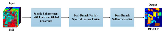
Figure 1.
Flowchart of the proposed dual-branch extraction and classification method (DBECM). HSI: hyperspectral images.
2.1. Sample Enhancement with Local and Global Constraint
A schematic diagram of the sample enhancement with local and global constraints is shown in Figure 2. In HSIs, training samples are represented as , where m represents the number of training samples. The label of the training sample is expressed as , and unlabeled samples are represented by , where n is the number of unlabeled samples.
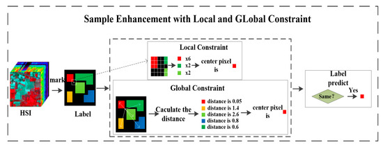
Figure 2.
Schematic diagram of the sample enhancement of local and global constraints.
For an unlabeled sample , represents a contiguous sample of a certain size around . represents the training sample nearby in the k-size space. is the intersection of and . If exists, the class label of the sample is calculated from the statistical distribution of . The class with the most training samples is defined as . If the number of such training samples is greater than (k−1)/2, the local constraint obtained by the unlabeled sample is premarked as . Conversely, if the above conditions are not met, the unlabeled sample is premarked as 0.
For global constraints, the image is a collection of samples of all categories that are further away from the unlabeled sample . The spectral angular distance (SAD) of each sample in and the unlabeled sample is calculated by Equation (1), among which the smallest one is selected as the premarking of the unlabeled sample . When all SAD values are greater than 1, the premark is defined as 0.
Only the unlabeled samples with the same nonzero labels by the local spatial constraints and the global spectral constraints are selected. The selected unlabeled samples are recorded as and , respectively, and the prelabels are determined by Equation (2):
Especially because the tracking algorithm of the prelabeled samples is the same, in the case of the same labeled samples, the training set and test set after completing the sample enhancement are fixed.
When the sample enhancement is completed, the number of samples is recalculated. The number of different class samples is balanced, which makes the training set more uniform and helps the network model to extract features.
2.2. Multiscale Spatial-Spectral Feature Fusion
HSIs are regarded as three-dimensional data cubes with both spatial and spectral information. In HSIs, the spectral characteristics of samples in the same class may vary due to the differences in imaging conditions, such as changes in illumination, environment, and atmosphere, as well as the change of time. In addition, limited by manufacturing techniques, the spatial resolution of hyperspectral remote sensing images is generally not high, so that the spatial features of ground targets are not fully extracted. Therefore, extracting complete and accurate joint spatial-spectral features is the key to improving the accuracy of HSIs classification.
The dual-branch spatial-spectral feature extraction and classification method is shown in Figure 3. In this method, a double-branch structure is constructed. The first branch is the LSTM unit that extracts the characteristics of the sequence signal. The specific structure of the LSTM unit is shown in Figure 4. For the full extraction of the spectral feature, the data of all spectral bands rather than dimensionality reduction data are taken as part of the input data in this branch. In order to extract the spatial information, the EMAP is applied to the HSIs data using PCA dimension reduction. The EMAP results are combined with the spectral data of the corresponding location to form the output vector. Since the combined spectral-EMAP data has no semantic order, a spatially spectral joint feature is extracted using a Bi-LSTM network, with 128 hidden nodes to ensure better feature extraction.
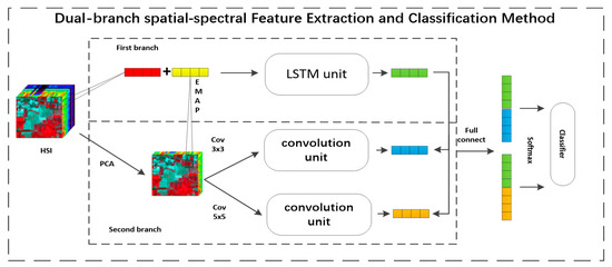
Figure 3.
Schematic diagram of dual-branch spatial-spectral feature extraction and classification method. PCA: principle component analysis. LSTM: long short-term memory. EMAP: expanded multi-attribute morphological profile. Cov: convolution.
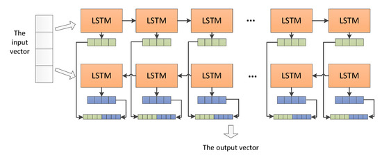
Figure 4.
Structure of the LSTM unit.
The LSTM is an improvement method on the standard recurrent neural network (RNN), and it is mainly improved in the addition of three door controllers: input gate, output gate, and forgetting gate. The structure of the three gate controllers is the same, which is mainly composed of a sigmoid function (σ) and a dot product operation (×). Since the value range of the sigmoid function is 0–1, the gate controller determines the proportion through which the information can pass by the value of sigmoid. Therefore, the weight control of the memory at different times is added, and a cross-layer connection is added to reduce the influence of the gradient disappearance problem. The LSTM is used to explore the dependence of the current state of the sequence information on the previous state. However, when nontime sequential vectors are involved, dependencies exist in both forward and backward directions. To solve this problem, a two-way LSTM [49] is proposed to exploit the forward and backward relationship of the sequential data. Therefore, the method proposed in this paper is also selected from the Bi-LSTM.
The EMAP is a set of multilevel features that perform a series of coarsening (closed operation) and refinement (opening) filtering on the image and can effectively describe the spatial information of the image.
The coarsening (closed operation) and the refinement (opening operation) are two important transformations for extracting the shape profile of the image. The open operation at x is defined as Equation (3):
where I is a binary image, x is a pixel on I, and X contains the connected domain of x.
By adding an attribute constraint to the open operation, the attribute open operation of the connected domain X is obtained by Equation (4):
where Τ(X) is an attribute of the connected domain X and λ is the attribute threshold. The attribute open transform of the entire binary image is defined by Equation (5):
In order to generalize the above transformation from the binary image to the grayscale image, each grayscale value of the grayscale image is sequentially used as a threshold value. The grayscale image is calculated by the threshold to obtain a series of binary images, which are recorded as Equation (6):
Then, the opening operation is taken for each binary image , and the maximum gray level in which the constraint is satisfied is taken as an output. The attribute of opening operation of the grayscale image I is obtained by Equation (7):
Similarly, the attribute of the closure operation of the grayscale image I is defined as Equation (8):
where is the attribute closure operation of the binary image.
According to different attribute thresholds for attribute opening and closing operations, the attribute opening profile and the attribute closing profile at the point x is obtained by Equation (9) for each pixel x on the image I.
In this paper, four kinds of attributes, including: the area length, the diagonal length of the circumscribed rectangle, the first-order invariant moment, and the standard deviation of the pixel values in the area, are selected.
The second structure is a 3D-CNN structure that extracts different spatial features by a two-scale convolution kernel. Using the dimensionality reduction method of the PCA, the input of the dual-scale architecture is the dimensionality reduction patch. In the two-scale architecture, convolution kernels consist of convolutional layers of 3 × 3 × 1 and 5 × 5 × 3, corresponding normalized layers and rectified linear unit (ReLU) active layers for extracting the spatial features, spectral features, and the correlation between space and spectrum in HSIs. Then the padding layer is also superimposed. Finally, the extracted features are flattened into a one-dimensional vector as the input of the next fully connected layer. The dual-scale convolution kernel in the DBECM shows excellent performance in local feature extraction.
As shown in Figure 5, all convolutional layer outputs of each convolution unit adopt a normalization strategy to improve the stability of the network in the convolution structure. Subsequent ReLU acts as a nonlinear activation function to activate the output of the convolution, which is expanded by a padding layer to its original size for convolution. To reduce overfitting, the dropout layer is adopted before outputting to the next convolution unit. The pooling layer is not used in the convolution unit, because the pooling operation improves the rotation invariance of the feature. However, in the hyperspectral remote sensing image classification task, the pooling operation greatly changes the spatial correlation of the target, so that the spatial information is no longer right.
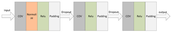
Figure 5.
Structure of the convolution unit. ReLU: rectified linear unit.
After the features are extracted in both structures, the extracted features are flattened into a one-dimensional vector. The features of the LSTM structure are respectively spliced with the features input full-connection layers of the two-scale CNN structures to form multiscale spatial-spectral joint features.
2.3. Dual-Branch Softmax Classifier
These features with different scales entered into two Softmax layers, respectively. The output of the Softmax layer represents the probability distribution of the classes derived from the different scale features. Considering the two outputs of the two Softmax layers, a new loss function is defined. In the test phase, the outputs of the two Softmax layers are used to predict the class label of the sample by multiple decision methods.
In the DBECM, Softmax is used for multiclass classification. The output of the Softmax function is used to represent the probability distribution of all classes, where the probability of each class is in the range of 0–1 and all the probabilities are added up to 1. Besides, considering the scales of convolution kernels used in this model are 3 × 3 × 1 and 5 × 5 × 3, which all have central structures, and in order to incorporate the center loss into the training process, a new loss function is proposed.
The loss function is determined by the cross-entropy of the real class and the output class probability, as well as the center loss. Since the network uses Softmax as the activation function, which has the characteristics of the block in the structure, the center loss is added as a part of the loss function in the network based on the prediction probability to improve the judgment of the features. The cross-entropy of the real class and output class probability is calculated as Equation (10):
where and are the probabilities that the i-th samples are assigned respectively to the c-th class according to the different scale features.
The center loss is defined as Equation (11):
where the learned feature corresponds to the i-th input spectra in the batch, and denotes the c-th class center defined by the averaging over the features in the z-th class.
The loss function is defined as Equation (12):
In the testing phase, the classification results are determined by the class probability distribution of these different scale features. The test sample {, ,…, } of the label {, ,…, } is predicted by Equation(13):
3. Results
Compared with several latest HSIs classification methods, two sets are selected as classical data to verify the performance of the proposed deep learning model in this section. In addition, parameters of the proposed network are discussed and analyzed.
3.1. Experimental Setup
In order to verify the classification performance of the proposed DBECM method, representative HSI classification methods based on the deep learning strategy, including DBN [50], CNN [49], PF-CNN [51], LSTM [52], 3D-CNN [46], and GLCM-CNN [53] are used for comparison. Additionally, the support vector machine (SVM) [33] is adopted. The classification performance of all these methods is measured by three common indicators: overall accuracy, average accuracy, and the Kappa coefficient.
The overall accuracy (OA) is defined as Equation (14):
where is the i-th correctly classified test sample and N is the total number of test samples.
The average accuracy (AA) is defined as Equation (15):
where M is the class number of each dataset, is the total test sample number of the i-th class, and is the j-th correctly classified test sample of class i.
All experimental results are obtained by the training set and the test set, which are randomly divided. In addition, all experimental results are the average of 10 independent running results. All experiments were performed by the Python language and TensorFlow + Keras. An Intel Core i7 CPU and a NVIDIA 1080Ti graphics card were used to implement the GPU computation.
For DBN, the radius of the search space neighborhood window is in the range of 3–21 with the interval of 2. For CNN, as shown in [51], the patch size for extracting spatial features is set to 5 × 5. For PF-CNN, the size of the adjacent pixel window is set to the same configuration as in [51]. For LSTM, we constructed a loop layer with 128 hidden nodes. For 3D-CNN, we set the window size of the 3D input to 27 × 27 as the settings in [46]. For GLCM-CNN, we set the window size to 27 × 27 as the settings in [53]. For the DBECM network proposed in this paper, the input spatial window size is 21 × 21. In the training process, the batch size of DBECM is 128, the optimization method used is as the stochastic gradient descent (SGD), the learning rate is 0.001, and the number of iterations is 1000.
In each dataset, 10% of each category is randomly selected from the labeled samples as a training set. More than twice of the training samples are selected as prelabeled samples from the unlabeled samples to expand the number of training samples through sample enhancement, and then the numbers of training samples in different classes are balanced. The remaining data is used for testing.
3.2. Classification Results
3.2.1. Indian Pines Dataset
Indian Pines: On 12 June 1992, the airborne visible/infrared imaging spectrometer sensor (AVIRIS) was acquired at the Indian pine test site in northwest Indiana, USA and consisted of 145 × 145 pixels and 220 spectral bands. The absorption bands 100–104, 150–163, and 220 were removed, and a total of 200 spectral bands were used. The spatial resolution of the dataset is 20 m per pixel, and the spectral resolution is 10 nm, which covers a range of 200 to 2400 nm. The pseudo-color composite image and its spectral curve are shown in Figure 6. Additionally, the number of training samples and test samples is shown in Table 1.
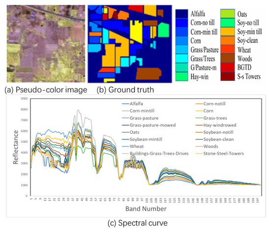
Figure 6.
Indian pines dataset. (a) is pseudo-color image of Indian pines dataset. (b) is its ground truth image. (c) is the spectral curve of Indian pines dataset.

Table 1.
Indian pines data for various training samples and test samples.
Table 2 records the average classification accuracy of the seven independent algorithms and their corresponding standard deviations. In Table 2, the first 16 rows correspond to the results of each class, and the last three rows are the results of the OA, AA, and Kappa for all classes. It can be seen from the table that the deep learning methods based on DBN, CNN, PF-CNN, 3D-CNN, and DBECM are superior to SVM due to their hierarchical nonlinear feature extraction capabilities. Only one-way LSTM with 128 nodes is worse than SVM. Compared with DBN and LSTM, since CNN and the other methods use multilayer convolution, the results of the feature extraction from HSIs data by the two-dimensional structure are better than DBN and LSTM, which only analyze the spectrum. Compared with CNN, PF-CNN has a better classification result due to the addition of available training samples. Compared with PF-CNN, 3D-CNN and GLCM-CNN combines spatial features and spectral features to improve the classification performance. Among the eight methods, the DBECM achieved the best classification results in most categories due to effective sample enhancement and the dual-branch spatial and spectral features fusion. In addition, DBECM improves at least 4.7%, 5.7%, and 5% in the OA, AA, and the Kappa, compared to other methods.
Table 2.
Classification results of seven methods of the Indian pines dataset in the 10% train set. OA: overall accuracy. AA: average accuracy. SVM: support vector machines. LSTM: long short-term memory. CNN: convolutional neural network. DBECM: dual-branch extraction and classification method.
Figure 7 shows the classification accuracy of each type of target under each method. It can be seen from the figure that the accuracy of the DBECM proposed in this paper is higher than that of several other methods, which proves that this method has a good classification performance. Figure 8 contains the true image of the Indian pines dataset and the classification results of the seven methods. The areas where the effect of the DBECM is greatly improved are marked with red frames. It can be seen that SVM, DBN, CNN, PF-CNN and LSTM misclassified many samples in the central region, especially in corn-notill, corn-mintill, soybean-notill, and soybean-mintill. To some extent, misclassification leads to scattering on the graph. Compared to these methods, the 3D-CNN and DBECM methods significantly improve the uniformity of the region, and, compared to 3D-CNN, the DBECM has a better classification accuracy in alfalfa, oats, and several classes of corn. Compared to the GLCM-CNN, which is also a dual-branch structure fused with spatial–spectral features, the DBECM still has advantages in OA, AA, and the Kappa, and the classification accuracy in multiple categories is close to 100%. This is because the DBECM increases the number of training set samples through prelabeling during the data enhancement phase and incorporates more spatial information into the network structure, not just texture features.
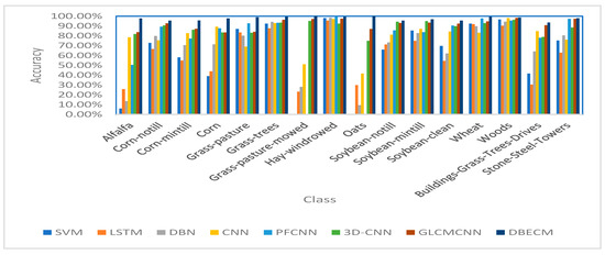
Figure 7.
Accuracy of different methods in the Indian pines dataset. SVM: support vector machine. CNN: convolutional neural network.
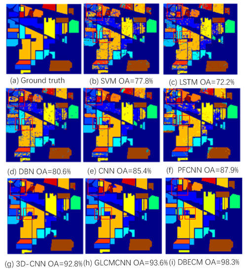
Figure 8.
The true value image of the Indian pines dataset and the classification results of the seven methods. (a) is a true value image, and (b–i) are the classification results of the SVM, LSTM, DBN, CNN, PF-CNN, 3D-CNN, GLCM-CNN, and DBECM. OA: overall average.
3.2.2. Pavia University Dataset
Pavia University: 8 July 2002, collected by the reflective optical system imaging spectrometer (ROSIS) while flying over Pavia in northern Italy. It consists of 610 × 340 pixels and 115 spectral bands. After removing 12 noise bands, 103 bands are used. The dataset has a spatial resolution of 1.3 m/pixel and a spectral range from 0.43–0.86 μm. The pseudo-color composite image and its spectral curve are shown in Figure 9.
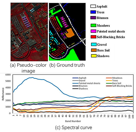
Figure 9.
Pavia University dataset. (a) is pseudo-color image of Pavia University dataset. (b) is its ground truth image. (c) is the spectral curve of Pavia University dataset.
In the dataset of Pavia University, each class randomly selects 10% of the samples for training.
Table 3 shows the number of training and test samples in the nine classes of the Pavia University image.
Table 3.
Pavia University data for various training samples and test samples.
The statistical classification results of the Pavia University dataset are shown in Table 4. As can be seen from the table that CNN, PF-CNN, 3D-CNN, and DBECM have better results than the SVM and DBN, the reason is that these methods extract spatial information through local connections and reduce network parameters through weight sharing. For the gravel class, the classification results for the SVM, DBN, and CNN are not satisfactory. Compared with these three algorithms, the DBECM improves 35.8%, 27.7%, and 11.8% in accuracy, respectively. For all categories, the DBECM classification accuracy is higher than 95%; especially, the classified accuracy of the painted metal sheets is 100%. Among the seven algorithms, the DBECM has the best results in the OA, AA, and Kappa indicators, with the improvement at least 3.9%, 7.5%, and 3.1% compared to other algorithms.
Table 4.
Classification results of the seven methods in the Pavia University dataset in the 10% train set.
Figure 10 shows the classification accuracy of each type of target under each method. It can be seen from the figure that the accuracy of the DBECM proposed in this paper is higher than that of several other methods, which proves that this method has a good classification effect. Figure 11 contains the true image of the Pavia University dataset and the classification results of the seven methods. The areas where the effect of the DBECM is greatly improved are marked with red frames. Due to similar spectral characteristics, many samples belonging to Bitumen are misclassified as asphalt. The proposed DBECM method can distinguish the two classes better. Compared with other methods, the DBECM has better classification performance and local accuracy in all categories. Compared to the GLCM-CNN, which is also a dual-branch structure fused with spatial–spectral features, the DBECM still has advantages in OA, AA, and the Kappa, and the classification accuracy in multiple categories is close to 100%. This is because the DBECM incorporates more spatial information into the network structure, not just texture features; besides, spectral curves of features with a classification accuracy rate close to 100% are quite different.
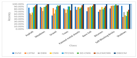
Figure 10.
Accuracy in different methods.
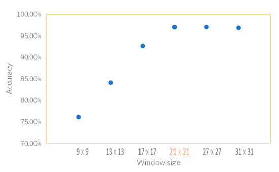
Figure 11.
Indian pines dataset OA with window size changes.
4. Discussion
In the DBECM, there are several important model parameters, including the window size, the selection of the training sets size, the parameters of the PCA process before the EMAP and the number of iterations.
4.1. Window Size
In order to find the optimal size of the input images, a univariate method is used to determine other factors. We select the size from the four candidate values of 13, 17, 21, and 27. Figure 11 shows the effect on the OA of different window sizes in the Indian pines dataset. As can be seen from the table, the OA increases with the expanding of the window size, and the size of 21 × 21 can achieve sufficiently high accuracy. After analyzing the trend in the figure, we conclude that the 21 × 21 can be selected as the optimal size, because it will take more time for calculations with the larger window size, as well as the improvement of accuracy is limited.
4.2. Training Set Size
The size of the training set can also have a significant impact on the result of the OA. Considering the difficulty of hyperspectral sample markers and the diversity of classes, the univariate method is also used to determine other factors. In this discussion, we select the training set sizes as 5%, 10%, 15%, and 20%. Figure 12 shows the relationship between the OA value of the Indian pine dataset and the training set selection ratio. Comparing the final OA values, we can know that the 10% selectivity can achieve the best accuracy. Increasing the training set size has a small boost of the accuracy and can cause limitations of the model. Therefore, the training set used in this paper is selected to be 10%. It can also be seen from the figure that the curve of the method proposed in this paper is above the image, indicating that this method is more suitable for the case of limited samples.
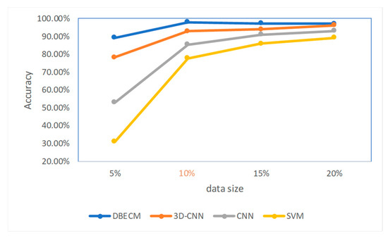
Figure 12.
Indian pines dataset OA changes with the training set selection ratio.
4.3. Parameter of PCA
Table 5 shows the OA values of the Indian pines dataset with and without PCA dimensionality reduction. Comparing the OA values of the two cases, it can be concluded that the use of a PCA dimensionality reduction is obviously helpful for the improvement of the OA value, because a PCA dimensionality reduction will retain most of the main information of the image and eliminate interference and it can improve the blurring of hyperspectral images due to poor imaging experiment.
Table 5.
The OA of Indian pines datasets in two different cases. PCA: principle component analysis.
The dimension after a PCA also has a certain impact on the performance of the classification. To investigate the impact of the dimension on the classification, the Indian pines dataset is used for verification. Figure 13 shows the OA values of the Indian pines dataset under the DBECM network in different dimensions. It can be seen from the figure that when the dimension after a PCA is 7, the OA value is the highest and the classification performance is the best.
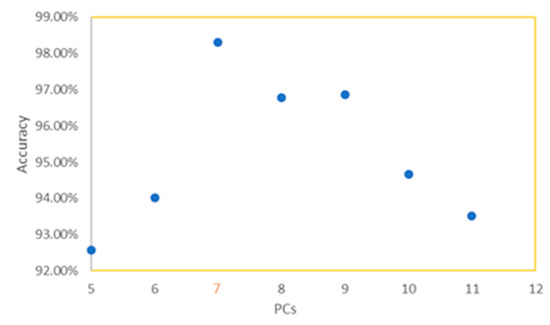
Figure 13.
Indian pines dataset OA changes with the training set selection ratio. PCs: principle components.
The relationship between a PCA dimension and the OA performance is further discussed in this section. When the dimensionality reduction dimensions are six, seven, and eight, the respective band patterns are shown in Figure 14. Table 6 shows the signal-to-noise ratio (SNR) of each PCs and the first principal component. Comparing the data in the table, the SNR is greater than 0 from the PCs8. Analyzing the features of Figure 14, when the dimension is seven, the seventh image still has some spatial detail information that does not exist in the other images. When the dimension is a reduction of eight, there are many obvious noises on the eighth image, which will interfere with the extraction of the EMAP. When the dimensionality reduction dimension is bigger than eight, the backward bands are meaningless noise images, which have a weakening effect on image feature extraction. Therefore, when the dimension reduced by a PCA is seven, the best result is achieved.
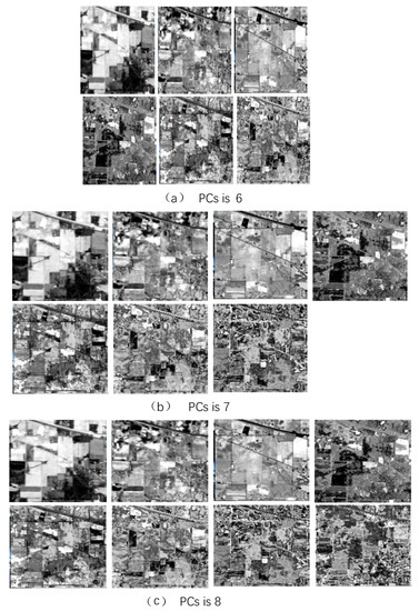
Figure 14.
The Indian pines dataset shows the different band diagrams for different dimensionality dimensions. (a) for the 6-dimensional result graph, (b) for the 7-dimensional result graph, and (c) for the 8-dimensional result graph.
Table 6.
The signal-to-noise ratio (SNR) of every principle components (PCs) with PCs1.
4.4. Network Runtime Analysis
Table 7 lists the training time and testing time for the seven algorithms on the Indian pines. As shown in the table, the LSTM and DBN are faster in training time than the PF-CNN, CNN, 3D-CNN, and DBECM, because the input of these two methods is a one-dimensional vector. The PF-CNN and 3D-CNN are time-consuming methods among all the comparison methods, since the three-dimensional convolution operation leads to an increase in the network parameters, while the 3D-CNN requires more time. The PF-CNN takes more time due to the expansion of a large number of training samples. The time of the DBECM is longer than the 3D-CNN and PF-CNN in training. Since under the same sample size, the DBECM uses both 3D convolution and the feature extraction for 1D vectors. The amount of data processing is even larger, so it takes more time.
Table 7.
Seven algorithms under the Indian pines dataset schedule.
4.5. Number of Iterations
To determine the optimal number of iterations, a loss curve is generated in real-time during the training process. Figure 15 is the loss curve. We can know that, when the number of iterations is 1000, a lower loss can be reached, which is 0.35. When the number of iterations increases, the loss does not decrease significantly, so the number of iterations is determined to be 1000.
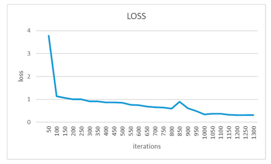
Figure 15.
Loss curve.
5. Conclusions
In this paper, a method named the DBECM is proposed for hyperspectral images classification under limited training samples. Specifically, a sample enhancement process based on global and local constraints is proposed. Unlabeled samples can be premarked to increase the sample size using local and global constraints based on a small number of samples that have been marked. The combination of two constraints guarantees the accuracy of premarking. Besides that, the sample enhancement process balances the number of samples for reducing overfitting. A two-branch spatial-spectral feature extraction and classification structure is established. Two different neural networks are used to realize the simultaneous extraction and fusion of two-way spatial-spectral features for increasing the completeness and accuracy of the features. The loss function and classifier based on a two-way prediction probability are designed to improve the classification accuracy. Last, the experiments are conducted in two typical, public datasets. The results show that this method is better than the SVM, CNN, and other traditional methods. Especially, in some classes, the correct rate is 100%. Compared with other methods, this method significantly improves the detailed information of the edge of the object while maintaining a high classification accuracy and improving the classification accuracy of the easy-mixing class.
However, there are some shortcomings in the DBECM network. The major one is that the time of the DBECM network training is longer than other methods. To overcome these shortcomings, we will introduce more sophisticating optimization techniques in our future works.
Author Contributions
B.N. and J.L. contributed equally to the study and are co-first authors. B.N. conceived and designed the algorithms and wrote the paper; J.L. analyzed the data, contributed data collection, reviewed the paper and organized the revision. Y.S. and H.Z. performed the experiments. All authors have read and agreed to the published version of the manuscript.
Funding
This research was funded by the Major Special Project of the China High-Resolution Earth Observation System, the funding 41416040203, the funding FRF-GF-18-008A and the funding FRF-BD-19-002A.
Acknowledgments
We would like to thank the editor and reviewers for their reviews that improved the content of this paper.
Conflicts of Interest
The authors declare no conflict of interest.
References
- Green, R.O.; Eastwood, M.L.; Sarture, C.M.; Chrien, T.G.; Aronsson, M.; Chippendale, B.J.; Faust, J.A.; Pavri, B.E.; Chovit, C.J.; Solis, M.; et al. Imaging spectroscopy and the Airborne Visible/Infrared Imaging Spectrometer (AVIRIS). Remote Sens. Environ. 1998, 65, 227–248. [Google Scholar] [CrossRef]
- Pearlman, J.; Carman, S.; Segal, C.; Jarecke, P.; Clancy, P.; Browne, W. Overview of the Hyperion Imaging Spectrometer for the NASA EO-1 mission. In Proceedings of the IEEE 2001 International Geoscience and Remote Sensing Symposium (Cat. No.01CH37217), Sydney, Australia, 9–13 July 2001; pp. 3036–3038. [Google Scholar]
- Pearlman, J.S.; Barry, P.S.; Segal, C.C.; Shepanski, J.; Beiso, D.; Carman, S.L. Hyperion, a space-based imaging spectrometer. IEEE Trans. Geosci. Remote Sens. 2003, 41, 1160–1173. [Google Scholar] [CrossRef]
- Ghamisi, P.; Mura, M.D.; Benediktsson, J.A. A Survey on Spectral–Spatial Classification Techniques Based on Attribute Profiles. IEEE Trans. Geosci. Remote Sens. 2015, 53, 2335–2353. [Google Scholar] [CrossRef]
- Li, J.; Khodadadzadeh, M.; Plaza, A.; Jia, X.; Bioucas-Dias, J.M. A discontinuity preserving relaxation scheme for spectral–spatial hyperspectral image classification. IEEE J. Sel. Top. Appl. Earth Obs. Remote Sens. 2016, 9, 625–639. [Google Scholar] [CrossRef]
- Gu, Y.; Liu, T.; Jia, X.; Benediktsson, J.A.; Chanussot, J. Nonlinear multiple kernel learning with multiple-structure-element extended morphological profiles for hyperspectral image classification. IEEE Trans. Geosci. Remote Sens. 2016, 54, 3235–3247. [Google Scholar] [CrossRef]
- Meola, J.; Eismann, M.T.; Moses, R.L.; Ash, J.N. Application of model-based change detection to airborne VNIR/SWIR hyperspectral imagery. IEEE Trans. Geosci. Remote Sens. 2012, 50, 3693–3706. [Google Scholar] [CrossRef]
- Demir, B.; Bovolo, F.; Bruzzone, L. Updating land-cover maps by classification of image time series: A novel change-detection-driven transfer learning approach. IEEE Trans. Geosci. Remote Sens. 2013, 51, 300–312. [Google Scholar] [CrossRef]
- Wu, C.; Du, B.; Zhang, L. Slow feature analysis for change detection in multispectral imagery. IEEE Trans. Geosci. Remote Sens. 2014, 52, 2858–2874. [Google Scholar] [CrossRef]
- Hu, F.; Xia, G.; Hu, J.; Zhang, L. Transferring deep convolutional neural networks for the scene classification of high-resolution remote sensing imagery. Remote Sens. 2015, 7, 14680–14707. [Google Scholar] [CrossRef]
- Li, X.; Mou, L.; Lu, X. Scene parsing from an MAP perspective. IEEE Trans. Cybern. 2015, 45, 1876–1886. [Google Scholar]
- Olmanson, L.G.; Brezonik, P.L.; Bauer, M.E. Airborne hyperspectral remote sensing to assess spatial distribution of water quality characteristics in large rivers: The Mississippi River and its tributaries in Minnesota. Remote Sens. Environ. 2013, 130, 254–265. [Google Scholar] [CrossRef]
- Moran, M.S.; Inoue, Y.; Barnes, E.M. Opportunities and limitations for image-based remote sensing in precision crop management. Remote Sens. Environ. 1997, 61, 319–346. [Google Scholar] [CrossRef]
- Lan, J.H.; Zou, J.L.; Hao, Y.S.; Zeng, Y.L.; Zhang, Y.Z.; Dong, M.W. Research progress on unmixing of hyperspectral remote sensing imagery. J. Remote Sens. 2018, 22, 13–27. [Google Scholar]
- Shao, Y.; Lan, J.; Zhang, Y.; Zou, J. Spectral Unmixing of Hyperspectral Remote Sensing Imagery via Preserving the Intrinsic Structure Invariant. Sensors 2018, 18, 3528–3552. [Google Scholar] [CrossRef]
- Zou, J.; Lan, J.; Shao, Y. A hierarchical sparsity unmixing method to address endmember variability in hyperspectral image. Remote Sens. 2018, 10, 738–760. [Google Scholar] [CrossRef]
- Zou, J.; Lan, J. A Multiscale Hierarchical Model for Sparse Hyperspectral Unmixing. Remote Sens. 2019, 11, 500–515. [Google Scholar] [CrossRef]
- Shao, Y.; Lan, J. A Spectral Unmixing Method by Maximum Margin Criterion and Derivative Weights to Address Spectral Variability in Hyperspectral Imagery. Remote Sens. 2019, 11, 1045–1073. [Google Scholar] [CrossRef]
- Yu, L.; Lan, J.; Zeng, Y.; Zou, J.; Niu, B. One hyperspectral object detection algorithm for solving spectral variability problems of the same object in different conditions. Appl. Rem. Sens. 2019, 13, 026514. [Google Scholar] [CrossRef]
- Hang, R.; Liu, Q.; Song, H.; Sun, Y. Matrix-Based Discriminant Subspace Ensemble for Hyperspectral Image Spatial-Spectral Feature Fusion. IEEE Trans. Geosci. Remote Sens. 2016, 54, 783–794. [Google Scholar] [CrossRef]
- Hughes, G. On the Mean Accuracy of Statistical Pattern Recognizers. IEEE Trans. Inf. Theory 1968, 14, 55–63. [Google Scholar] [CrossRef]
- Zhang, L.; Zhang, L.; Tao, D.; Huang, X. On Combining Multiple Features for Hyperspectral Remote Sensing Image Classification. IEEE Trans. Geosci. Remote Sens. 2012, 50, 879–893. [Google Scholar] [CrossRef]
- Xu, J.; Hang, R.; Liu, Q. Patch-Based Active Learning PTAL for Spectral-Spatial Classification on Hyperspectral Data. Int. J. Remote Sens. 2014, 35, 1846–1875. [Google Scholar] [CrossRef]
- Palsson, F.; Sveinsson, J.R.; Ulfarsson, M.O.; Benediktsson, J.A. Model-Based Fusion of Multi- and Hyperspectral Images Using PCA and Wavelets. IEEE Trans. Geosci. Remote Sens. 2015, 53, 2652–2663. [Google Scholar] [CrossRef]
- Kuo, B.; Landgrebe, D.A. Nonparametric Weighted Feature Extraction for Classification. IEEE Trans. Geosci. Remote Sens. 2004, 42, 1096–1105. [Google Scholar]
- Chen, H.T.; Chang, H.W.; Liu, T.L. Local Discriminant Embedding and Its Variants. In Proceedings of the IEEE Computer Society Conference on Computer Vision and Pattern Recognition (CVPR’05), San Diego, CA, USA, 20–25 June 2005; Volume 2, pp. 846–853. [Google Scholar]
- Wang, Q.; Meng, Z.; Li, X. Locality Adaptive Discriminant Analysis for Spectral–Spatial Classification of Hyperspectral Images. IEEE Geosci. Remote Sens. Lett. 2017, 14, 2077–2081. [Google Scholar] [CrossRef]
- Reed, I.S.; Yu, X. Adaptive multiple-band CFAR detection of an optical pattern with unknown spectral distribution. IEEE Trans. Acoust. Speech Signal Process. 1990, 38, 1760–1770. [Google Scholar] [CrossRef]
- Villa, A.; Benediktsson, J.A.; Chanussot, J.; Jutten, C. Hyperspectral Image Classification with Independent Component Discriminant Analysis. IEEE Trans. Geosci. Remote Sens. 2011, 49, 4865–4876. [Google Scholar] [CrossRef]
- Goel, P.; Prasher, S.; Patel, R.; Landry, J.; Bonnell, R.; Viau, A. Classification of hyperspectral data by decision trees and artificial neural networks to identify weed stress and nitrogen status of corn. Comput. Electron. Agric. 2003, 39, 67–93. [Google Scholar] [CrossRef]
- Ham, J.; Chen, Y.; Crawford, M.M.; Ghosh, J. Investigation of the random forest framework for classification of hyperspectral data. IEEE Trans. Geosci. Remote Sens. 2005, 43, 492–501. [Google Scholar] [CrossRef]
- Joelsson, S.R.; Benediktsson, J.A.; Sveinsson, J.R. Random forest classifiers for hyperspectral data. In Proceedings of the IEEE International Geoscience and Remote Sensing Symposium, 2005. IGARSS ‘05, Seoul, Korea, 29 July 2005; Volume 1, p. 4. [Google Scholar]
- Melgani, F.; Bruzzone, L. Classification of hyperspectral remote sensing images with support vector machines. IEEE Trans. Geosci. Remote Sens. 2004, 42, 1778–1790. [Google Scholar] [CrossRef]
- Benediktsson, J.A.; Palmason, J.A.; Sveinsson, J.R. Classification of hyperspectral data from urban areas based on extended morphological profiles. IEEE Trans. Geosci. Remote Sens. 2005, 43, 480–491. [Google Scholar] [CrossRef]
- Fauvel, M.; Benediktsson, J.A.; Chanussot, J.; Sveinsson, J.R. Spectral and spatial classification of hyperspectral data using SVMs and morphological profiles. IEEE Trans. Geosci. Remote Sens. 2008, 46, 3804–3814. [Google Scholar] [CrossRef]
- Li, J.; Marpu, P.R.; Plaza, A.; Bioucas-Dias, J.M.; Benediktsson, J.A. Generalized composite kernel framework for hyperspectral image classification. IEEE Trans. Geosci. Remote Sens. 2013, 51, 4816–4829. [Google Scholar] [CrossRef]
- Qian, Y.; Ye, M.; Zhou, J. Hyperspectral image classification based on structured sparse logistic regression and three-dimensional wavelet texture features. IEEE Trans. Geosci. Remote Sens. 2013, 51, 2276–2291. [Google Scholar] [CrossRef]
- Jia, S.; Shen, L.; Li, Q. Gabor feature-based collaborative representation for hyperspectral imagery classification. IEEE Trans. Geosci. Remote Sens. 2015, 53, 1118–1129. [Google Scholar]
- LeCun, Y.; Bengio, Y.; Hinton, G. Deep learning. Nature 2015, 521, 436–444. [Google Scholar] [CrossRef]
- Hinton, G.E.; Salakhutdinov, R.R. Reducing the dimensionality of data with neural networks. Science 2006, 313, 504–507. [Google Scholar] [CrossRef]
- Vincent, P.; Larochelle, H.; Lajoie, I.; Bengio, Y.; Manzagol, P.-A. Stacked denoising autoencoders: Learning useful representations in a deep network with a local denoising criterion. J. Mach. Learn. Res. 2010, 11, 3371–3408. [Google Scholar]
- Krizhevsky, A.; Sutskever, I.; Hinton, G.E. ImageNet classification with deep convolutional neural networks. Adv. Neural Inf. Proc. Syst. 2012, 25, 1097–1105. [Google Scholar] [CrossRef]
- Zhao, W.; Du, S. Spectral spatial feature extraction for hyperspectral image classification: A dimension reduction and deep learning approach. IEEE Trans. Geosci. Remote Sens. 2016, 54, 4544–4554. [Google Scholar] [CrossRef]
- Zhao, W.; Du, S. Learning multiscale and deep representations for classifying remotely sensed imagery. ISPRS J. Photogramm. Remote Sens. 2016, 113, 155–165. [Google Scholar] [CrossRef]
- Chen, Y.; Jiang, H.; Li, C.; Jia, X.; Ghamisi, P. Deep Feature Extraction and Classification of Hyperspectral Images Based on Convolutional Neural Networks. IEEE Trans. Geosci. Remote Sens. 2016, 54, 6232–6251. [Google Scholar] [CrossRef]
- Liu, Q.; Zhou, F.; Hang, R.; Yuan, X. Bidirectional-Convolutional LSTM Based Spectral-Spatial Feature Learning for Hyperspectral Image Classification. Remote Sensing. 2017, 9, 1330–1347. [Google Scholar]
- Paoletti, M.E.; Haut, J.M.; Plaza, J.; Plaza, A. A new deep convolutional neural network for fast hyperspectral image classification. ISPRS J. Photogram. Remote Sens. 2017, 145, 120–147. [Google Scholar]
- Schuster, M.; Paliwal, K.K. Bidirectional recurrent neural networks. IEEE Trans. Signal Process. 1997, 45, 2673–2681. [Google Scholar] [CrossRef]
- Hu, W.; Huang, Y.; Wei, L.; Zhang, F.; Li, H. Deep convolutional neural networks for hyperspectral image classification. J. Sens. 2015, 2015, 258619. [Google Scholar] [CrossRef]
- Chen, Y.; Zhao, X.; Jia, X. Spectral–spatial classification of hyperspectral data based on deep belief network. IEEE J. Sel. Topics Appl. Earth Observ. Remote Sens. 2015, 8, 2381–2392. [Google Scholar] [CrossRef]
- Li, W.; Wu, G.D.; Zhang, F. Hyperspectral image classification using deep pixel-pair features. IEEE Trans. Geosci. Remote Sens. 2016, 55, 844–853. [Google Scholar] [CrossRef]
- Mou, L.; Ghamisi, P.; Zhu, X.X. Deep recurrent neural networks for hyperspectral image classification. IEEE Trans. Geosci. Remote Sens. 2017, 55, 3639–3655. [Google Scholar] [CrossRef]
- Zhao, W.; Li, S.; Li, A.; Zhang, B.; Li, Y. Hyperspectral images classification with convolutional neural network and textural feature using limited training samples. Remote Sens. Lett. 2019, 10, 449–458. [Google Scholar] [CrossRef]


© 2020 by the authors. Licensee MDPI, Basel, Switzerland. This article is an open access article distributed under the terms and conditions of the Creative Commons Attribution (CC BY) license (http://creativecommons.org/licenses/by/4.0/).