Preliminary Evaluation of the Error Budgets in the TALIS Measurements and Their Impact on the Retrievals


1
Key Laboratory of Microwave Remote Sensing, National Space Science Center, Chinese Academy of Sciences, Beijing 100190, China
2
University of Chinese Academy of Sciences, Beijing 100094, China
*
Author to whom correspondence should be addressed.
Remote Sens. 2020, 12(3), 468; https://doi.org/10.3390/rs12030468
Submission received: 10 December 2019
/
Revised: 27 January 2020
/
Accepted: 29 January 2020
/
Published: 2 February 2020
(This article belongs to the Special Issue Remote Sensing of Atmospheric Components and Water Vapor)
Abstract
:The THz Atmospheric Limb Sounder (TALIS) is a Chinese sub-millimeter limb sounder being designed by National Space Science Center of the Chinese Academy of Sciences to measure the temperature and chemical constituents vertically in the middle and upper atmosphere, with good precision and vertical resolution. This paper presents a simulation study that assesses the measurement errors and their impacts on the retrievals. Three error sources, including instrument uncertainties, calibration errors and a priori errors, are considered. The sideband weight uncertainty, the local oscillator, the pointing angle offsets and the measurement noise (NEDT), are considered as instrument uncertainties. Calibration errors consist of the hot target offset, the nonlinearity residual of the two-point calibration, use of the Rayleigh–Jeans (R–J) approximation and the choice of the antenna pattern. A priori profile errors of temperature, pressure and species are also considered. The results suggest that the antenna pattern mainly affects the retrievals in the troposphere. The NEDT is a major error source affecting all of the retrievals. The R–J approximation has a great impact upon the retrievals at 643 GHz, and should not be used. The local oscillator offset leads to an obvious error above 50 km. The effect of nonlinearity residuals cannot be neglected above 70 km. The impact of the sideband weight uncertainty and the hot target offset are relatively small. The pointing and the a priori errors can be neglected in most observation regions.
1. Introduction
Observation of the long-term evolution of the chemical species and the status of Earth’s atmosphere is essential for scientists to understand the physical and chemical processes in the atmosphere and to assess the changes of climate. A satellite is the only platform which can provide the daily global coverage of this information. Generally, three ways of observation can be used to monitor atmosphere: nadir observation, occultation observation and limb observation. Limb sounding is more appropriate for atmospheric species detection, since it has good vertical resolution and wide altitude range [1]. Several frequency regions have been adopted to monitor the changes in the atmosphere, ranging from ultraviolet to terahertz. Among others, the terahertz frequency region has the advantage of being independent of the day–night cycle.
There are already many infrared limb sounders, such as MIPAS and SCIAMACHY on the Envisat satellite, and occultation instruments such as SAGE, SciSat-FTS and GOMOS used for middle and upper atmosphere detection.
Terahertz limb sounding techniques have been used for deriving the information of Earth’s atmosphere for more than twenty years. The first Microwave Limb Sounder (MLS) onboard the Upper Atmosphere Research Satellite (UARS) launched in 1991 provided atmospheric data of temperature and species such as ClO, O3, H2O, SO2, CH3CN and HNO3 [2,3,4]. This information helps scientists understand the physical and chemical processes which lead to the O3 depletion. The Sub-Millimeter Radiometer (SMR) carried by the Odin satellite observed the atmospheric limb for half of the observation time, producing various species profiles in the middle atmosphere such as O3, ClO, N2O, HNO3, H2O, CO and NO, as well as isotopes of H2O, O3 and ice clouds with a high vertical resolution of 1–2 km [5,6,7,8]. MLS onboard the Aura satellite has heritage from the UARS-MLS experiment, and it is improved to measure more species with better global and temporal coverage, better spatial resolution and better precision [9,10,11,12,13]. Its major productions include OH, HO2, H2O, O3, HCl, ClO, HOCl, BrO, HNO3, N2O, CO, HCN, CH3CN, SO2 and the ice cloud [14]. The Superconducting Submillimeter-wave Limb–Emission Sounder (SMILES) onboard the Japanese Experiment Module (JEM) of the International Space Station (ISS) successfully demonstrated the performance of 4K-cooled Superconductor–Insulator–Superconductor (SIS) mixers, and gave observations of various chemical species [15,16,17,18,19,20].
Since Aura-MLS and Odin-SMR have worked for more than ten years, and the observation may be stopped in a few years, the follow-on instruments are imperatively needed to fill the gap. Currently, Stratospheric Inferred Winds (SIW) and SMILES-2 are being developed in Sweden and Japan, respectively [21,22,23]. SIW can measure horizontal wind vectors within 30–90 km, and provide the profiles of temperature, O3, H2O and other species. SMILES-2 is designed to measure the horizontal wind vectors, temperature and molecules at the range of 15−180 km.
The THz Atmospheric Limb Sounder (TALIS) is the first Chinese microwave limb sounder being developed in the National Space Science Center, the Chinese Academy of Sciences (NSSC, CAS). It is designed to measure atmospheric temperature, pressure and various chemical species, from 10 to 100 km with good precision and resolution. TALIS has four microwave radiometers covering 118, 190, 240 and 643 GHz. Fast Fourier Transform (FFT) spectrometers of 2 GHz bandwidth with 2 MHz resolution are used to improve the measurement performance. The observation performance of TALIS has been estimated in our previous study [24]. In this study, the impacts of the instrument uncertainties, calibration errors and a priori errors on the retrieval are estimated.
2. Description of TALIS
The THz Atmospheric Limb Sounder (TALIS) payload and observation characteristics are summarized in Table 1. The satellite for TALIS is designed at an orbit of 600 km. TALIS will use four heterodyne microwave radiometers that operate at four frequency regions about 118 GHz, 190 GHz, 240 GHz and 643 GHz to scan the atmospheric limb from about 0 to 100 km. The 1.6 m offset parabolic antenna provides the field of view (FOV) at the tangent point of about 5.5 km, 3.8 km, 3.3 km and 0.96 km, respectively. Two calibration targets (a hot target and an extra target) are set at the end of the arm. The hot target is used for the radiometer two-point calibration. The extra target is used to estimate the antenna effect and the nonlinearity. TALIS will view the hot target and the extra target at first for 3 s, and then scan the limb from 0 to 100 km in 10 s. Finally, it will view the cold space (used as a cold target) at 200 km for 5 s. The process of retrace (from 200 km to the surface) is the same (also record data). Four heterodyne radiometers operate in double-sideband mode (DSB). Eleven FFT spectrometers of 2 GHz bandwidth with 2 MHz resolution will be used to improve the performance of the observation. The spectral bands of TALIS are summarized in Table 2. The 118 GHz is used for temperature, 190 GHz for H2O, 240 GHz for O3, 643 GHz for HCl and other trade gases retrievals. More details are provided in [24].
3. Error Characterization and Simulation Method
3.1. Errors Description
3.1.1. Instrument Uncertainties
Instrument uncertainties come from the instrument itself, and usually cannot be corrected completely. The impacts of instrument uncertainties which cannot be corrected have to be assessed in order to quantify the accuracy of such a retrieval [25].
In a radiometer, the heterodyne mixer will convert the signal which is coming from the antenna to the intermediate frequency. Double sideband (DSB) and single sideband (SSB) are two modes of receivers commonly used in the radiometer. The SSB mode can keep the complete spectral lines, while the DSB mode can cover more spectral lines, since the upper and lower sideband signals will be folded together. In addition, the system temperature of the DSB receiver is lower than that of the SSB receiver. However, a sideband weight inconsistency commonly exists in the double-sideband radiometer. The theoretical value of the output radiance of a DSB receiver can be described as [26]:
where represents the channel, represents the measurement frequency, is the intermediate frequency, is the radiance after the mixer, is the radiance after the antenna, and are the lower and upper sideband response, respectively. In an ideal DSB radiometer, the sideband response of the lower and upper sideband should be consistent (0.5). In this simulation, an uncertainty of 0.2% is assumed in order to evaluate the retrieval error induced by the sideband weight. The assumed uncertainty of this sideband weight comes from our radiometer test.
The stability of local oscillator frequency is very important, since it controls which line will be detected. Although it is a systematic error that can be corrected before launch, the local oscillator frequency will vary over the time in which one year goes by. A 0.5 MHz offset which may have occurred after several years is assumed to estimate the effect. This value of uncertainty is assumed according to the work by Baron et al. (2018) [21].
The geometrical tangent height is a key parameter, and is usually obtained from the satellite navigation system. However, the star tracker data is sometimes not very accurate, and the pointing angle (Line of sight, LOS) error should be considered. Fortunately, pointing can be retrieved along with temperature and species in a retrieval method. To estimate the effect, a 0.021° (~1 km) offset is added to the simulation, and it will be retrieved simultaneously with the products. The uncertainty of the pointing offset is assumed according to the work of Baron et al. (2011) [17].
Measurement noise, that is noise equivalent differential temperature (NEDT) is the most important error that worsens the precision of retrievals. It is a statistical uncertainty that cannot be calibrated. The standard deviation (STD) can be calculated from the radiometric sensitivity equation:
where is the system noise temperature, which is the sum of the receiver temperature and the atmospheric temperature received by the antenna, is the noise equivalent spectral resolution, and is the integration time for measuring a single spectrum.
The assumed instrument uncertainties are summarized in Table 3.
3.1.2. Calibration Errors
Calibration is important, since it can produce the calibrated limb radiances. These errors in calibration should be avoided in some degree. However, residual errors will also remain after data processing.
The two-point calibration is a widely used method for microwave radiometer calibration [27,28]. The schematic of two-point calibration is illustrated in Figure 1.
The two-point calibration equation can be established as [29]:
where represents the channel, , , are the counts of Earth, hot and cold targets, respectively. , are the radiance of the hot target and the cold space obtained by the instrument, respectively. means the system nonlinearity difference, is the nonlinearity coefficient. The possible error sources from calibration are the residual nonlinearity radiance of calibration and the hot target offset, due to the instability of the calibration target. In this study, the hot target temperature is added by a −0.5 K offset to produce the uncertainty in calibration. The residual nonlinearity brightness temperature is set to a standard deviation of 0.3 K, which is a typical value measured by the radiometer test. Another possible source of error is the Rayleigh–Jeans (R–J) approximation used in radiometric calibration [30]. R–J approximation can convert radiance to brightness temperature by using a linear equation, and is widely used in radiometric calibration at the MMW band up to the THz band. However, R–J approximation will lead to a brightness temperature error which varies with frequency and temperature, and it is not easily corrected by adding an offset. In this simulation, in Equation (3) is replaced by when using the R–J approximation, and and are set to 2.73 K and 300 K, respectively. The variations of calibration errors with temperature and count ratio are shown in Figure 2. The count ratio means . Figure 2 shows that although the differences seem to be a constant error above 50 K, it also varies with count ratio. So, it cannot be corrected easily.
TALIS measures atmospheric limb radiances captured by the antenna. The radiance which is accepted by the antenna can be expressed by:
where represents the channel, represents the antenna received radiance, represents the radiance emitted from the atmosphere, describes the normalized antenna response function, describes the frequency response of the radiometer, and is the solid angle. The integrals are estimated over the full range of frequencies and solid angles where instrument response exists.
Using the Planck function to convert the radiance to brightness temperature, the antenna temperature can be described [31,32,33]:
where represents the antenna temperature, represents the earth scene component of the antenna temperature, represents the spillover emission, represents the coefficient of spillover correction. In addition, is the atmospheric emission brightness temperature, is the main beam efficiency and is the sidelobe contribution.
Antenna pattern plays an important role in atmospheric limb sounding, since the atmospheric profiles varies rapidly in some regions. The antenna patterns of TALIS are shown in Figure 3, and the fields of view (FOVs) are 5.5 km, 3.8 km, 3.3 km and 0.96 km, respectively. Usually, a 3 dB beamwidth (full width between half-power points) of the antenna pattern is considered as the main beam. However, the sidelobe contribution is not easily estimated, and this has a large impact on the measured radiance, especially in the limb sounding. Thus, how the antenna pattern affects the retrievals should be evaluated. In this simulation study, 2.5 times the main beamwidth of the antenna patterns is used to calculate the measured radiances, since it is usually used to represent the whole antenna pattern in calculation. The antenna patterns of the main beamwidth are used in retrieval in order to estimate the retrieval errors that may be induced by the antenna.
The assumed errors are summarized in Table 4.
3.1.3. A Priori Errors
The external errors mainly come from the forward model and the a priori profiles of temperature, species and pressure. The model error could not be estimated, since there is no absolute value that can be measured. So, no forward model errors are applied in this study.
The trace gas species can be retrieved by using the optimal estimation (OEM) retrieval method, which requires good knowledge of the atmospheric profiles as well as the measurement noise [34]. Since the method involves the nonlinear weighted least squares optimization and includes the use of a priori constraints for regularization, the a priori data mainly affects the region where measurement information is lacking, and the noise dominates the region where the measurement signal is large [35].
To estimate the effect of the a priori profile, the species profiles are multiplied by 120%, which is to serve as the a priori profiles, and the temperature profile is added as a 5 K offset. They are the standard deviation commonly used in building the a priori covariance matrix [36]. Pressure can be retrieved together with temperature, and a 5% error is added to the pressure profile to be the a priori pressure profile.
The assumed uncertainties are summarized in Table 5.
3.2. Model and Retrieval Method
In order to retrieve the atmospheric information, an accurate forward model which can simulate the radiative transfer, spectroscopy and instrumental characteristics, are necessary. In limb sounding, scattering can usually be neglected above the upper troposphere, since there are almost no clouds at these altitudes. While polar stratospheric clouds can be present, the particle sizes are smaller than the TALIS observation wavelengths.
The cloud-free radiative transfer equation can be described as:
where is the radiance, is the absorption coefficient, and means the two position of the radiance, and is the opacity or optical thickness. represents the atmospheric emission which is given by the Planck function.
The optimal estimation method (OEM) is the most widely used retrieval method in atmospheric sounding [34]. The cost function in the retrieval method can be defined as:
where is a priori state vector, and are the covariance matrices representing the variability of the state vector and the measurement error vector, respectively. The core theory of OEM is to compare the simulated radiance with the observed radiance until the state which minimizes the could be found.
The Levenberg–Marquardt method, which is the modification of the Gauss–Newton iterative, is used to solve the nonlinear problem [37]. The solution is given by:
where denotes the Levenberg–Marquardt parameter, and represents the weighting function matrix (Jacobian).
The error estimates induced by random and systematic uncertainties are given by:
where is the error induced by perturbing the parameters and is the state vector retrieved after changing the parameter according to its uncertainty, while is the state vector retrieved before changing the parameter.
In the following simulations, the Atmospheric Radiative Transfer Simulator (ARTS) is used to calculate the measured radiance [38]. The retrieval tool is Qpack, which is the OEM tool developed for interaction with ARTS [39]. Temperature, H2O, O3 and HCl are treated as main products of the 118 GHz, 190 GHz, 240 GHz and 643 GHz radiometers, respectively. A mid-latitude summer atmospheric condition extracted from FASCOD, which is provided by ARTS, is chosen to perform the simulation, and local spherical homogeneity is assumed. A vertical retrieval grid of 2.5 km resolution is selected. The choice of a retrieval grid is closely related to the antenna field of view (FOV). Generally speaking, the resolution of the retrieval grid should match the antenna FOV. Degrading the vertical resolution can improve the retrieval precision and increase the retrieval speed. The retrieval precision of the four radiometers with different retrieval grids are shown in Figure 4. There is usually a trade-off between precision and resolution according to different applications.
4. Results
4.1. 118 GHz
The temperature retrieval errors induced by instrument uncertainties are shown in Figure 5. The error induced by local oscillator offset (LO) is around 5 K above 60 km, since the line width is quite narrow in the upper atmosphere. Sideband weight causes an error of 1 K in the stratosphere. This is because of the large brightness temperature difference between the lower sideband (18 K at 30 km) and the upper sideband (250 K at 30 km). NEDT is the mainly considered error in normal retrieval which cannot be alleviated through calibration. It leads to an error of less than 2 K. The effect of pointing error (LOS) is less than 0.5 K above 15 km, because it can be retrieved simultaneously with temperature.
The antenna pattern plays an important role in the 118 GHz observation. The brightness temperature difference − at various tangent heights is shown in Figure 6. The impact of the 118 GHz antenna pattern on the measurement can be as large as 15 K at the tangent height of 20 km in the spectral line wings, since the temperature profile varies rapidly in this region. Although the difference will decrease with the tangent height increasing, the offset is still larger than 2.5 K at 90 km. This is due to the large FOV (5.5 km) of the 118 GHz antenna. The impact of the antenna pattern width error on the retrieval errors is presented below.
Figure 7 shows the temperature retrieval errors induced by different calibration uncertainties. The temperature retrieval error induced by the antenna pattern can be as large as 20 K below 25 km and less than 1 K in the middle atmosphere. The error due to the R–J approximation is about 1–2 K in this frequency band. The hot target offset causes an error of 0.7 K above 15 km.
The most nonlinear effects of calibration can be corrected in the processing of the radiometer calibration by using Equation (4). Although there exists a residual of about 0.3 K (STD), its impact on temperature retrieval is relatively small.
The temperature retrieval errors induced by the a priori errors are shown in Figure 8. The effect of pressure uncertainty is less than 0.5 K, since it can be retrieved with temperature simultaneously through the hydrostatic equilibrium equation. The a priori profile mainly affects the region where the measurement information lacked, such as the troposphere and upper mesosphere. The error is larger than 1 K above 85 km.
4.2. 190 GHz
The H2O retrieval errors induced by various instrument uncertainties are shown in Figure 9. NEDT is the major error source which leads to about 10%–40% relative error above 60 km and less than 3% below. The effect of local oscillator offset (LO) is as large as 10% at 65–75 km and can be neglected below 50 km. Sideband weight also has an impact of 1% in this frequency band. The error due to pointing offset (LOS) can be neglected since it can be retrieved accurately.
The brightness temperature difference − at various tangent heights measured by 190 GHz radiometer (183 GHz spectrometer) are shown in Figure 10. The impact of the antenna pattern mainly exists at the tangent height of 10 km where the VMR of H2O is large and changing rapidly. The largest brightness temperature can be 11 K. The impact is decreasing with the tangent height increasing. The antenna effect is small compared with that of 118 GHz radiometer.
Figure 11 shows the H2O retrieval errors induced by different calibration uncertainties. R–J approximation is the main error source which will lead to a retrieval error of 7% below 60 km. The retrieval error induced by antenna pattern can be as large as 50% at 15 km since the VMR of H2O changes rapidly in this region. At the altitude above 20 km, the antenna pattern has a less impact on the retrieval (<5%). The hot target offset only causes an error of less than 0.5% above 20 km. The residual nonlinearity of calibration causes an error of less than 1% below 65 km and leads to a 4% error above.
The H2O retrieval errors induced by a priori errors are shown in Figure 12. The retrieval errors induced by the error of the a priori profile can be neglected below 80 km. The errors above come from the a priori profile itself, since there is no information observed in this region.
4.3. 240 GHz
The O3 retrieval errors induced by various instrument uncertainties are shown in Figure 13. NEDT is the major error source in the middle and upper atmosphere which leads to an error of 10%–50% above 60 km. The local oscillator offset (LO) plays a secondary important role in instrument uncertainties above 60 km with an error of around 10%. The impact below can be neglected, since the line width is quite large compared with 0.5 MHz. The effect of sideband weight and pointing offset (LOS) has almost no influence in the observation region.
The brightness temperature difference − at various tangent heights measured by 240 GHz radiometer (235 GHz spectrometer) are shown in Figure 14. Since the FOV of 240 GHz radiometer is 3.3 km, the impact of the antenna is relatively small compared with 118 GHz and 190 GHz.
The difference mainly exists in the spectral line wings of O3 at the tangent height of 10 km. The largest brightness temperature offset can be 6 K. Above 50 km, the effect can be neglected.
Figure 15 shows the O3 retrieval errors induced by different calibration uncertainties. R–J approximation is the largest calibration error source which leads to a retrieval error of around 10% below 70 km. The effect of the antenna pattern is similar to the 190 GHz radiometer, which leads to an error of around 2% above 20 km and becomes larger than 10% below. The residual nonlinearity has a little impact on the retrieval below 70 km, but leads to an error of 5% above 70 km. The hot target offset causes an error of less than 1% in the valid observation region.
The O3 retrieval errors induced by the a priori errors are shown in Figure 16. The retrieval errors induced by the error of the a priori profile can be neglected below 80 km.
4.4. 643 GHz
The HCl retrieval errors induced by various instrument uncertainties are shown in Figure 17. NEDT is the major error source which leads to an error of less than 20% below 60 km and 20%–60% above. The local oscillator offset (LO) causes an error of 1%–10% above 50 km, which is similar to other radiometers. The effect of sideband weight is around 0.5%, which is relatively small. The effect of pointing offset (LOS) can be neglected above 20 km, but becomes large suddenly in the troposphere, since the measurement response in this region is small.
The brightness temperature difference − at various tangent heights measured by 643 GHz radiometer (625 GHz spectrometer) are shown in Figure 18. Since the FOV of 643 GHz radiometer is 0.9 km, the antenna pattern only has a little impact on the observation. The largest brightness temperature offset is 0.6 K.
Figure 19 shows the HCl retrieval errors induced by different calibration uncertainties. The retrieval error induced by the R–J approximation is very large because the brightness temperature calculated by the Planck function and R–J approximation are quite different at this frequency region. The retrieval error can be as large as 100% in the troposphere and mesosphere. The effect of the antenna pattern has an error of less than 1% above 20 km, but becomes very large in the troposphere. The residual nonlinearity of calibration leads to an error of less than 2%. The hot target offset causes an error of less than 1% above 20 km, but with increasing rapidly in the troposphere. This sudden increase in the troposphere is due to the small measurement response at these altitudes.
The HCl retrieval error induced by a priori error is shown in Figure 20. The retrieval error induced by a priori profile can be neglected at 20–80 km. However, the error increases in the troposphere and mesosphere due to the measurement information which has lacked.
4.5. Overall Error Estimation
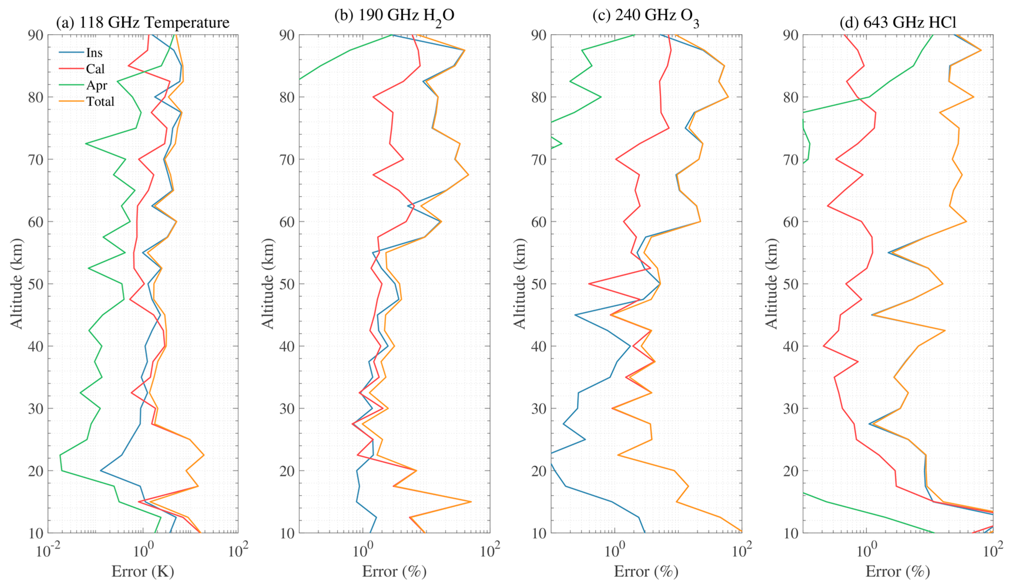
The errors above are simulated independently, keeping the rest of the parameters ideal. The overall error can be calculated by using the sum of the squared errors. R–J approximation is not included, since this error can be avoided by the Planck unit. Figure 21 shows the overall errors of the four radiometers. The errors of temperature are < 3 K from 27 to 57 km. The instrument uncertainties play the most important role above 45 km, while the calibration errors dominate below.
The errors of H2O are < 10% from 16 to 58 km. The instrument uncertainties mainly affect the retrieval above 20 km. The errors of O3 are < 10% from 20 to 58 km, which are similar to that of H2O. The errors of HCl are < 20% from 15 to 59 km which are controlled by instrument uncertainties, while the calibration errors have little impact.
5. Conclusions
The THz Atmospheric Limb Sounder (TALIS) is the first microwave limb sounder being developed in China, and will contribute to atmosphere observation in the future. In this study, the impact of errors on the retrieval induced by three sources including instrument, calibration and external errors, are discussed. Sideband weight, local oscillator offset, measurement noise (NEDT) and pointing angle offset are considered as instrument uncertainties. Calibration errors contain hot target offset, nonlinearity of the two-point calibration, R–J approximation and the antenna pattern. The a priori profiles of temperature, pressure and species are the main external errors, since the model error could not be estimated. It should be noted that simulations from atmospheric profiles under different conditions could have led to different retrieval errors and usable vertical ranges. This simulation only represents a typical atmospheric condition.
Local oscillator offset is quite important in the mesosphere and causes as large as a 5 K error above 50 km. Retrieval error due to the antenna pattern can be as large as 20 K in the troposphere, but less than 3 K at the other altitudes. NEDT, sideband weight and R–J approximation lead to errors of around 1–2 K, respectively. The effect of nonlinearity, hot target offset, pointing offset, pressure and a priori profile are relatively small (<1 K) in the main observation region.
NEDT is the largest error source in 190 GHz H2O retrieval which leads to an error of 10%–40% above 60 km. Local oscillator offset causes as large as a 15% retrieval error at 70 km, but can be neglected below 60 km. R–J approximation is quite important in this frequency band and leads to an error of around 7%. The antenna pattern causes an error of less than 5%, but becomes large in the troposphere. Error due to sideband weight, nonlinearity and hot target offset is less than 1% in the main region, respectively. The effect of pointing offset and a priori profile is quite small.
The results of 240 GHz O3 retrieval are similar to that of 190 GHz. Error induced by NEDT dominates the retrieval in the middle and upper atmosphere. It can lead to the largest error of 50% at 80 km. The error due to R–J approximation is around 10% below 70 km. The impact of the local oscillator is important above 60 km, and this is around 10%. Hot target and nonlinearity are less than 1% below 70 km, respectively. The effect of the antenna pattern is similar to that of 190 GHz. The effect of sideband weight, pointing offset and a priori can be neglected in the main observation region.
The results of 643 GHz have some difference. R–J approximation becomes the largest error source in 643 GHz HCl retrieval. An error of 10%–100% is caused by using R–J approximation in calibration. NEDT causes an error of 10%–50% in the middle and upper atmosphere. Retrieval error induced by the local oscillator is 3%–10% above 60 km, which is similar to other radiometers. Errors due to sideband weight, hot target offset and nonlinearity are less than 1%, respectively. Antenna pattern, pointing offset and a priori are quite small in the main observation region, but become large in the troposphere, since the measurement response is small.
From the simulation above, instrument uncertainties are the most important error sources. The calibration residual errors will affect the retrieval in the troposphere and lower stratosphere. R–J approximation should not be used in calibration unless an additional correction can be done. The a priori uncertainties have little influence. Moreover, it is necessary to use an entire antenna pattern in calibration.
Author Contributions
W.W. performed the simulation and analyzed the results; Z.W. and Y.D. analyzed the error sources; W.W. wrote the manuscript; Z.W. edited the article. All authors have read and agreed to the published version of the manuscript.
Funding
This research received no external funding.
Acknowledgments
The authors would like to thank the ARTS and Qpack development teams for assistance configuring and running the model.
Conflicts of Interest
The authors declare no conflict of interest. The founding sponsors had no role in the design of the study, nor in the collection, analyses, or interpretation of data, as well as no influence in the writing of the manuscript, nor in the decision to publish the results.
References
- Schwartz, M.J.; Lambert, A.; Manney, G.L.; Read, W.G.; Livesey, N.J.; Froidevaux, L.; Ao, C.O.; Bernath, P.F.; Boone, C.D.; Cofield, R.E.; et al. Validation of the Aura Microwave Limb Sounder temperature and geopotential height measurements. J. Geophys. Res. Atmos 2008, 113, D15S11. [Google Scholar] [CrossRef] [Green Version]
- Waters, J.W.; Froidevaux, L.; Read, W.G.; Manney, G.L.; Elson, L.S.; Flower, D.A.; Jarnot, R.F.; Harwood, R.S. Stratospheric ClO and ozone from the Microwave Limb Sounder on the Upper Atmosphere Research Satellite. Nature 1993, 362, 597–602. [Google Scholar] [CrossRef]
- Barath, F.T.; Chavez, M.C.; Cofield, R.E.; Flower, D.A.; Frerking, M.A.; Gram, M.B.; Harris, W.M.; Holden, J.R.; Jarnot, R.F.; Kloezeman, W.G.; et al. The Upper Atmosphere Research Satellite microwave limb sounder instrument. J. Geophys. Res. Atmos. 1993, 98, 10751–10762. [Google Scholar] [CrossRef]
- Waters, J.W.; Read, W.G.; Froidevaux, L.; Jarnot, R.F.; Cofield, R.E.; Flower, D.A.; Lau, G.K.; Pickett, H.M.; Santee, M.L.; Wu, D.L.; et al. The UARS and EOS microwave limb sounder experiments. J. Atmos. Sci. 1999, 56, 194–218. [Google Scholar] [CrossRef] [Green Version]
- Murtagh, D.; Frisk, U.; Merino, F.; Ridal, M.; Jonsson, A.; Stegman, J.; Witt, G.; Eriksson, P.; Jimenez, C.; Mégie, G.; et al. An overview of the Odin atmospheric mission. Can. J. Phys. 2002, 80, 309–319. [Google Scholar] [CrossRef]
- Urban, J.; Lautié, N.; Le Flochmoën, E.; Jiménez, C.; Eriksson, P.; de la Nöe, J.; Dupuy, E.; Ekström, M.; El Amraoui, L.; Frisk, U.; et al. Odin/SMR limb observations of stratospheric trace gases: Level 2 processing of ClO, N2O, HNO3, and O3. J. Geophys. Res. Atmos. 2005, 110, D14307. [Google Scholar] [CrossRef]
- Eriksson, P.; Ekström, M.; Rydberg, B.; Murtagh, D.P. First Odin sub-mm retrievals in the tropical upper troposphere: Ice cloud properties. Atmos. Chem. Phys. 2007, 7, 471–483. [Google Scholar] [CrossRef] [Green Version]
- Frisk, U.; Hagström, M.; Ala-Laurinaho, J.; Andersson, S.; Berges, J.-C.; Chabaud, J.-P.; Dahlgren, M.; Emrich, A.; Florén, H.-G.; Florin, G.; et al. The Odin satellite - I. Radiometer design and test. Astron. Astrophys. 2003, 402, L27–L34. [Google Scholar] [CrossRef] [Green Version]
- Schoeberl, M.R.; Douglass, A.R.; Hilsenrath, E.; Bhartia, P.K.; Beer, R.; Waters, J.W.; Gunson, M.R.; Froidevaux, L.; Gille, J.C.; Barnett, J.J.; et al. Overview of the EOS Aura Mission. IEEE Trans. Geosci. Remote Sens. 2006, 4, 1066–1074. [Google Scholar] [CrossRef] [Green Version]
- Waters, J.W.; Froidevaux, L.; Jarnot, R.F.; Read, W.G.; Pickett, H.M.; Harwood, R.S.; Cofield, R.E.; Filipiak, M.J.; Flower, D.A.; Livesey, N.J.; et al. An Overview of the EOS MLS Experiment, Version 2.0; JPL D-15745/CL# 04-2323; Jet Propulsion Laboratory, California Institute of Technology: Pasadena, CA, USA, 2004. [Google Scholar]
- Waters, J.W.; Froidevaux, L.; Harwood, R.S.; Jarnot, R.F.; Pickett, H.M.; Read, W.G.; Siegel, P.H.; Cofield, R.E.; Filipiak, M.J.; Flower, D.A.; et al. The Earth Observing System Microwave Limb Sounder (EOS MLS) on the Aura Satellite. IEEE Trans. Geosci. Remote Sens. 2006, 44, 1075–1092. [Google Scholar] [CrossRef]
- Wu, D.L.; Schwartz, M.J.; Waters, J.W.; Limpasuvan, V.; Wu, Q.; Killeen, T.L. Mesospheric doppler wind measurements from Aura Microwave Limb Sounder (MLS). Adv. Space Res. 2008, 42, 1246–1252. [Google Scholar] [CrossRef]
- Livesey, N.J.; Logan, J.A.; Santee, M.L.; Waters, J.W.; Doherty, R.M.; Read, W.G.; Froidevaux, L.; Jiang, J.H. Interrelated variations of O3, CO and deep convection in the tropical/subtropical upper troposphere observed by the Aura Microwave Limb Sounder (MLS) during 2004–2011. Atmos. Chem. Phys. 2013, 13, 579–598. [Google Scholar] [CrossRef] [Green Version]
- Wu, D.L.; Jiang, J.H.; Davis, C.P. EOS MLS cloud ice measurements and cloudy-sky radiative transfer model. IEEE Trans. Geosci. Remote Sens. 2006, 44, 1156–1165. [Google Scholar] [CrossRef]
- Kikuchi, K.; Nishibori, T.; Ochiai, S.; Ozeki, H.; Irimajiri, Y.; Kasai, Y.; Koike, M.; Manabe, T.; Mizukoshi, K.; Murayama, Y.; et al. Overview and early results of the Superconducting Submillimeter-Wave Limb-Emission Sounder (SMILES). J. Geophys. Res. Atmos. 2010, 115, D23306. [Google Scholar] [CrossRef]
- Takahashi, C.; Ochiai, S.; Suzuki, M. Operational retrieval algorithms for JEM/SMILES level 2 data processing system. J. Quant. Spectrosc. Ra. 2010, 111, 160–173. [Google Scholar] [CrossRef]
- Baron, P.; Urban, J.; Sagawa, H.; Möller, J.; Murtagh, D.P.; Mendrok, J.; Dupuy, E.; Sato, T.O.; Ochiai, S.; Suzuki, K.; et al. The Level 2 research product algorithms for the Superconducting Submillimeter-Wave Limb-Emission Sounder (SMILES). Atmos. Meas. Tech. 2011, 4, 2105–2124. [Google Scholar] [CrossRef] [Green Version]
- Takahashi, C.; Suzuki, M.; Mitsuda, C.; Ochiai, S.; Manago, N.; Hayashi, H.; Iwata, Y.; Imai, K.; Sano, T.; Takayanagi, M.; et al. Capability for ozone high-precision retrieval on JEM/SMILES observation. Adv. Space Res. 2011, 48, 1076–1085. [Google Scholar] [CrossRef]
- Baron, P.; Murtagh, D.P.; Urban, J.; Sagawa, H.; Ochiai, S.; Kasai, Y.; Kikuchi, K.; Khosrawi, F.; Körnich, H.; Mizobuchi, S.; et al. Observation of horizontal winds in the middle-atmosphere between 30°S and 55°N during the northern winter 2009–2010. Atmos. Chem. Phys. 2013, 13, 6049–6064. [Google Scholar] [CrossRef] [Green Version]
- Jiang, J.H.; Su, H.; Zhai, C.X.; Shen, T.J.; Wu, T.W.; Zhang, J.; Cole, J.N.S.; Salzen, K.V.; Donner, L.J.; Seman, C.; et al. Evaluating the Diurnal Cycle of Upper-Tropospheric Ice Clouds in Climate Models Using SMILES Observations. J. Atmos. Sci. 2015, 72, 1022–1044. [Google Scholar] [CrossRef] [Green Version]
- Baron, P.; Murtagh, D.; Eriksson, P.; Mendrok, J.; Ochiai, S.; Pérot, K.; Sagawa, H.; Suzuki, M. Simulation study for the Stratospheric Inferred Winds (SIW) sub-millimeter limb sounder. Atmos. Meas. Tech. 2018, 11, 4545–4566. [Google Scholar] [CrossRef] [Green Version]
- Ochiai, S.; Baron, P.; Nishibori, T.; Irimajiri, Y.; Uzawa, Y.; Manabe, T.; Maezawa, H.; Mizuno, A.; Nagahama, T.; Sagawa, H.; et al. SMILES-2 Mission for Temperature, Wind, and Composition in the Whole Atmosphere. SOLA 2017, 13A, 13–18. [Google Scholar] [CrossRef] [Green Version]
- Baron, P.; Ochiai, S.; Dupuy, E.; Larsson, R.; Liu, H.X.; Manago, N.; Murtagh, D.; Oyama, S.; Sagawa, H.; Saito, A.; et al. Potential for the measurement of MLT wind, temperature, density and geomagnetic field with Superconducting Submillimeter-Wave Limb-Emission Sounder-2 (SMILES-2). Atmos. Meas. Tech. Discuss. 2019. in review. [Google Scholar]
- Wang, W.Y.; Wang, Z.Z. Performance Evaluation of THz Atmospheric Limb Sounder (TALIS) of China. Atmos. Meas. Technol. 2020, 13, 13–38. [Google Scholar] [CrossRef] [Green Version]
- Verdes, C.; Bühler, S.; von Engeln, A.; Kuhn, T.; Künzi, K.; Eriksson, P.; Sinnhuber, B.M. Pointing and temperature retrieval from millimeter-submillimeter limb soundings. J. Geophys. Res. Atmos. 2002, 107, ACH 10-1–ACH 10-24. [Google Scholar] [CrossRef]
- Eriksson, P.; Ekström, M.; Melsheimer, C.; Buehler, S.A. Efficient forward modelling by matrix representation of sensor responses. Int. J. Remote Sens. 2006, 27, 1793–1808. [Google Scholar] [CrossRef]
- Jarnot, R.F.; Perun, V.S.; Schwartz, M.J. Radiometric and Spectral Performance and Calibration of the GHz Bands of EOS MLS. IEEE Trans. Geosci. Remote Sens. 2006, 44, 1131–1143. [Google Scholar] [CrossRef]
- Ochiai, S.; Kikuchi, K.; Nishibori, T.; Manabe, T. Gain Nonlinearity Calibration of Submillimeter Radiometer for JEM/SMILES. IEEE J. Sel. Top. Appl. Earth Observ. Remote Sens. 2012, 5, 962–969. [Google Scholar] [CrossRef]
- Wang, Z.Z.; Li, J.Y.; He, J.Y.; Zhang, S.W.; Gu, S.Y.; Li, Y.; Guo, Y.; He, B.Y. Performance Analysis of Microwave Humidity and Temperature Sounder Onboard the FY-3D Satellite from Prelaunch Multiangle Calibration Data in Thermal/Vacuum Test. IEEE Trans. Geosci. Remote Sens. 2019, 57, 1664–1683. [Google Scholar] [CrossRef]
- Weng, F.Z.; Zou, X.L. Errors from Rayleigh–Jeans approximation in satellite microwave radiometer calibration systems. Appl. Optics 2013, 52, 505–508. [Google Scholar] [CrossRef]
- Jarnot, R.F.; Cofield, R.E.; Waters, W.G.; Flower, D.A. Calibration of the Microwave Limb Sounder on the Upper Atmosphere Research Satellite. J. Geophys. Res. Atmos. 1996, 101, 9957–9982. [Google Scholar] [CrossRef]
- Cofield, R.E.; Stek, P.C. Design and Field-of-View Calibration of 114–660-GHz Optics of the Earth Observing System Microwave Limb Sounder. IEEE Trans. Geosci. Remote Sens. 2006, 44, 1166–1181. [Google Scholar] [CrossRef]
- Rydberg, B.; Eriksson, P.; Kiviranta, J.; Ringsby, J.; Skyman, A.; Murtagh, D. Odin/SMR Algorithm Theoretical Basis Document: Level 1 Processing. Tech.; Department of Space, Earth and Environment, Chalmers University of Technology: Goteborg, Sweden, 2017. [Google Scholar]
- Rodgers, C.D. Inverse Methods for Atmospheric Sounding: Theory and Practice. World Scientific: Singapore, 2000; pp. 81–99. Available online: https://books.google.com.hk/books?hl=en&lr=&id=FjxqDQAAQBAJ&oi=fnd&pg=PR7&dq=Inverse+Methods+for+Atmospheric+Sounding:+Theory+and+Practice&ots=ARbv5T9AWl&sig=dHFruTHfErcOkyZChZL7PbGHfgU&redir_esc=y&hl=zh-CN&sourceid=cndr#v=onepage&q=Inverse%20Methods%20for%20Atmospheric%20Sounding%3A%20Theory%20and%20Practice&f=false (accessed on 10 December 2019).
- Livesey, N.J.; Snyder, W.V.; Read, W.G.; Wagner, P.A. Retrieval Algorithms for the EOS Microwave Limb Sounder (MLS). IEEE Trans. Geosci. Remote Sens. 2006, 44, 1144–1155. [Google Scholar] [CrossRef]
- Erikson, P.; Chen, D. Statistical parameters derived from ozonesonde data of importance for passive remote sensing observations of ozone. Int. J. Remote. Sens. 2002, 23, 4945–4963. [Google Scholar] [CrossRef]
- Rodgers, C.D. Characterization and error analysis of profilesretrieved from remote sounding measurements. J. Geophys. Res. 1990, 95, 5587–5595. [Google Scholar] [CrossRef]
- Eriksson, P.; Buehler, S.A.; Davis, C.P.; Emde, C.; Lemke, O. ARTS, the atmospheric radiative transfer simulator, Version 2. J. Quant. Spectrosc. Ra. 2011, 112, 1551–1558. [Google Scholar] [CrossRef] [Green Version]
- Eriksson, P.; Jiménez, C.; Buehler, S.A. Qpack, a general tool for instrument simulation and retrieval work. J. Quant. Spectrosc. Ra. 2005, 91, 47–64. [Google Scholar] [CrossRef] [Green Version]
Figure 1.
Schematic of two-point calibration.
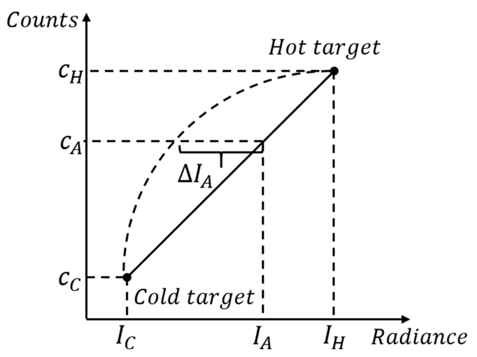
Figure 2.
The variations of calibration errors with temperature and the count ratio induced by the R–J approximation: (a) variations with temperature; (b) variations with the count ratio. Here is calculated by Equation (3), and is obtained from replacing by with and set to 2.73 and 300 K, respectively. The count ratio means .
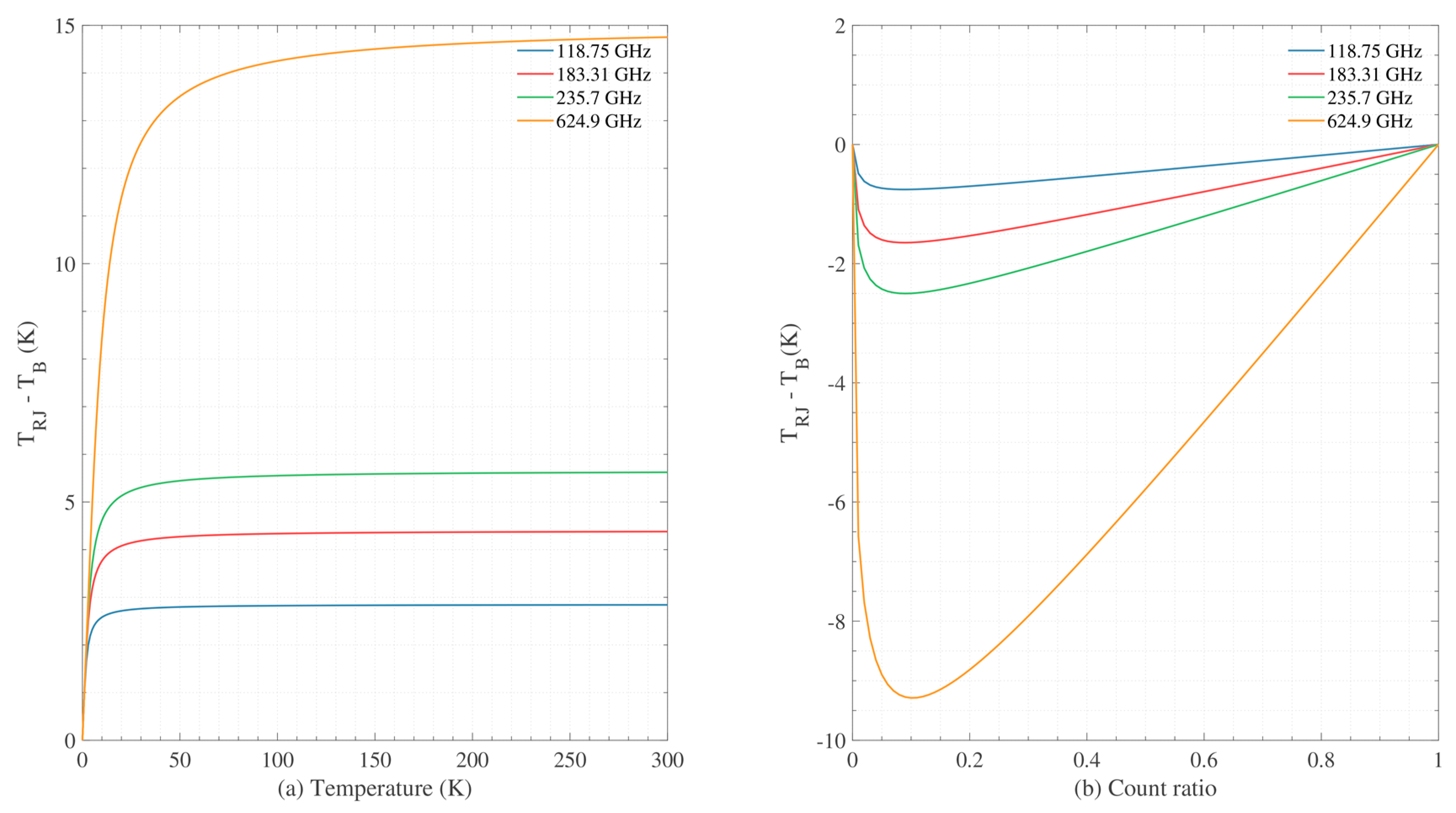
Figure 3.
The antenna pattern of TALIS: (a) the 118 GHz antenna pattern; (b) the 190 GHz antenna pattern; (c) the 240 GHz antenna pattern; (d) the 643 GHz antenna pattern.
Figure 3.
The antenna pattern of TALIS: (a) the 118 GHz antenna pattern; (b) the 190 GHz antenna pattern; (c) the 240 GHz antenna pattern; (d) the 643 GHz antenna pattern.
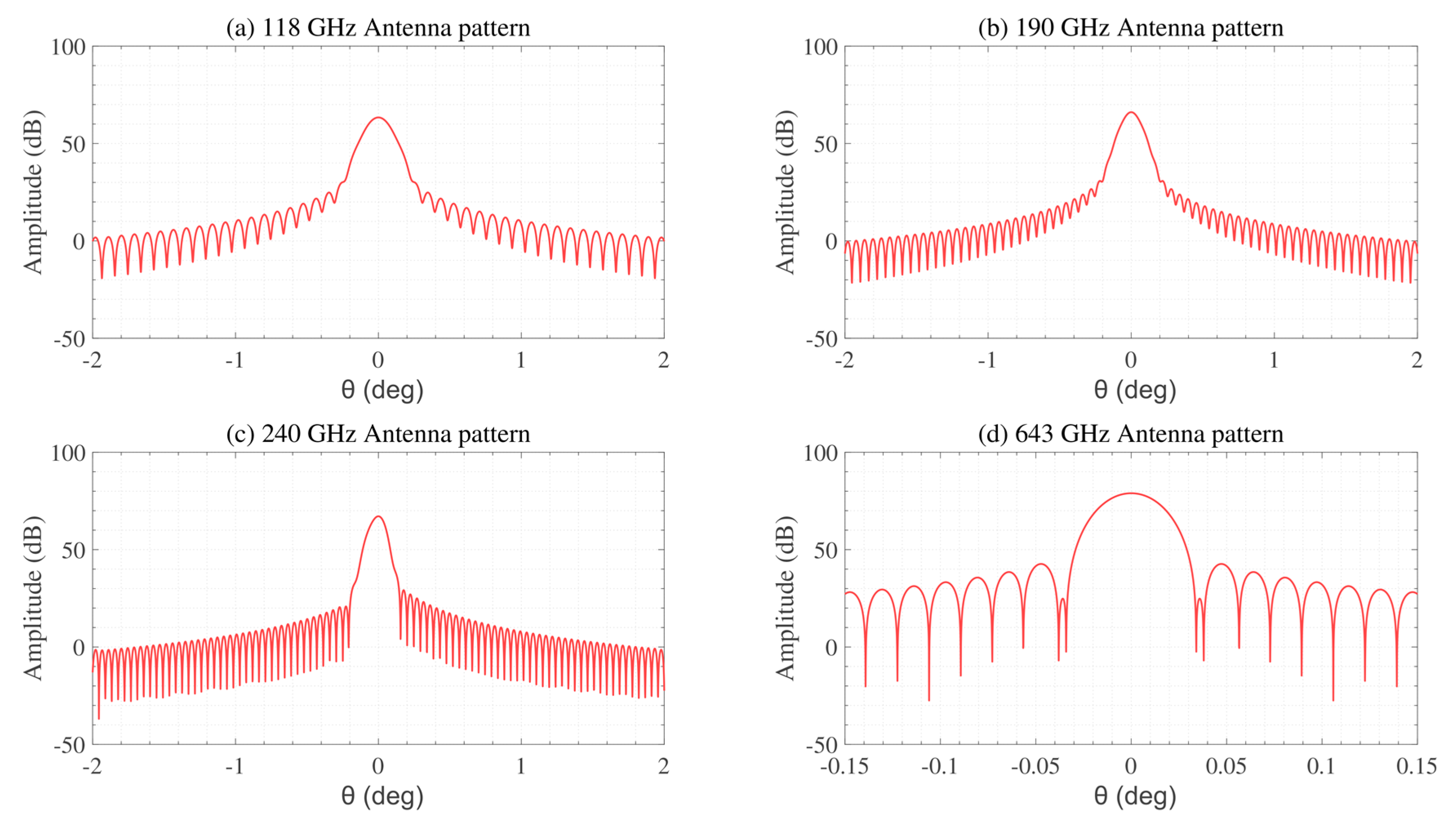
Figure 4.
The retrieval precision of the four radiometers with different retrieval grids, and only random noises are added: (a) 118 GHz temperature retrieval; (b) 190 GHz H2O retrieval; (c) 240 GHz O3 retrieval; (d) 643 GHz HCl retrieval. The 1 km, 2.5 km, 5 km represent the different retrieval grids. The “Profile” represents the typical profile.
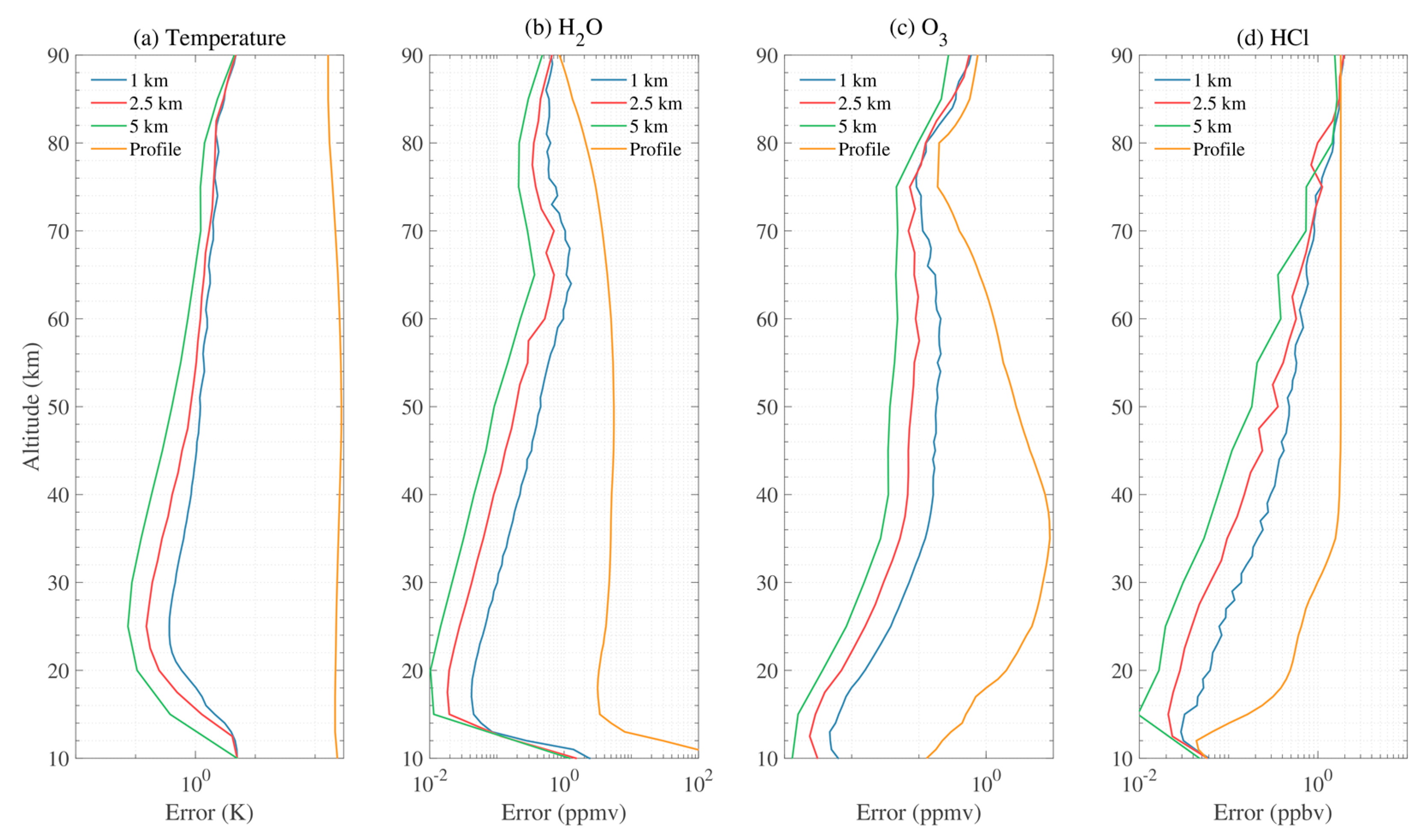
Figure 5.
The temperature retrieval errors induced by different instrument uncertainty sources: (a) absolute and (b) relative retrieval errors. The uncertainties assumed are summarized in Table 3.
Figure 5.
The temperature retrieval errors induced by different instrument uncertainty sources: (a) absolute and (b) relative retrieval errors. The uncertainties assumed are summarized in Table 3.
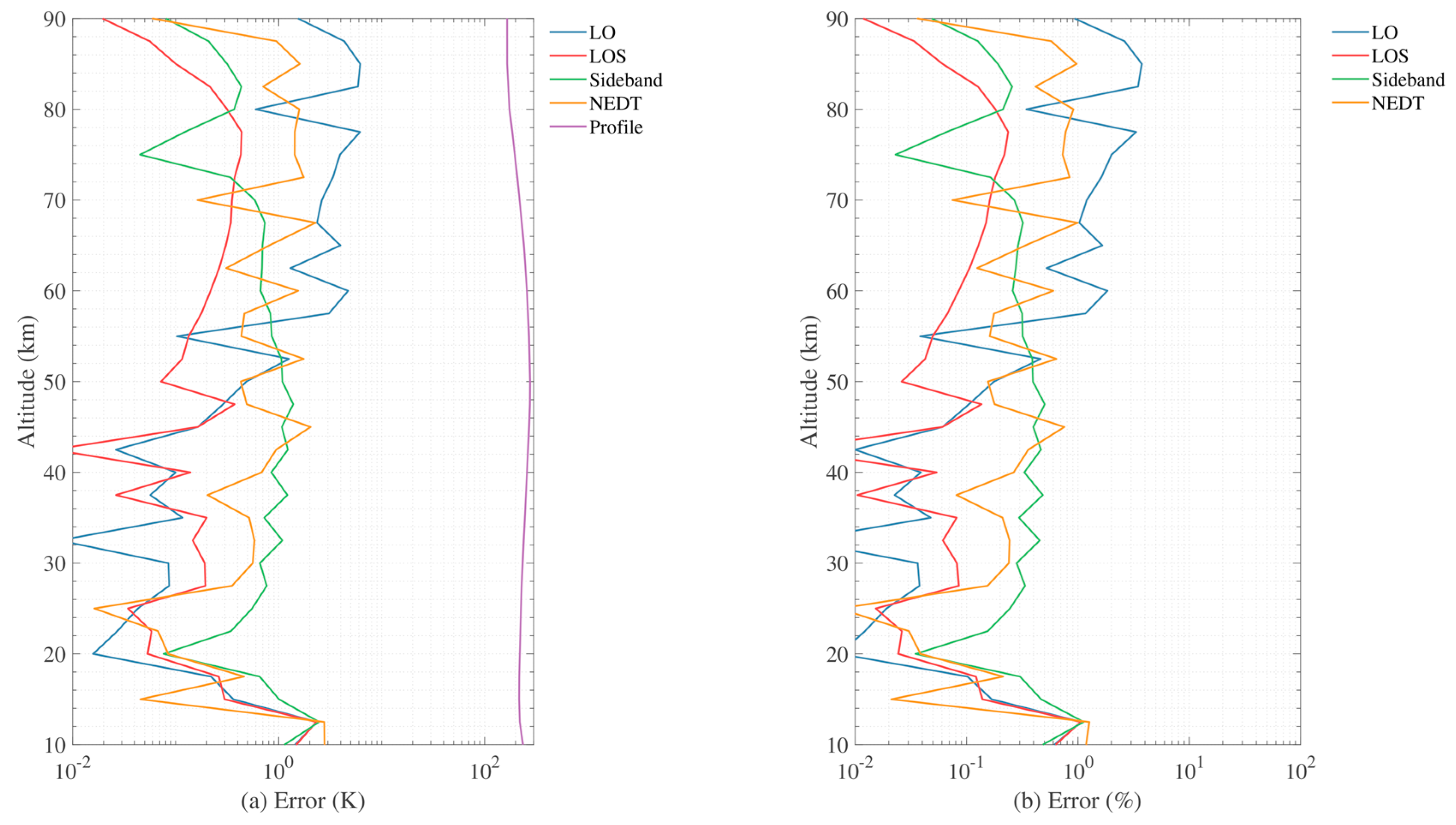
Figure 6.
The brightness temperature difference − at various tangent height measured by the 118 GHz radiometer: (a) 10 km; (b) 20 km; (c) 30 km; (d) 50 km; (e) 70 km; (f) 90 km.
Figure 6.
The brightness temperature difference − at various tangent height measured by the 118 GHz radiometer: (a) 10 km; (b) 20 km; (c) 30 km; (d) 50 km; (e) 70 km; (f) 90 km.

Figure 7.
The temperature retrieval errors induced by different calibration error sources: (a) absolute and (b) relative retrieval errors. The uncertainties assumed are summarized in Table 4.
Figure 7.
The temperature retrieval errors induced by different calibration error sources: (a) absolute and (b) relative retrieval errors. The uncertainties assumed are summarized in Table 4.
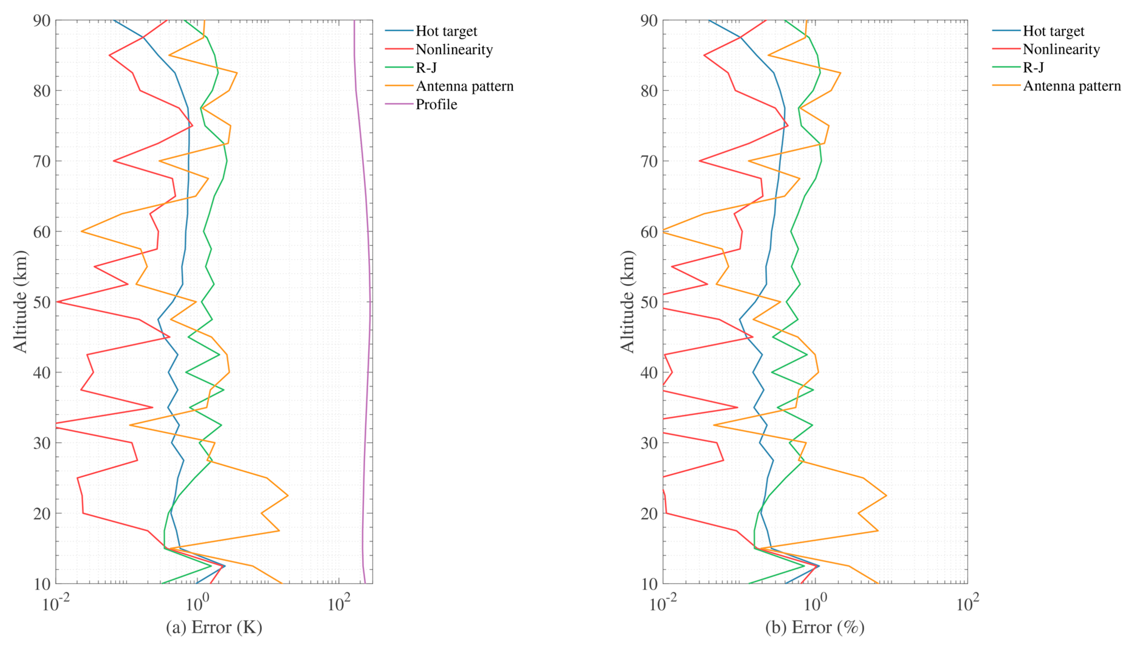
Figure 8.
The temperature retrieval errors induced by external error sources: (a) absolute and (b) relative retrieval errors. The uncertainties assumed are summarized in Table 5.
Figure 8.
The temperature retrieval errors induced by external error sources: (a) absolute and (b) relative retrieval errors. The uncertainties assumed are summarized in Table 5.
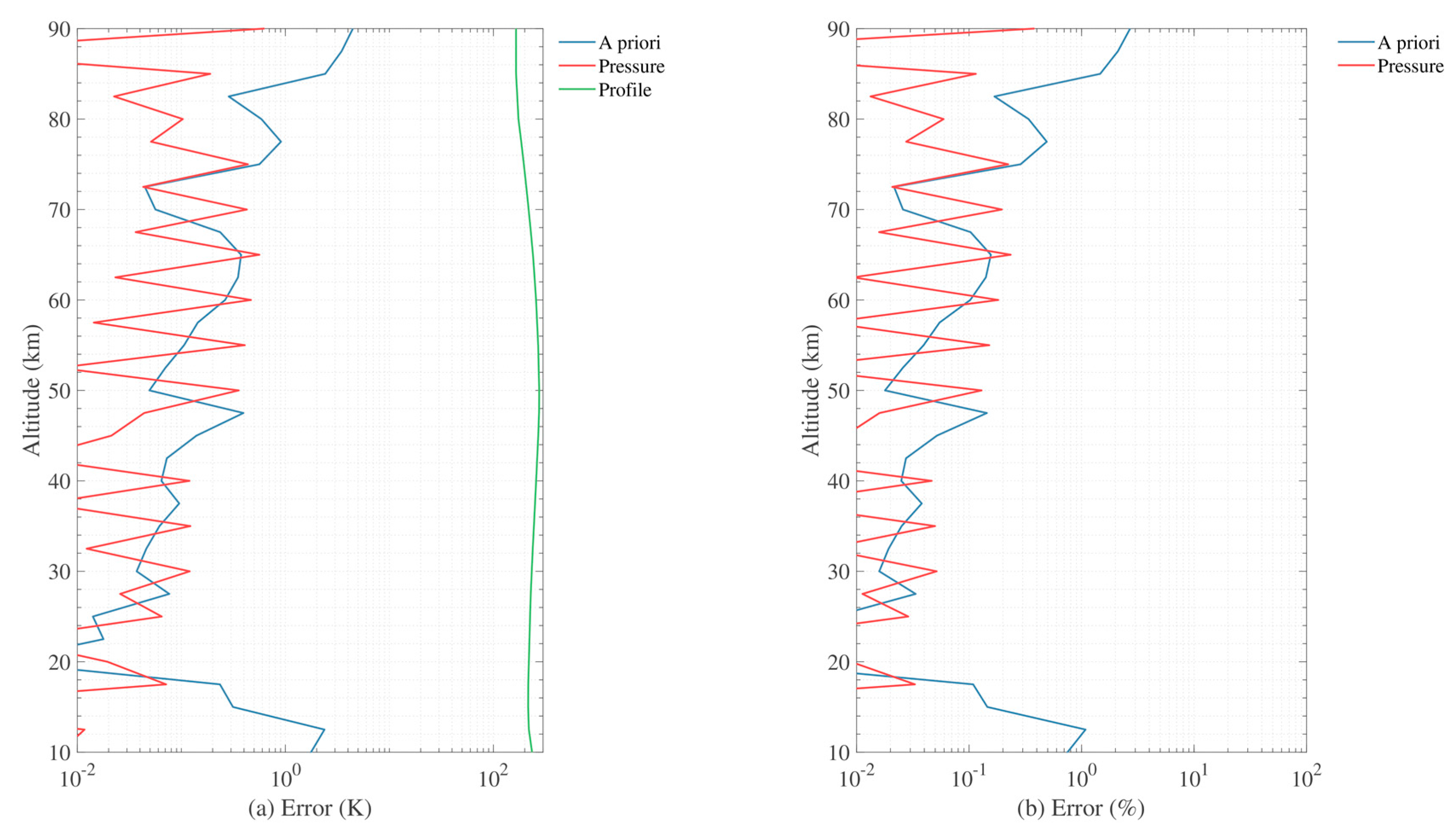
Figure 9.
The H2O retrieval errors induced by different instrument uncertainty sources: (a) absolute and (b) relative retrieval errors. The uncertainties assumed are summarized in Table 3.
Figure 9.
The H2O retrieval errors induced by different instrument uncertainty sources: (a) absolute and (b) relative retrieval errors. The uncertainties assumed are summarized in Table 3.
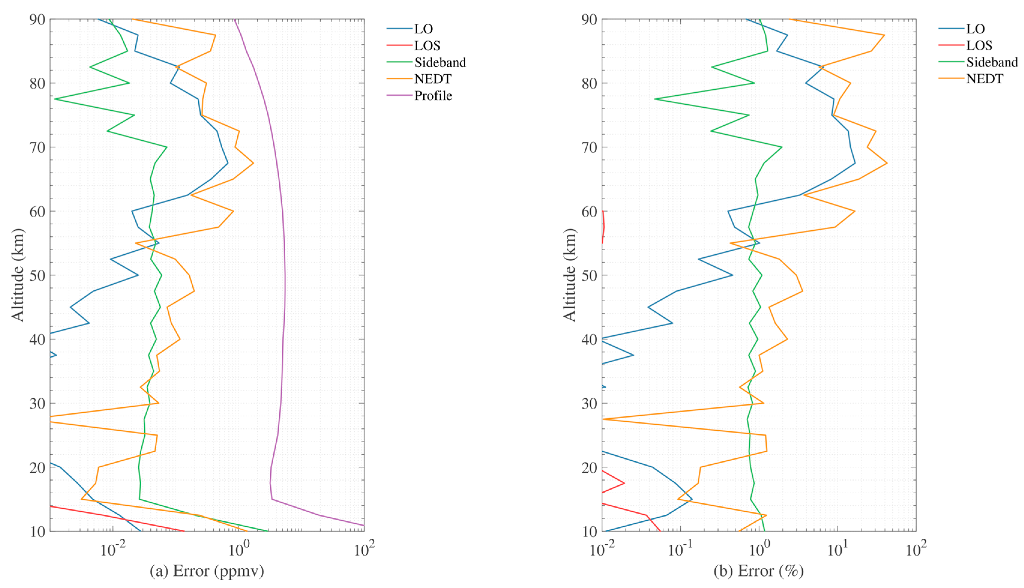
Figure 10.
The brightness temperature difference − at various tangent height measured by 190 GHz radiometer (183 GHz spectrometer): (a) 10 km; (b) 20 km; (c) 30 km; (d) 50 km; (e) 70 km; (f) 90 km.
Figure 10.
The brightness temperature difference − at various tangent height measured by 190 GHz radiometer (183 GHz spectrometer): (a) 10 km; (b) 20 km; (c) 30 km; (d) 50 km; (e) 70 km; (f) 90 km.

Figure 11.
The H2O retrieval errors induced by different calibration error sources: (a) absolute and (b) relative retrieval errors. The uncertainties assumed are summarized in Table 4.
Figure 11.
The H2O retrieval errors induced by different calibration error sources: (a) absolute and (b) relative retrieval errors. The uncertainties assumed are summarized in Table 4.
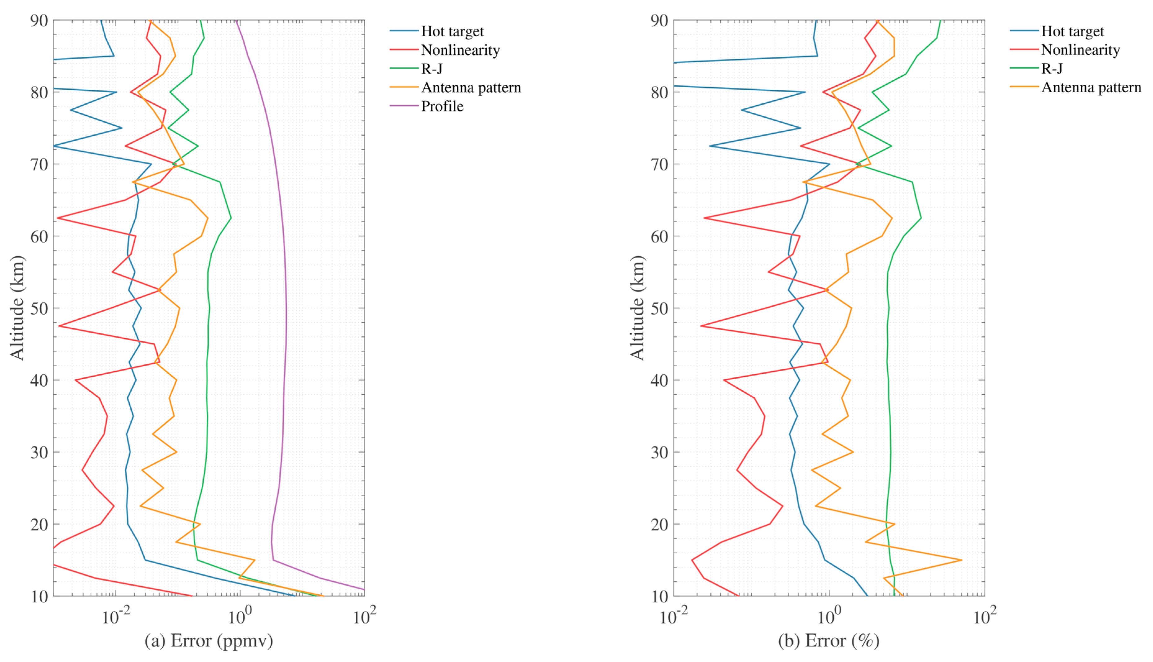
Figure 12.
The H2O retrieval error induced by external error source: (a) absolute and (b) relative retrieval errors. The uncertainties assumed are summarized in Table 5.
Figure 12.
The H2O retrieval error induced by external error source: (a) absolute and (b) relative retrieval errors. The uncertainties assumed are summarized in Table 5.

Figure 13.
The O3 retrieval errors induced by different instrument uncertainty sources: (a) absolute and (b) relative retrieval errors. The uncertainties assumed are summarized in Table 3.
Figure 13.
The O3 retrieval errors induced by different instrument uncertainty sources: (a) absolute and (b) relative retrieval errors. The uncertainties assumed are summarized in Table 3.

Figure 14.
The brightness temperature difference TA − TB at various tangent height measured by 240 GHz radiometer (235 GHz spectrometer): (a) 10 km; (b) 20 km; (c) 30 km; (d) 50 km; (e) 70 km; (f) 90 km.
Figure 14.
The brightness temperature difference TA − TB at various tangent height measured by 240 GHz radiometer (235 GHz spectrometer): (a) 10 km; (b) 20 km; (c) 30 km; (d) 50 km; (e) 70 km; (f) 90 km.
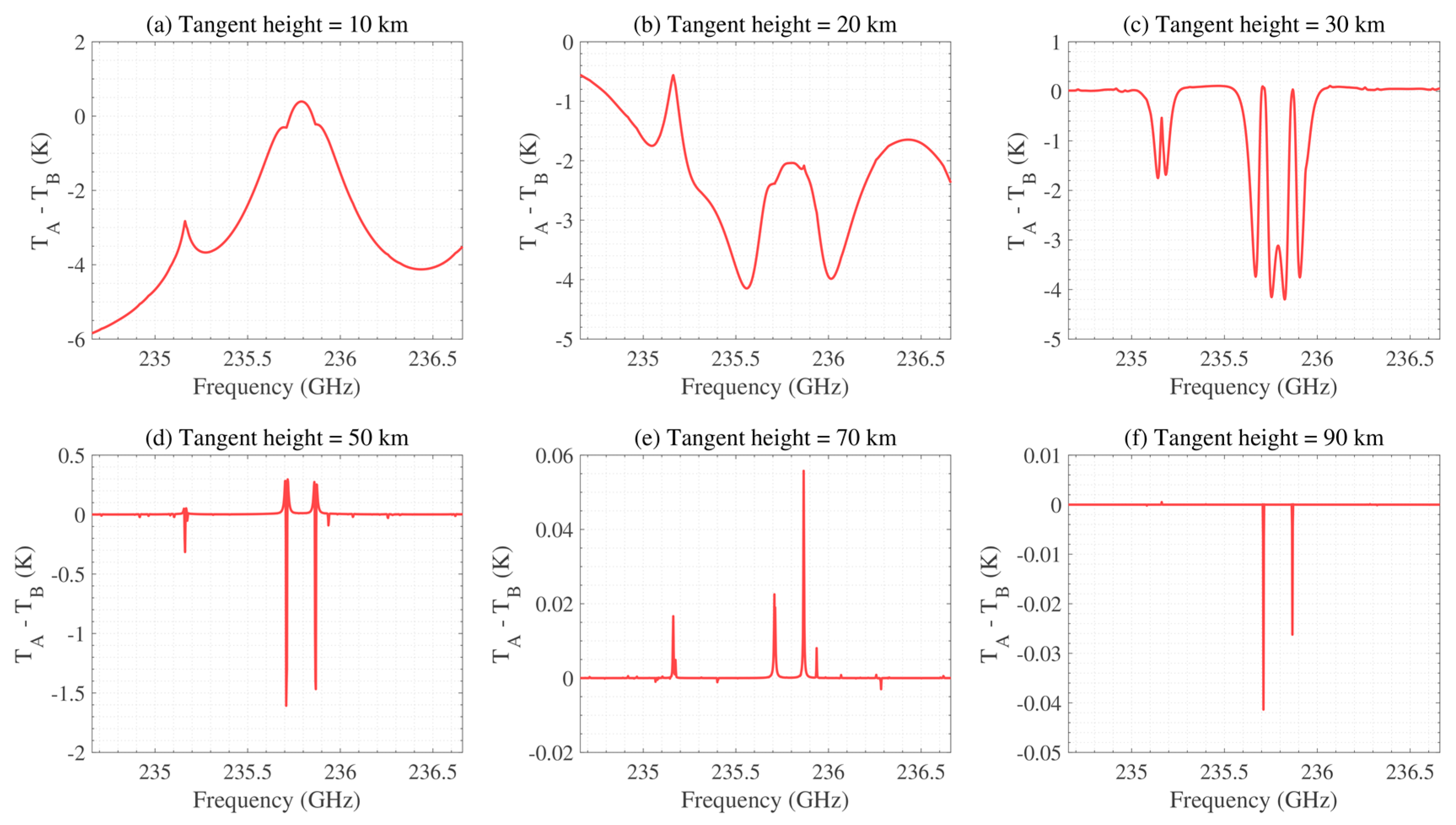
Figure 15.
The O3 retrieval errors induced by different calibration error sources: (a) absolute and (b) relative retrieval errors. The uncertainties assumed are summarized in Table 4.
Figure 15.
The O3 retrieval errors induced by different calibration error sources: (a) absolute and (b) relative retrieval errors. The uncertainties assumed are summarized in Table 4.

Figure 16.
The O3 retrieval error induced by external error source: (a) absolute and (b) relative retrieval errors. The uncertainties assumed are summarized in Table 5.
Figure 16.
The O3 retrieval error induced by external error source: (a) absolute and (b) relative retrieval errors. The uncertainties assumed are summarized in Table 5.
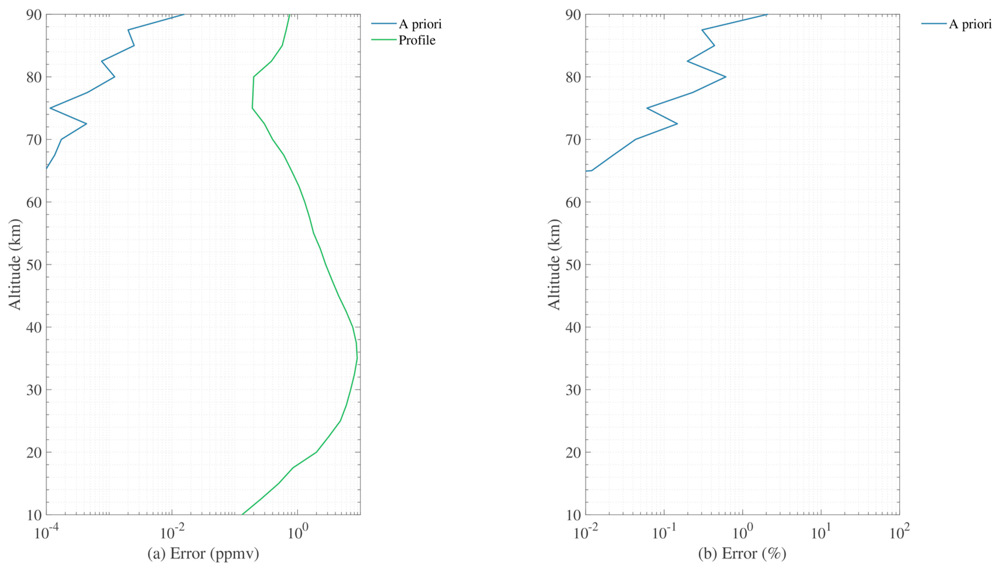
Figure 17.
The HCl retrieval errors induced by different instrument uncertainty sources: (a) absolute and (b) relative retrieval errors. The uncertainties assumed are summarized in Table 3.
Figure 17.
The HCl retrieval errors induced by different instrument uncertainty sources: (a) absolute and (b) relative retrieval errors. The uncertainties assumed are summarized in Table 3.
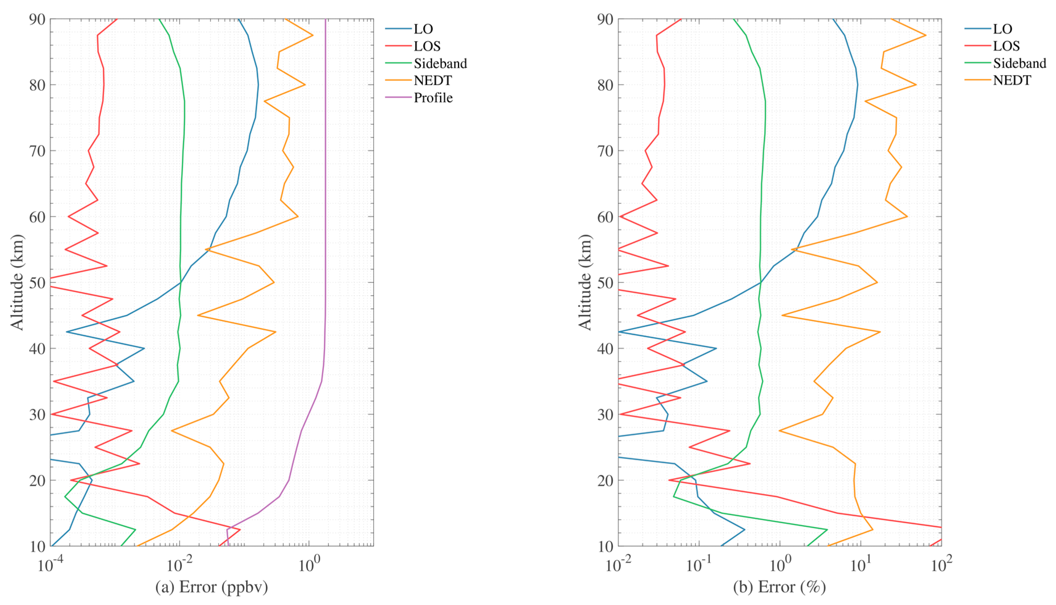
Figure 18.
The brightness temperature difference − at various tangent height measured by 643 GHz radiometer (625 GHz spectrometer): (a) 10 km; (b) 20 km; (c) 30 km; (d) 50 km; (e) 70 km; (f) 90 km.
Figure 18.
The brightness temperature difference − at various tangent height measured by 643 GHz radiometer (625 GHz spectrometer): (a) 10 km; (b) 20 km; (c) 30 km; (d) 50 km; (e) 70 km; (f) 90 km.
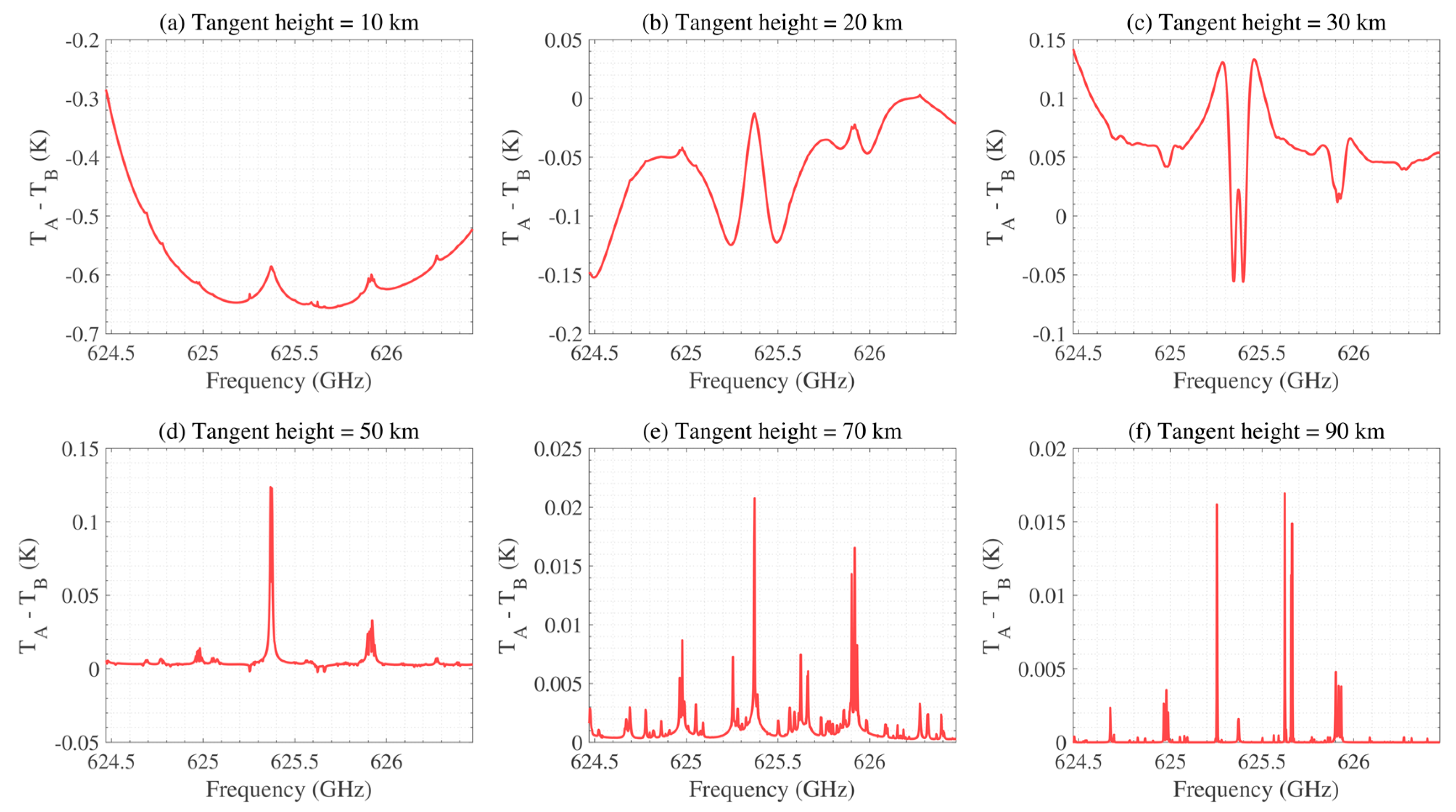
Figure 19.
The HCl retrieval errors induced by different calibration error sources: (a) absolute and (b) relative retrieval errors. The uncertainties assumed are summarized in Table 4.
Figure 19.
The HCl retrieval errors induced by different calibration error sources: (a) absolute and (b) relative retrieval errors. The uncertainties assumed are summarized in Table 4.

Figure 20.
The HCl retrieval error induced by external error source: (a) absolute and (b) relative retrieval errors. The uncertainties assumed are summarized in Table 5.
Figure 20.
The HCl retrieval error induced by external error source: (a) absolute and (b) relative retrieval errors. The uncertainties assumed are summarized in Table 5.
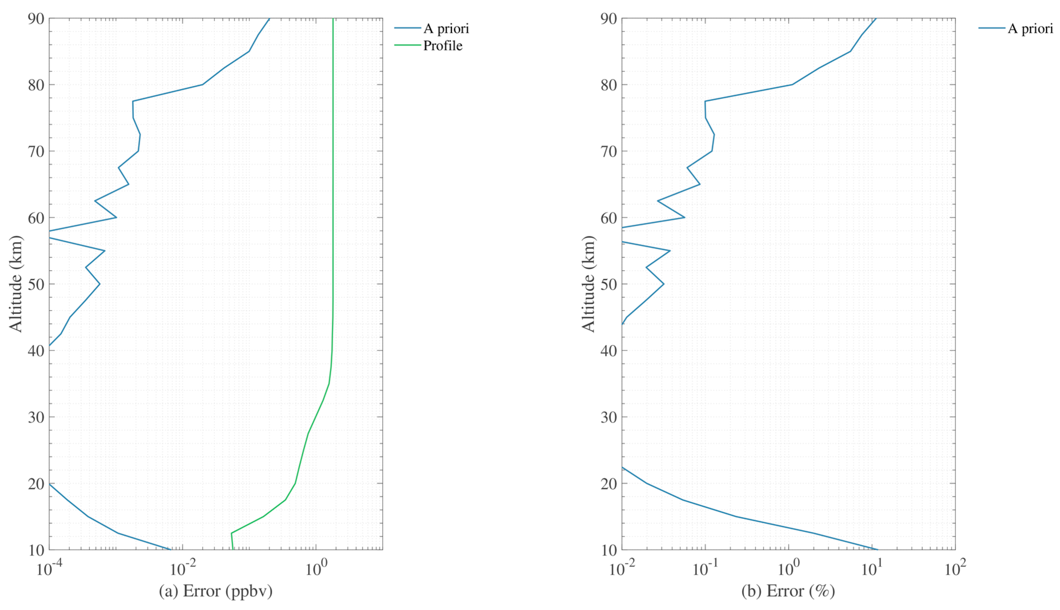
Figure 21.
The overall retrieval errors estimation: (a) 118 GHz temperature retrieval; (b) 190 GHz H2O retrieval; (c) 240 GHz O3 retrieval; (d) 643 GHz HCl retrieval. The errors are calculated by using the sum of squared errors.
Figure 21.
The overall retrieval errors estimation: (a) 118 GHz temperature retrieval; (b) 190 GHz H2O retrieval; (c) 240 GHz O3 retrieval; (d) 643 GHz HCl retrieval. The errors are calculated by using the sum of squared errors.

Table 1.
The main observation characteristics of the THz Atmospheric Limb Sounder (TALIS).
| Characteristics | Value |
|---|---|
| Satellite altitude | 600 km |
| Scan altitude | 0–100 km |
| Spectrum integration time | 0.1 s (1 km) |
| Antenna vertical FOV | 5.5 km, 3.8 km, 3.3 km, 0.96 km |
| Spectrometer bandwidth | 2 GHz |
| Spectrometer resolution | 2 MHz |
| Local oscillator frequency | 117.55, 190.1, 239.66, 642.87 GHz |
Table 2.
The spectral bands of the TALIS.
| Radiometer (GHz) | Spectral Bands (GHz) | System Temperature (K) |
|---|---|---|
| 118 | 115.35–117.35, 117.75–119.75 | 1000 K, DSB |
| 190 | 175.5–177.5, 202.7–204.7; 178.9–180.9, 199.3–201.3; 183.0–185.0, 195.2–197.2 | 1000 K, DSB |
| 240 | 229.66–231.66, 247.66–249.66; 232.16–234.16, 245.16–247.16; 234.66–236.66, 242.66–244.66 | 1000 K, DSB |
| 643 | 624.47–626.47, 659.27–661.27; 627.37–629.37, 656.37–658.37; 632.37–634.37, 651.37–653.37; 634.87–636.87, 648.87–650.87 | 2300 K, DSB |
Table 3.
Uncertainties assumed for instrument.
| Source | Value |
|---|---|
| Sideband weight | 0.2% |
| Local oscillator | 0.5 MHz |
| Pointing offset (LOS) | 0.021° |
| Measurement noise (NEDT) | 2.2 K, 2.2 K, 2.2 K, 5.1 K |
Table 4.
Errors assumed for calibration.
| Source | Value |
|---|---|
| Hot target offset | −0.5 K |
| Nonlinearity | 0.3 K |
| R–J approximation | / |
| Antenna pattern used | 3 dB FWHM |
Table 5.
Uncertainties assumed for external errors.
| Source | Value |
|---|---|
| Temperature a priori | 5 K |
| Pressure a priori | 5% |
| Species a priori | 20% |
© 2020 by the authors. Licensee MDPI, Basel, Switzerland. This article is an open access article distributed under the terms and conditions of the Creative Commons Attribution (CC BY) license (http://creativecommons.org/licenses/by/4.0/).
Share and Cite
MDPI and ACS Style
Wang, W.; Wang, Z.; Duan, Y. Preliminary Evaluation of the Error Budgets in the TALIS Measurements and Their Impact on the Retrievals. Remote Sens. 2020, 12, 468. https://doi.org/10.3390/rs12030468
AMA Style
Wang W, Wang Z, Duan Y. Preliminary Evaluation of the Error Budgets in the TALIS Measurements and Their Impact on the Retrievals. Remote Sensing. 2020; 12(3):468. https://doi.org/10.3390/rs12030468
Chicago/Turabian StyleWang, Wenyu, Zhenzhan Wang, and Yongqiang Duan. 2020. "Preliminary Evaluation of the Error Budgets in the TALIS Measurements and Their Impact on the Retrievals" Remote Sensing 12, no. 3: 468. https://doi.org/10.3390/rs12030468
Note that from the first issue of 2016, this journal uses article numbers instead of page numbers. See further details here.