Article

Precipitation and Minimum Temperature are Primary Climatic Controls of Alpine Grassland Autumn Phenology on the Qinghai-Tibet Plateau

1
College of Applied Arts and Science, Beijing Union University, Beijing 100191, China
2
Laboratory for Earth Surface Processes of the Ministry of Education, College of Urban and Environmental Sciences, Peking University, Beijing 100871, China
3
Geospatial Sciences Center of Excellence (GSCE), South Dakota State University, Brookings, SD 57007, USA
4
Department of Geography & Geospatial Sciences, South Dakota State University, Brookings, SD 57007, USA
5
Environment Research Institute, Shandong University, Qingdao 266237, China
6
College of Resources and Environmental Sciences, China Agricultural University, Beijing 100193, China
*
Author to whom correspondence should be addressed.
Remote Sens. 2020, 12(3), 431; https://doi.org/10.3390/rs12030431
Submission received: 27 December 2019 / Revised: 24 January 2020 / Accepted: 26 January 2020 / Published: 29 January 2020

Abstract

:
Autumn phenology is a crucial indicator for identifying the alpine grassland growing season’s end date on the Qinghai-Tibet Plateau (QTP), which intensely controls biogeochemical cycles in this ecosystem. Although autumn phenology is thought to be mainly influenced by the preseason temperature, precipitation, and insolation in alpine grasslands, the relative contributions of these climatic factors on the QTP remain uncertain. To quantify the impacts of climatic factors on autumn phenology, we built stepwise linear regression models for 91 meteorological stations on the QTP using in situ herb brown-off dates, remotely sensed autumn phenological metrics, and a multi-factor climate dataset during an optimum length period. The results show that autumn precipitation has the most extensive influence on interannual variation in alpine grassland autumn phenology. On average, a 10 mm increase in autumn precipitation during the optimum length period may lead to a delay of 0.2 to 4 days in the middle senescence date (P < 0.05) across the alpine grasslands. The daily minimum air temperature is the second most important controlling factor, namely, a 1 °C increase in the mean autumn minimum temperature during the optimum length period may induce a delay of 1.6 to 9.3 days in the middle senescence date (P < 0.05) across the alpine grasslands. Sunshine duration is the third extensive controlling factor. However, its influence is spatially limited. Moreover, the relative humidity and wind speed also have strong influences at a few stations. Further analysis indicates that the autumn phenology at stations with less autumn precipitation is more sensitive to precipitation variation than at stations with more autumn precipitation. This implies that autumn drought in arid regions would intensely accelerate the leaf senescence of alpine grasslands. This study suggests that precipitation should be considered for improving process-based autumn phenology models in QTP alpine grasslands.

Graphical Abstract

1. Introduction

As the “third pole” of the earth, the Qinghai-Tibet Plateau (QTP) has attracted much attention from the scientific community because of its unique alpine environment. During the past half century, the QTP has undergone significant warming at a rate twice the global average [1]. Alpine grassland is the dominant QTP vegetation type, occupying more than 60% of the total area. Thus, rapid warming has resulted in a remarkable change of the vegetation phenology in the alpine grassland, such as the advancement of spring phenology [2,3,4,5,6], the delay of autumn phenology [4,7,8], and growing season extension [9]. These changes will inevitably have a significant impact on the structure and function of the alpine grassland ecosystem [10]. As an important time marker, autumn phenology directly indicates the end date of the growing season and determines (together with spring phenology) the growing season length, which in turn may have significant impacts on the biomass accumulation, atmospheric exchange of trace gases, and biogeochemical cycles of the terrestrial ecosystem [11,12,13]. Revealing the development process and its climate controls of alpine grassland autumn phenology can therefore not only contribute to an improvement of the phenology modules in ecosystem models but also enhance the ability to predict alpine grassland growing seasons, biomass, and carbon cycles under future climate change scenarios [14].
The relationships between plant autumn phenology and climatic factors are more complicated than with the spring phenology [15] and its mechanisms are still not clear [14,16,17]. Based on partial correlation or regression analysis, temperature, precipitation, and insolation are considered to be important climatic factors affecting the autumn phenology of herbaceous plants on the QTP [7,8,18,19]. However, the relative importance of each factor is not known. Among them, temperature is commonly thought to be the most important driver; the higher the average preseason temperature, the later the autumn phenology [7,8,19,20,21]. Precipitation and sunshine duration are secondary influence factors, but the results from different studies are inconsistent. There are two opposite conclusions: Higher preseason precipitation could lead to either later [7,19,22] or earlier autumn phenology [8,21]; longer sunshine duration could also result in earlier [7] or later [19] autumn phenology. Furthermore, although the statistical relationship between the air temperature and autumn phenology of alpine grassland is relatively clear, different temperature indexes have different effects on autumn phenology. Specifically, daytime and nighttime temperatures have different impacts on alpine grassland autumn phenology [11,23]. Increased nighttime temperatures generally postpone autumn grassland phenology, while increased daytime temperatures typically advance it [23]. However, the relative contributions of daytime and nighttime temperatures to autumn phenology are not well understood.
In addition to temperature, precipitation, and sunshine, strong winds could also affect autumn phenological variations [12], because they could enhance ground surface evaporation and air humidity, and reduce surface temperature. However, the effects of wind speed and relative humidity on autumn phenology are poorly understood [12]. In this study, we explored the effects of daily minimum/maximum/mean air temperature, daily precipitation, daily sunshine duration, daily mean relative humidity, daily mean/maximum wind speed, and their interactions on QTP alpine grassland autumn phenology. Then, we identified their relative contributions based on the sphere of influence of each climatic factor to alpine grassland autumn phenology.

2. Materials and Methods

The processing sequence for analyzing autumn phenology is shown in Figure 1. Details are illustrated in the following sections.

2.1. Study Area

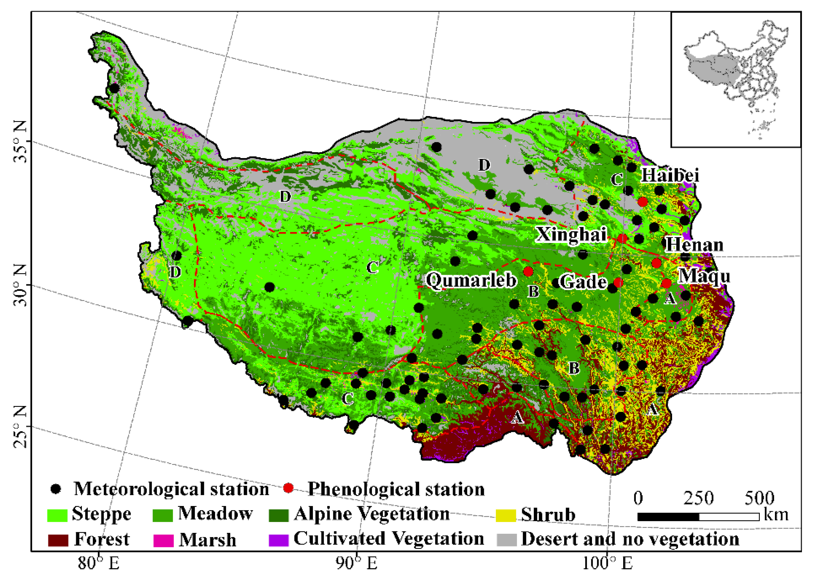
The QTP is mainly located in China, including Qinghai Province, the Tibet Autonomous Region, western Sichuan Province, and parts of Yunnan Province, Xinjiang Uygur Autonomous Region, and Gansu Province. The eastern and southeastern parts of the QTP are affected mainly by the south Asia monsoon in summer and prevailing westerlies in winter. From southeast to northwest, the annual mean air temperature is between 15.5 and −5 °C, while the annual accumulated precipitation has been between 1764 and 16 mm over the past three decades [5]. Unique vegetation types have evolved on the QTP in response to its special alpine environment (Figure 2), mainly containing steppe, meadow, and alpine vegetation. Specifically, steppe is mainly composed of the carex high-cold steppe, while meadow is mainly made up of the kobresia high-cold meadow. Alpine vegetation contains different vegetation types, such as alpine tundra, sparse vegetation, and alpine cushion vegetation. Other vegetation types with small distribution ranges include broad-leaved and coniferous forests, shrub, and cultivated vegetation [24].

2.2. Phenological and Metrological Data

Field observation data for the brown-off date were obtained from the China Meteorological Administration, including 19 herb species at 6 phenological stations over 2000 to 2012. Each phenological station is in a natural pasture with a fenced area of 10,000 m2. Phenological observations were carried out every 2 days for 10 individual herbaceous plants of each species in a selected 1 m × 1 m grassland quadrat by professionals according to uniform observation criteria [25]. The brown-off date was determined as the day when the leaves turn brown in two thirds of individual herbaceous plants. The observation objects include local dominant species, such as poaceae, leguminosae, and cyperaceae, and accompanying species, such as compositae, chenopodiaceae, liliaceous, rosaceae, umbrella, and labiatae (Table S1). The mean brown-off dates from multi-species at each station were used to validate the reliability of the remotely sensed autumn phenology.
Meteorological data were derived from the China Meteorological Data Sharing Service System in the China Meteorological Administration (http://www.nmic.cn/). The data include the daily minimum/maximum/mean air temperature, daily precipitation, daily sunshine duration, daily mean relative humidity, and daily mean/maximum wind speed from 2000 to 2015 at 91 stations in alpine grasslands (Figure 2). Meteorological stations are located at elevations ranging from 1583.3 to 4900 m.

2.3. Land Surface Autumn Phenology Datasets

Land surface autumn phenology from 2000 to 2015 was extracted based on the Moderate Resolution Imaging Spectroradiometer (MODIS) Nadir Bidirectional Reflectance Distribution Function (BRDF)-Adjusted Reflectance (NBAR) dataset (MCD43A4 Version 6) [27] and Albedo Quality Product (MCD43A2) [28]. The spatial resolution is 500 m and the temporal resolution is one day. Both MCD43A4 and MCD43A2 products were downloaded from the National Aeronautics and Space Administration (NASA) website (http://modis.gsfc.nasa.gov/). The daily normalized difference vegetation index (NDVI) and 2-band enhanced vegetation index (EVI2) were calculated from MCD43A4 using Equations (1) and (2):
NDVI = ( N I R R ) ( N I R + R ) ,
EVI 2 = 2.5 N I R R N I R + 2.4 R + 1 ,  
where NIR and R are the NBAR of the near infrared and red band, respectively.
NDVI has generally been used to estimate vegetation phenology in previous research. However, NDVI is easily saturated in higher vegetation cover, while EVI2 has recently shown a better performance [29,30]. Thus, we used both NDVI and EVI2 to extract autumn phenology and compared the results. To do this, NDVI and EVI2 time series were fitted using the vegetation growing curve described in a logistic model, and the curvature change rate was calculated to identify the phenological transition dates [31,32]. Specifically, a hybrid piecewise logistic model (HPLM) algorithm was used to describe the temporal NDVI/EVI2 trajectory. Method details can be found in the existing literature [33,34]. Based on the HPLM and curvature change rates, a set of phenological metrics were identified. During a senescence period, there are three extreme points (two minimum and one maximum values) in the curvature change rate, where the two minimum extreme points correspond to senescence onset and dormancy onset, separately, while the maximum point corresponds to the date at the mid-senescent phase that is close to 50% of the total seasonal amplitude [34]. The autumn phenology occurrence date in our research is defined as the middle senescence date (MSD) (Figure 3), which is identified using the maximum extreme point in the curvature change rate of HPLM [34]. It should be noted that only the first growing cycle of grassland is addressed in this study if there are two or more growing cycles. In fact, there is only one growing season for most of the alpine grassland on the QTP, due to its special alpine climate.

2.4. Validation of the Remotely Sensed Middle Senescence Date

To select the best spatial scale of the remotely sensed MSD reflecting the ground-observed autumn phenology, we evaluated MSD at different spatial scales using multi-species mean brown-off dates observed at the ground stations. The evaluation indices the are mean absolute error (MAE, Equation (3)), root mean square error (RMSE, Equation (4)), and Pearson correlation coefficient (r, Equation (5)):
M A E = 1 n i = 1 n | x i y i | ,
R M S E = i = 1 n ( x i y i ) 2 n ,
r = i = 1 n ( x i x ¯ ) ( y i y ¯ ) i = 1 n ( x i x ¯ ) 2 i = 1 n ( y i y ¯ ) 2 ,
where i is the sequence number of the year, n is the total number of years, x i is the mean brown-off date of multi species from ground observations at a station in the i-th year, y i is the remotely sensed middle senescence date at the corresponding pixel or a pixel combination in the i-th year, x ¯ is the multi-year mean brown-off date of multi-species from ground observations at the station, and y ¯ is the multi-year mean remotely sensed middle senescence date at the pixel or the pixel combination.
MAE and RMSE are generally used to measure the difference between ground-observed phenological dates and remotely sensed phenological dates [2], while the correlation coefficient reflects the variation consistency between ground-observed phenological dates and remotely sensed phenological dates. This comparison was performed using data from 2000 to 2012 because field-measured herb brown-off dates were not available from 2013 to 2015. Since the time series is relatively short, the 90% and 95% confidence levels (P < 0.1 and P < 0.05) were selected to test correlation significance (based on two-tailed tests).
In the evaluation, we calculated and compared MAE and RMSE between the ground-observed mean brown-off date at each station and median remotely sensed MSD of different window sizes. The window size with the ground station in the centroid varies from 1 × 1 to 21 × 21 pixels. Then, we computed correlation coefficients between the ground-observed mean brown-off date at each station and the median remotely sensed MSD of different window sizes from 2000 to 2012 and selected the window size with the largest correlation coefficient as being optimal for further analyses.

2.5. Calculating Climatic Variables During the Optimum Periods

In order to determine the most important climatic variables influencing the remotely sensed MSD at a pixel window/meteorological station, the optimum period is defined as the time range that has the highest correlation between remotely sensed MSD time series and time series of each climatic factor prior to the earliest MSD at the pixel window/meteorological station. Specifically, the computation process was implemented for each climatic factor through the following steps. First, we defined the duration between the earliest and latest date (days of year, DOY) of a specific remotely sensed MSD time series from 2000 to 2015 at a given pixel window as the basic length period (bLP). Then, we calculated the average (temperature, humidity, and wind speed)/accumulation precipitation and sunshine duration) time series of a climatic factor at the corresponding meteorological station during bLP + mLP. Here, mLP was a moving length period prior to the earliest date of the remotely sensed MSD, which moved with a step length of 1 day. The maximum mLP was set to 90 days because climatic variations prior to this period were usually assumed to have limited effects on the occurrence of a phenological event. Further, we correlated the remotely sensed MSD time series with the average/accumulation time series of the climatic factor during different LPs (LP = bLP + mLP) at the pixel window/meteorological station from 2000 to 2015, and obtained the optimum LP with the largest Pearson correlation coefficient (absolute value) [35]. The average optimum period of 91 stations/pixel windows for each climate variable spans from 52 to 66 days for NDVI-retrieved MSD and from 52 to 65 for EVI2-retrieved MSD. Specifically, the average optimum periods of daily precipitation, daily sunshine duration, and daily minimum air temperature for NDVI retrieved MSD are 66, 66, and 62 days, respectively, while the average optimum periods of other climatic variables range from 52 to 58 days. For EVI2-retrieved MSD, the average optimum periods of daily sunshine duration, daily precipitation, and daily minimum air temperature are 65, 64, and 61 days, respectively, and the average optimum periods of others climatic variables range from 52 to 60 days. The climatic variable within the optimum LP was used as the independent variable of the stepwise regression model at the pixel window/meteorological station.

2.6. Stepwise Linear Regression Model

The stepwise regression is a type of multiple linear regression that can select the best-fitted combination of independent variables for dependent variable prediction [36], and thus reduce multicollinearity among the climatic factors [37]. The linear regression equation in this study is defined as follows:
MSD =   a 0 + i = 1 N a i * C i ,
where MSD is the middle senescence date, a 0 is the intercept of the equation, a i is the regression coefficient of the i-th climate factor, C i is the i-th climate factor, and N is the number of climatic factors. The parameters a 0 and a i are estimated using the least square method. Finally, we created the stepwise linear regression model between the optimum period climatic variables and MSD, and at the same time selected the best-fitted combination of independent variables (according to t test, P < 0.05). The regression coefficients denote the sensitivity of the MSD to the interannual variations of climatic variables. All statistical analyses, such as the correlation analysis and stepwise regression, were realized using the toolbox function in MATLAB R2016a.

3. Results

3.1. Difference and Correlation between the Ground-observed Brown-off Date and Remotely Sensed Middle Senescence Date

We calculated the MAE, RMSE, and correlation coefficients between the mean ground-observed brown-off date (mean from multiple species) and NDVI/EVI2-derived MSD date at six phenological stations/pixel windows, respectively (Figure S1). For MSD derived from NDVI (Figure S1a,b), MAEs among different stations/pixel windows vary from 2.85 to 22.46 days, with a mean value of 11.62 days, while RMSEs change from 3.34 to 23.42 days, with a mean value of 12.74 days. For MSD retrieved from EVI2 (Figure S1d,e), MAEs among different stations/pixel windows range from 2.62 to 12.69 days, with a mean value of 6.79 days, while RMSEs are between 3.41 to 14.75 days, with a mean value of 8.14 days. This shows that EVI2-derived MSD is closer to the ground-observed mean brown-off date than NDVI-retrieved MSD. In addition, with the window size increase of remotely sensed MSD, the MAEs and RMSEs at five stations tend to decrease. Pearson correlation coefficients for MSD based on NDVI at the six stations are positive (Figure S1c) and tend to gradually increase and finally become stable as the window size increases. Although the time series of the brown-off dates of herbaceous plants are only 13 years long, similar changing patterns in MAE and RMSE as the spatial scales increase and all positive correlations between MSD and the herb brown-off date indicate that the results are reasonable. We note that the correlation coefficients of all stations pass the significance test (P < 0.1, n = 13) when the window size reaches 5.5 km, and continues to increase until the 9.5 km window size at three stations. Similar changing patterns in the correlation coefficients under different window sizes were also detected for MSD based on EVI2 (Figure S1f). However, the number of stations with significant correlation coefficients at the 9.5 km window size is 5 for MSD based on EVI2, which is smaller than MSD based on NDVI, indicating NDVI is more robust in capturing the interannual variation of the alpine grassland autumn phenology. These results indicate that grass brown-off dates are relatively homogeneous around a ground phenological station and could be better captured by the remotely sensed MSD of the 9.5 km window size (with the phenological station in the centroid). The window size of 9.5 km is close to the maximum representative area of a meteorological station (usually within 10 km2). Accordingly, the median remotely sensed MSD of the 9.5 km window size around each meteorological station was used to represent the alpine grassland autumn phenology to create stepwise linear regression models based on climatic factors. Even though the six validation sites are all located in northeastern parts of the QTP, the vegetation types at the validation sites are representative of the alpine grassland. Thus, the validation results do reflect the overall situation across the study areas to some extent.

3.2. Selected Climatic Variables in Stepwise Linear Regression Models

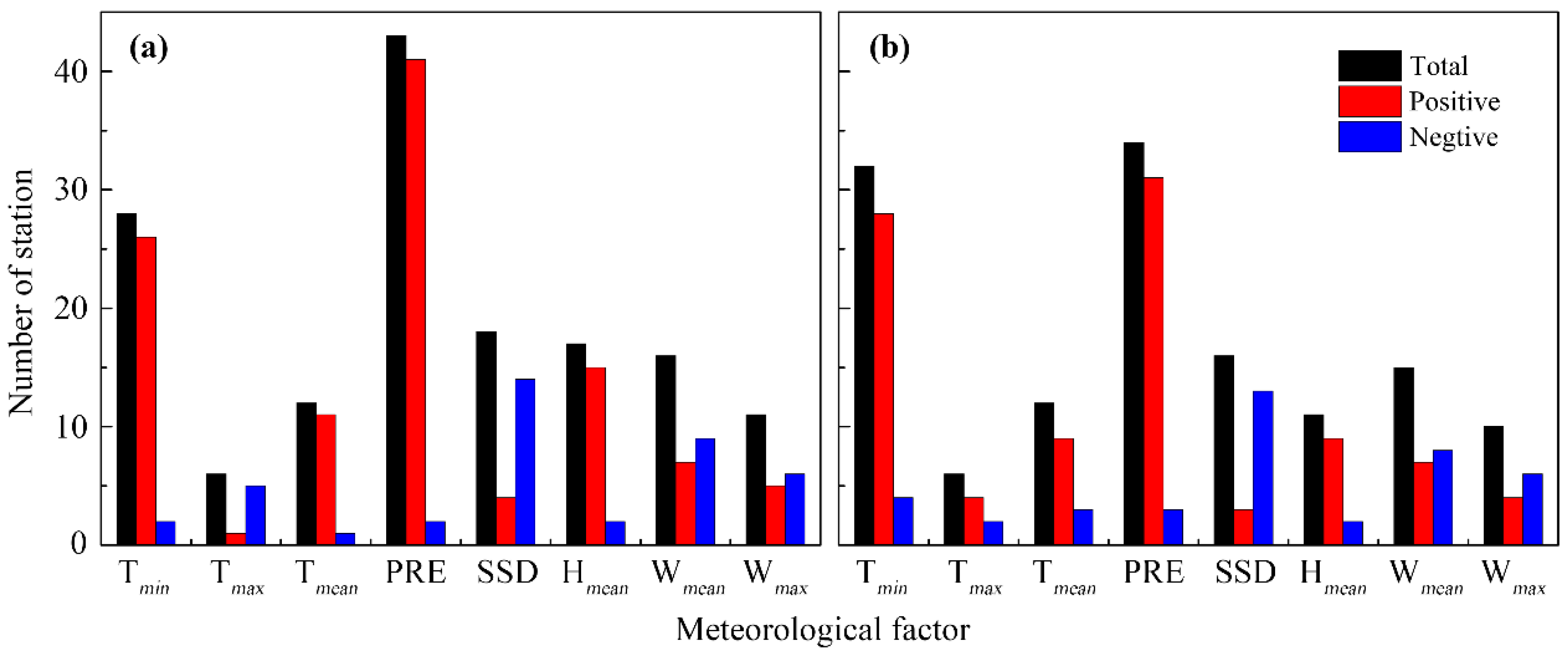
A stepwise linear regression model between NDVI/EVI2-retrieved MSD and climatic variables during the optimum period was successfully built at 85 (93% of total for NDVI-retrieved MSD) and 82 (90% of total for EVI2-retrieved MSD) stations. Precipitation during the optimum period is the primary variable selected for both NDVI- (43 stations) and EVI2-retrieved (34 stations) MSD models (Figure 4). The response of MSD to precipitation is mainly positive, and ranges from 0.02 to 0.40 day/mm (Figure S2a), suggesting that more preseason precipitation delays the alpine grassland senescence date. The second predominant variable selected for NDVI- (28 stations) and EVI2-retrieved (32 stations) MSD models is the minimum temperature during the optimum period (Figure 4), in which the response of MSD to the minimum temperature is also mostly positive and between 1.55 and 9.31 day/°C (Figure S2b), suggesting a higher preseason minimum temperature delays the MSD. The sunshine duration was selected at 18 stations for NDVI-retrieved MSD and 16 stations for EVI2-retrieved MSD (Figure 4), and the regression coefficients are mainly negative (−0.43 to −0.04 day/h, Figure S2c). Although other climatic variables were selected at a few stations, their influences on MSD could not be ignored. The effects of the mean relative humidity (Figure S2d) and maximum/mean temperature are generally positive, while the effect of the mean/maximum wind speed is mainly negative (Figure 4).

3.3. Spatial Pattern of the Selected Climatic Variables

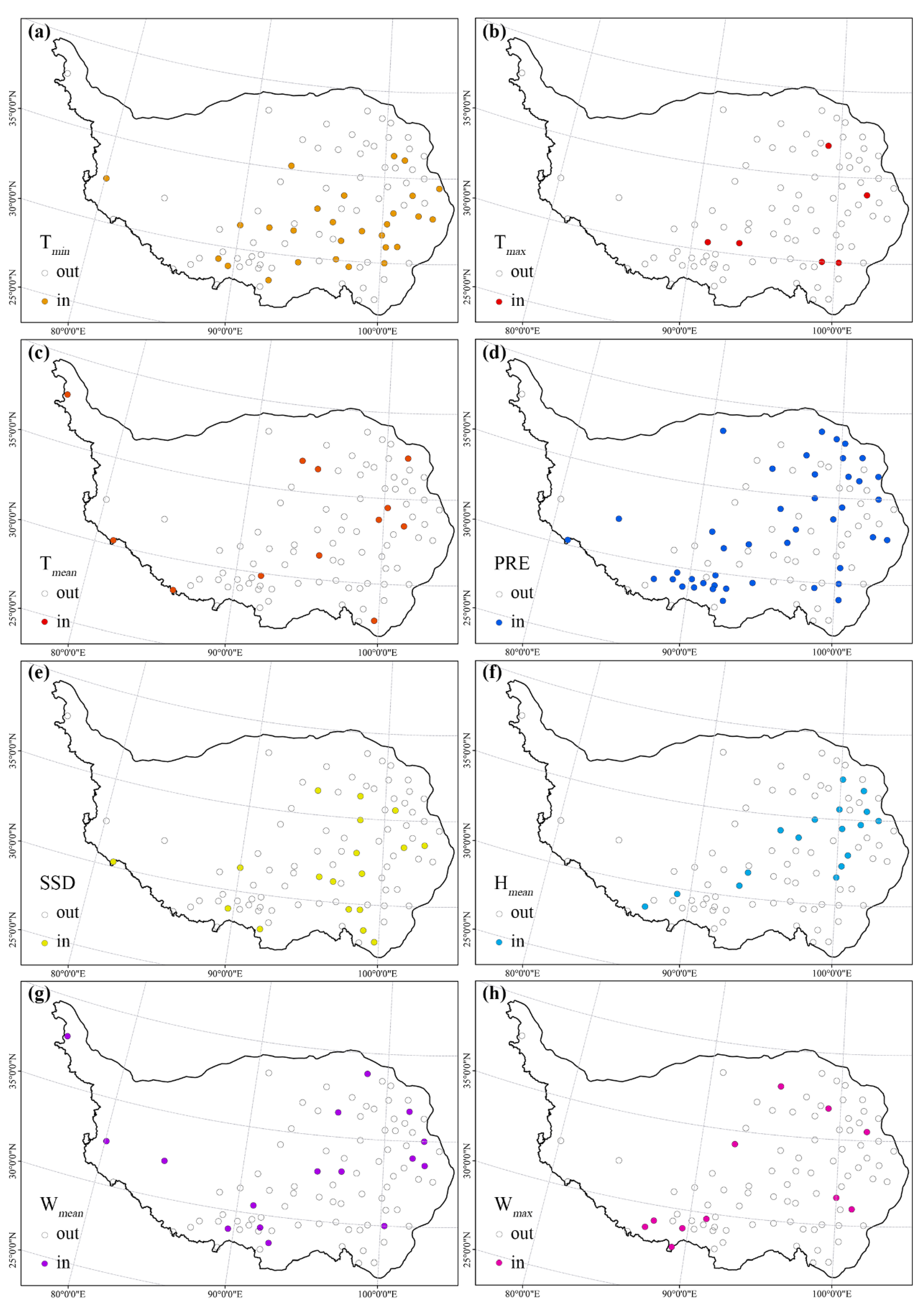
Figure 5 and Figure S3 show the spatial patterns of the stations with selected climatic variables using stepwise linear regression models for NDVI- and EVI2-retrieved MSD, respectively. The most extensively selected climate variable is precipitation and the corresponding stations are distributed mainly in the northeast and southwest parts of the QTP (Figure 5d and Figure S3d). The second extensively selected climate variable is the daily minimum temperature and the corresponding stations are in the eastern and southern parts of the QTP (Figure 5a and Figure S3a). The third extensively selected climate variable is the daily sunshine duration and the corresponding stations spread over the middle and southern sections of the QTP (Figure 5e and Figure S3e). The remaining climatic variables were selected at a few stations and their spatial patterns are generally discrete. It should be noted that more than one climatic variable was selected by the established models at 58% of the stations for NDVI-retrieved MSD and 51% of the stations for EVI2-retrieved MSD, respectively (Figure S4).

4. Discussion

By constructing stepwise linear regression models between MSD and climatic variables at satellite pixel windows around each of the 91 meteorological stations, we revealed the main controlling climatic factors of QTP alpine grassland autumn phenology. The result shows that precipitation, daily minimum temperature, and sunshine duration have the most extensive impacts on alpine grassland senescence. This is basically consistent with the results of previous studies, which found that preseason temperature, precipitation, and insolation are key climatic factors affecting temperate vegetation autumn phenology [7,8,19,20,38,39]. However, our research highlights that preseason precipitation is the most extensively controlling factor for interannual variations of alpine grassland senescence. This is different from the predominant temperature control on temperate woody plant autumn phenology [16,40,41]. It should be pointed out that there are significant differences between woody and herbaceous plants in responses to climatic factors. As herbs usually have shallower roots than woody plants, the precipitation response of autumn phenology in herbs should be more sensitive than woody plants, especially in arid and semiarid areas where precipitation is the main soil water source. The QTP climate is extremely cold and dry, and hydrothermal conditions are very harsh in most alpine grassland areas. However, the interannual variation of temperature is relatively stable, while precipitation varies greatly from year to year. Therefore, alpine grassland autumn phenology is likely more sensitive to precipitation variability than temperature fluctuation. That is, slight changes in precipitation in autumn could induce significant shifts in alpine grassland senescence dates. In this way, precipitation becomes the most important influencing factor of autumn phenology in alpine grassland. Regarding the role of preseason temperature, although some studies reported opposite effects of daily maximum and minimum temperatures on autumn phenology [11,23], our research confirmed that daily minimum temperature has stronger and more extensive influences on alpine grassland senescence rather than daily maximum temperature and daily mean temperature (Figure 4), which supports the process-based modelling of ground-observed herbaceous autumn phenology in the research region [26].
Stepwise linear regression models demonstrated that interannual variation of selected climatic factors affects the interannual variation of MSD at each station. The nature of the climatic factors’ effects can be characterized by regression coefficients. The response of MSD to precipitation during the optimum period is predominantly positive, which is consistent with previous studies [7,11,18,19,42]. Namely, more precipitation in autumn could improve the soil moisture and relieve the drought stress of alpine grassland [17], resulting in a delayed senescence. Similarly, the response of MSD to daily minimum temperature is also positive, because the minimum temperature may trigger leaf senescence by decreasing the light-saturated photosynthetic rate [43,44]. Thus, under moist and warm conditions in autumn, alpine grassland phenology would be delayed in most areas [9]. Different from the above two factors, the response of MSD to sunshine duration is mostly negative, namely, the longer the sunshine duration, the earlier the senescence. This is consistent with previous studies based on AVHRR GIMMS LAI data [7], but the mechanism is unclear. The response of MSD to the daily mean relative humidity is mostly positive, namely, higher air moisture may benefit the growth of alpine grassland and postpone senescence dates. Despite previous studies reporting a delaying effect of nighttime warming and an advancing effect of daytime warming on autumn QTP phenology [11,23], our study did not find a widespread negative response of MSD to the daily maximum temperature. As responses of MSD to the daily mean/maximum wind speed are uncertain, we could not identify the dominant response direction (positive or negative). Thus, wind speed might be just an ancillary climate factor influencing the senescence date of alpine grassland. Its functional mechanism might be more complex and needs further study. In addition, at 58% of the stations for NDVI-derived MSD and 51% of the stations for EVI2-derived MSD, multiple variables were selected by established stepwise regression models (Figure S4). This indicates that the combined effects of multiple climatic factors on autumn phenology are more significant than that of a single climatic factor at most stations. However, there is no discernible spatial aggregation of these stations and their spatial patterns are most likely random. Further studies should be carried out to reveal the mechanism of interaction effects of multiple climatic variables on QTP alpine grassland autumn phenology.
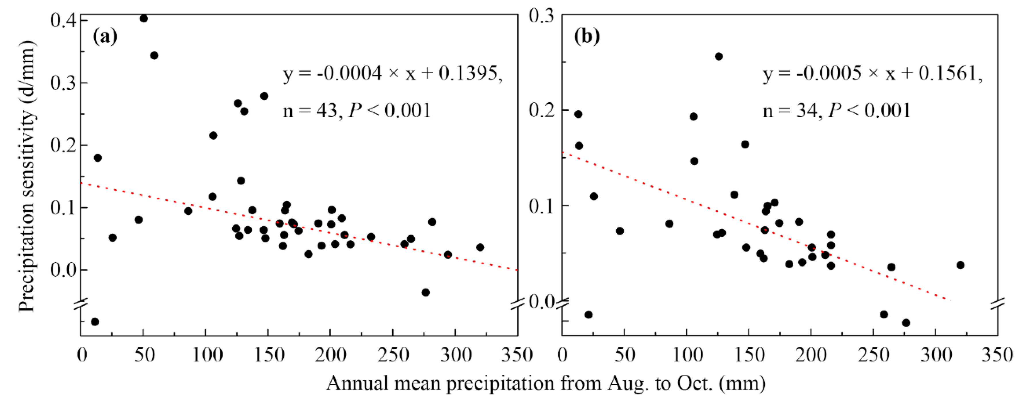
Although precipitation has the most extensive influence on interannual variation in alpine grassland autumn phenology, the spatial pattern of precipitation effects is not continuous (Figure 5d and Figure S3d) and the sensitivity of the autumn phenology response to preseason precipitation is also diverse (Figure S2a). In order to identify the spatial attribution of the sensitivity, we arranged regression coefficients in ascending order of the local autumn precipitation. The results show that the sensitivity of MSD to preseason precipitation is higher at stations with less autumn precipitation and lower at stations with more autumn precipitation (Figure 6). This implies that the control of preseason precipitation on autumn phenology is stronger at arid than at humid locations. Therefore, to more precisely predict QTP alpine grassland senescence dates under future climate change scenarios, precipitation effects should be added into existing process-based autumn phenology models coupling photoperiod and temperature [26].
Finally, it should be noted that the evaluation of satellite-derived phenology is always challenging because field-based observations are generally insufficient. In this study, we obtained the herb brown-off date for 13 years at 6 stations, which allowed us to properly evaluate the MSD derived from NDVI and EVI2 time series. Certainly, longer time series at more field stations could improve our understanding of MSD detections. Moreover, the six field stations (sites) are located at the northeastern QTP, which provided sufficient evaluation of MSD in this region. Of course, the MSD would be better evaluated if the field stations could be available across entire research areas.

5. Conclusions

Based on MODIS NDVI- and EVI2-retrieved land surface phenology data and stepwise linear regression models, we revealed the main climate drivers of QTP alpine grassland autumn phenology. Among the 91 stations, unitary and multiple regression models were successfully established at 93% of the stations for NDVI-retrieved MSD and 90% of the stations for EVI2-retrieved MSD. Preseason precipitation in autumn is the most extensive controlling factor affecting the interannual variation of the middle senescence date. On average, a 10 mm increase in autumn precipitation during the optimum length period may lead to a delay of 0.2 to 4 days in the middle senescence date (P < 0.05) across the alpine grasslands. The daily minimum air temperature is the second extensive controlling factor, namely, a 1 °C increase in the mean autumn minimum temperature during the optimum length period may induce a delay of 1.6 to 9.3 days in the middle senescence date (P < 0.05) across the alpine grasslands. Sunshine duration is the third extensive controlling factor and has a negative impact on the middle senescence date (−0.46 to −0.03 day/h). Moreover, relative humidity has a positive impact on the middle senescence date at a few stations, but wind speed effects are more uncertain than other factors. Further analysis indicates that the middle senescence date at stations with less autumn precipitation is more sensitive to precipitation variation than at stations with more autumn precipitation. This implies that autumn drought in arid regions would intensely accelerate alpine grassland leaf senescence. This study suggests that precipitation effects should be considered for improving process-based autumn phenology models in QTP alpine grasslands.

Supplementary Materials

The following are available online at https://www.mdpi.com/2072-4292/12/3/431/s1, Table S1: Geographical coordinates and elevation of phenological stations and observed plant species at each station; Figure S1: MAE (a)/(d), RMSE (b)/(e) and correlation coefficient (c)/(f) between multi-species mean brown-off date and NDVI/EVI2 retrieved median middle senescence date within different window size from 2000 to 2012; Figure S2: Frequency of stations with positive or negative regression coefficients between (a) precipitation (PRE)/(b) daily minimum temperature (Tmin)/(c) daily sunshine duration (SSD)/(d) daily mean relative humidity (Hmean) and the middle senescence date; Figure S3: Spatial patterns of stations with different climatic variables selected by the stepwise linear regression models for EVI2 retrieved MSD on the QTP. All legends are the same as in Figure 5; Figure S4: Number of climatic factors selected by the stepwise linear regression model in each meteorological station. (a) NDVI retrieved MSD, (b) EVI2 retrieved MSD.

Author Contributions

All authors made great contributions to the work. Specific contributions include research design (S.A., X.Q.C.), data collection and image processing (S.A., X.Y.Z.), data analysis (S.A.), and manuscript preparation (S.A., X.Q.C., X.Y.Z., W.G.L., S.L.R., L.X.). All authors have read and agreed to the published version of the manuscript.

Funding

This work was funded by the Premium Funding Project for Academic Human Resources Development in Beijing Union University no. BPHR2019DZ01 and the National Natural Science Foundation of China under grant nos. 41771049 and 41471033.

Acknowledgments

We thank the Meteorological Information Center of the China Meteorological Administration for providing phenological and climate data. We also thank NASA for providing free and ready access to the MODIS data and the writing improvement by Professor Mark D. Schwartz.

Conflicts of Interest

The authors declare no conflict of interest.

References

  1. Chen, H.; Zhu, Q.; Peng, C.; Wu, N.; Wang, Y.; Fang, X.; Gao, Y.; Zhu, D.; Yang, G.; Tian, J.; et al. The impacts of climate change and human activities on biogeochemical cycles on the Qinghai-Tibetan Plateau. Glob. Chang. Biol. 2013, 19, 2940–2955. [Google Scholar] [CrossRef] [PubMed]
  2. Zhang, G.; Zhang, Y.; Dong, J.; Xiao, X. Green-up dates in the Tibetan Plateau have continuously advanced from 1982 to 2011. Proc. Natl. Acad. Sci. USA 2013, 110, 4309–4314. [Google Scholar] [CrossRef] [PubMed] [Green Version]
  3. Zheng, Z.; Zhu, W.; Chen, G.; Jiang, N.; Fan, D.; Zhang, D. Continuous but diverse advancement of spring-summer phenology in response to climate warming across the Qinghai-Tibetan Plateau. Agr. Forest. Meteorol. 2016, 223, 194–202. [Google Scholar] [CrossRef]
  4. Yang, B.; He, M.; Shishov, V.; Tychkov, I.; Vaganov, E.; Rossi, S.; Ljungqvist, F.C.; Bräuning, A.; Grießinger, J. New perspective on spring vegetation phenology and global climate change based on Tibetan Plateau tree-ring data. Proc. Natl. Acad. Sci. USA 2017, 114, 6966–6971. [Google Scholar] [CrossRef] [Green Version]
  5. Chen, X.; An, S.; Inouye, D.W.; Schwartz, M.D. Temperature and snowfall trigger alpine vegetation green-up on the world's roof. Glob. Chang. Biol. 2015, 21, 3635–3646. [Google Scholar] [CrossRef]
  6. Ding, M.; Zhang, Y.; Sun, X.; Liu, L.; Wang, Z.; Bai, W. Spatiotemporal variation in alpine grassland phenology in the Qinghai-Tibetan Plateau from 1999 to 2009. Chin. Sci. Bull. 2012, 58, 396–405. [Google Scholar] [CrossRef] [Green Version]
  7. Che, M.; Chen, B.; Innes, J.L.; Wang, G.; Dou, X.; Zhou, T.; Zhang, H.; Yan, J.; Xu, G.; Zhao, H. Spatial and temporal variations in the end date of the vegetation growing season throughout the Qinghai–Tibetan Plateau from 1982 to 2011. Agr. Forest. Meteorol. 2014, 189–190, 81–90. [Google Scholar] [CrossRef]
  8. Cong, N.; Shen, M.; Piao, S. Spatial variations in responses of vegetation autumn phenology to climate change on the Tibetan Plateau. J. Plant. Ecol. 2016. [Google Scholar] [CrossRef] [Green Version]
  9. Zu, J.; Zhang, Y.; Huang, K.; Liu, Y.; Chen, N.; Cong, N. Biological and climate factors co-regulated spatial-temporal dynamics of vegetation autumn phenology on the Tibetan Plateau. Int. J. Appl. Earth Obs. 2018, 69, 198–205. [Google Scholar] [CrossRef]
  10. Meng, F.; Tsechoe, D.; Cui, S.; Wang, Q.; Li, B.; Wang, S. Changes of plant phenophases and their effects on the Qinghai-Tibetan Plateau. Chin. J. Nat. 2017, 39, 183–190. [Google Scholar] [CrossRef]
  11. Yang, Z.; Shen, M.; Jia, S.; Guo, L.; Yang, W.; Wang, C.; Chen, X.; Chen, J. Asymmetric responses of the end of growing season to daily maximum and minimum temperatures on the Tibetan Plateau. J. Geophys. Res.-Atmos. 2017, 122, 13,278–13,287. [Google Scholar] [CrossRef]
  12. Richardson, A.D.; Keenan, T.F.; Migliavacca, M.; Ryu, Y.; Sonnentag, O.; Toomey, M. Climate change, phenology, and phenological control of vegetation feedbacks to the climate system. Agr. Forest. Meteorol. 2013, 169, 156–173. [Google Scholar] [CrossRef]
  13. Gallinat, A.S.; Primack, R.B.; Wagner, D.L. Autumn, the neglected season in climate change research. Trends Ecol. Evol. 2015, 30, 169–176. [Google Scholar] [CrossRef] [PubMed]
  14. Piao, S.; Liu, Q.; Chen, A.; Janssens, I.A.; Fu, Y.; Dai, J.; Liu, L.; Lian, X.; Shen, M.; Zhu, X. Plant phenology and global climate change: Current progresses and challenges. Glob. Chang. Biol. 2019, 25, 1922–1940. [Google Scholar] [CrossRef] [PubMed]
  15. Ge, Q.; Wang, H.; Rutishauser, T.; Dai, J. Phenological response to climate change in China: A meta-analysis. Glob. Chang. Biol. 2015, 21, 265–274. [Google Scholar] [CrossRef] [PubMed]
  16. Fu, Y.H.; Piao, S.; Delpierre, N.; Hao, F.; Hanninen, H.; Liu, Y.; Sun, W.; Janssens, I.A.; Campioli, M. Larger temperature response of autumn leaf senescence than spring leaf-out phenology. Glob. Chang. Biol. 2018, 24, 2159–2168. [Google Scholar] [CrossRef] [PubMed]
  17. Shefferson, R.P.; Kull, T.; Hutchings, M.J.; Selosse, M.A.; Jacquemyn, H.; Kellett, K.M.; Menges, E.S.; Primack, R.B.; Tuomi, J.; Alahuhta, K.; et al. Drivers of vegetative dormancy across herbaceous perennial plant species. Ecol. Lett. 2018, 21, 724–733. [Google Scholar] [CrossRef] [Green Version]
  18. Liu, Q.; Fu, Y.S.H.; Zhu, Z.C.; Liu, Y.W.; Liu, Z.; Huang, M.T.; Janssens, I.A.; Piao, S.L. Delayed autumn phenology in the Northern Hemisphere is related to change in both climate and spring phenology. Glob. Chang. Biol. 2016, 22, 3702–3711. [Google Scholar] [CrossRef]
  19. Li, P.; Peng, C.; Wang, M.; Luo, Y.; Li, M.; Zhang, K.; Zhang, D.; Zhu, Q. Dynamics of vegetation autumn phenology and its response to multiple environmental factors from 1982 to 2012 on Qinghai-Tibetan Plateau in China. Sci. Total Environ. 2018, 637–638, 855–864. [Google Scholar] [CrossRef]
  20. Ding, M.; Chen, Q.; Li, L.; Zhang, Y.; Wang, Z.; Liu, L.; Sun, X. Temperature dependence of variations in the end of the growing season from 1982 to 2012 on the Qinghai–Tibetan Plateau. GISci. Remote Sens. 2015, 53, 147–163. [Google Scholar] [CrossRef]
  21. Zhu, W.; Jiang, N.; Chen, G.; Zhang, D.; Zheng, Z.; Fan, D. Divergent shifts and responses of plant autumn phenology to climate change on the Qinghai-Tibetan Plateau. Agr. Forest. Meteorol. 2017, 239, 166–175. [Google Scholar] [CrossRef]
  22. Zhang, Q.; Kong, D.; Shi, P.; Singh, V.P.; Sun, P. Vegetation phenology on the Qinghai-Tibetan Plateau and its response to climate change (1982–2013). Agr. Forest. Meteorol. 2018, 248, 408–417. [Google Scholar] [CrossRef]
  23. Wu, C.; Wang, X.; Wang, H.; Ciais, P.; Peñuelas, J.; Myneni, R.B.; Desai, A.R.; Gough, C.M.; Gonsamo, A.; Black, A.T.; et al. Contrasting responses of autumn-leaf senescence to daytime and night-time warming. Nat. Clim. Chang. 2018, 8, 1092–1096. [Google Scholar] [CrossRef] [Green Version]
  24. Editorial Board of Vegetation Map of China CAS. 1:1000,000 Vegetation Atlas of China; Hou, X., Ed.; Science Press: Beijing, China, 2001. [Google Scholar]
  25. China Meteorological Administration. Observation Criterion of Agricultural Meteorology; China Meteorological Press: Beijing, China, 1993. [Google Scholar]
  26. Lang, W.; Chen, X.; Qian, S.; Liu, G.; Piao, S. A new process-based model for predicting autumn phenology: How is leaf senescence controlled by photoperiod and temperature coupling? Agr. Forest. Meteorol. 2019, 268, 124–135. [Google Scholar] [CrossRef]
  27. Schaaf, C.; Wang, Z. MCD43A4 MODIS/Terra+Aqua BRDF/Albedo Nadir BRDF Adjusted Ref Daily L3 Global—500m V006 [Data set]; NASA EOSDIS Land Processes DAAC, 2015; Available online: https://doi.org/10.5067/MODIS/MCD43A4.006 (accessed on 17 January 2020).
  28. Schaaf, C.; Wang, Z. MCD43A2 MODIS/Terra+Aqua BRDF/Albedo Quality Daily L3 Global—500m V006 [Data set]; NASA EOSDIS Land Processes DAAC, 2015; Available online: https://doi.org/10.5067/MODIS/MCD43A2.006 (accessed on 17 January 2020).
  29. Zhang, X.; Jayavelu, S.; Liu, L.; Friedl, M.A.; Henebry, G.M.; Liu, Y.; Schaaf, C.B.; Richardson, A.D.; Gray, J. Evaluation of land surface phenology from VIIRS data using time series of PhenoCam imagery. Agr. Forest. Meteorol. 2018, 256–257, 137–149. [Google Scholar] [CrossRef]
  30. Huang, X.; Xiao, J.; Ma, M. Evaluating the performance of satellite-derived vegetation indices for estimating gross primary productivity using FLUXNET observations across the globe. Remote Sens. 2019, 11, 1823. [Google Scholar] [CrossRef] [Green Version]
  31. Zhang, X.; Friedl, M.A.; Schaaf, C.B. Global vegetation phenology from Moderate Resolution Imaging Spectroradiometer (MODIS): Evaluation of global patterns and comparison with in situ measurements. J. Geophys. Res. 2006, 111. [Google Scholar] [CrossRef]
  32. Zhang, X.; Friedl, M.A.; Schaaf, C.B.; Strahler, A.H.; Hodges, J.C.F.; Gao, F.; Reed, B.C.; Huete, A. Monitoring vegetation phenology using MODIS. Remote Sens. Environ. 2003, 84, 471–475. [Google Scholar] [CrossRef]
  33. Zhang, X. Reconstruction of a complete global time series of daily vegetation index trajectory from long-term AVHRR data. Remote Sens. Environ. 2015, 156, 457–472. [Google Scholar] [CrossRef]
  34. Zhang, X.; Liu, L.; Liu, Y.; Jayavelu, S.; Wang, J.; Moon, M.; Henebry, G.M.; Friedl, M.A.; Schaaf, C.B. Generation and evaluation of the VIIRS land surface phenology product. Remote Sens. Environ. 2018, 216, 212–229. [Google Scholar] [CrossRef]
  35. Chen, X.; Xu, L. Phenological responses of Ulmus pumila (Siberian Elm) to climate change in the temperate zone of China. Int. J. Biometeorol. 2012, 56, 695–706. [Google Scholar] [CrossRef] [PubMed]
  36. Kleinbaum, D.; Kupper, L.; Muller, K.; Nizam, A. Selecting the best regression equation. In Applied Regression Analysis and Other Multivariable Methods, 3rd ed.; China Machine Press: Beijing, China, 2003; pp. 398–399. [Google Scholar]
  37. Huang, C.; Townshend, J.R.G. A stepwise regression tree for nonlinear approximation: Applications to estimating subpixel land cover. Int. J. Remote Sens. 2010, 24, 75–90. [Google Scholar] [CrossRef]
  38. Liu, Q.; Fu, Y.H.; Zeng, Z.; Huang, M.; Li, X.; Piao, S. Temperature, precipitation, and insolation effects on autumn vegetation phenology in temperate China. Glob. Chang. Biol. 2016, 22, 644–655. [Google Scholar] [CrossRef] [PubMed]
  39. Yang, Y.T.; Guan, H.D.; Shen, M.G.; Liang, W.; Jiang, L. Changes in autumn vegetation dormancy onset date and the climate controls across temperate ecosystems in China from 1982 to 2010. Glob. Chang. Biol. 2015, 21, 652–665. [Google Scholar] [CrossRef] [PubMed]
  40. Liu, G.; Chen, X.; Zhang, Q.; Lang, W.; Delpierre, N. Antagonistic effects of growing season and autumn temperatures on the timing of leaf coloration in winter deciduous trees. Glob. Chang. Biol. 2018, 24, 3537–3545. [Google Scholar] [CrossRef]
  41. Delpierre, N.; Dufrêne, E.; Soudani, K.; Ulrich, E.; Cecchini, S.; Boé, J.; François, C. Modelling interannual and spatial variability of leaf senescence for three deciduous tree species in France. Agr. Forest. Meteorol. 2009, 149, 938–948. [Google Scholar] [CrossRef]
  42. Jiang, J.; Chen, L.; Ding, W.; Zhang, Y.; Wei, Y. Response of desert herbaceous plants to drought stress. Chin. Agric. Bull. 2017, 33, 68–73. (In Chinese) [Google Scholar]
  43. Zheng, Y.L.; Feng, Y.L.; Lei, Y.B.; Yang, C.Y. Different photosynthetic responses to night chilling among twelve populations of Jatropha curcas. Photosynthetica 2010, 47, 559–566. [Google Scholar] [CrossRef]
  44. Matos, F.S.; de Oliveria, L.R.; Galvão de Freitas, R.; Evaristo, A.B.; Missio, R.F.; Oliva Cano, M.A.; Antônio dos Santos Dias, L. Physiological characterization of leaf senescence of Jatropha curcas L. populations. Biomass Bioenerg. 2012, 45, 57–64. [Google Scholar] [CrossRef]
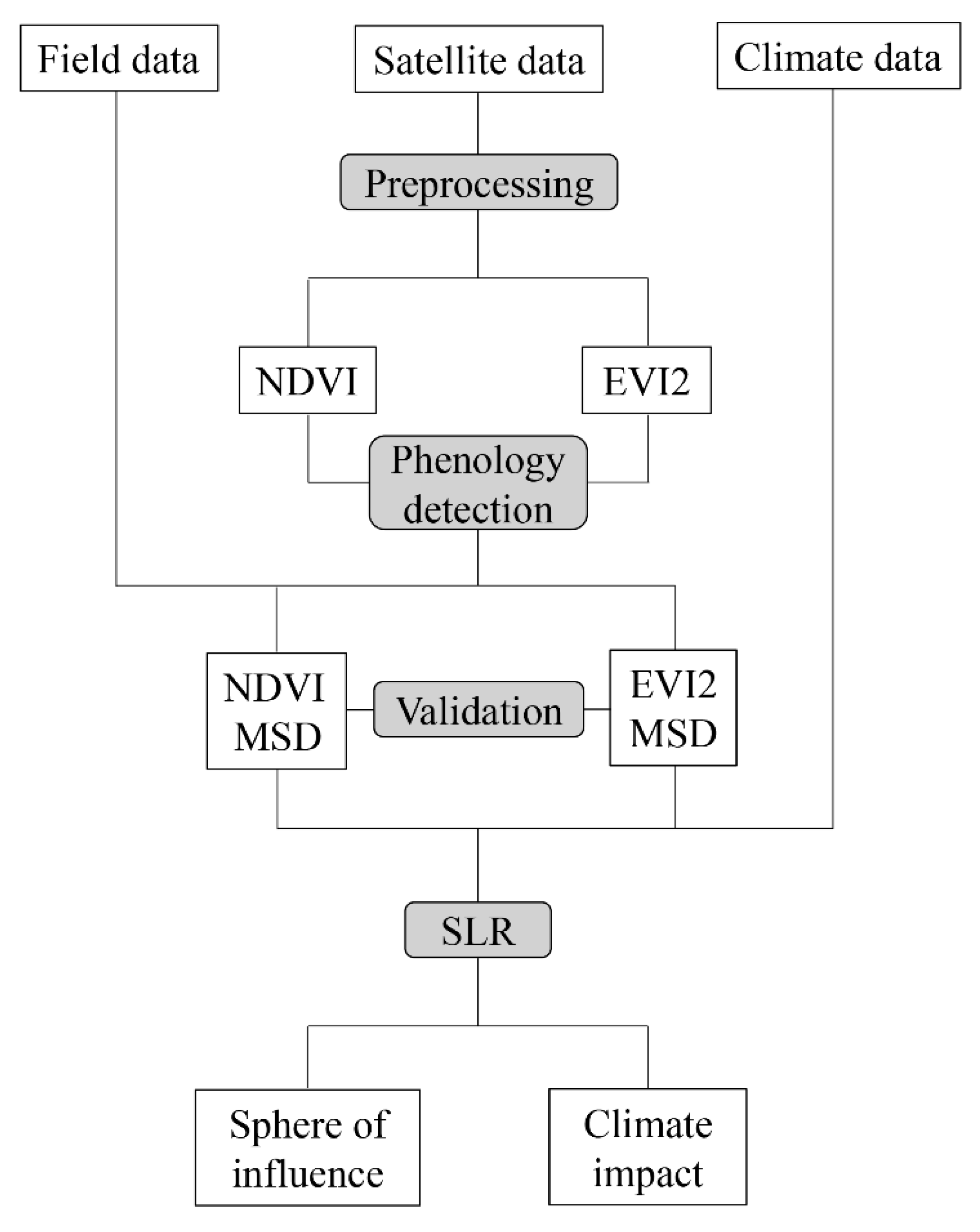
Figure 1. Flow diagram of data processing and analyses. MSD denotes the middle senescence date. SLR denotes the stepwise linear regression.
Remotesensing 12 00431 g001
Figure 2. Spatial distribution of major vegetation types and meteorological and phenological stations on the Qinghai-Tibet Plateau (QTP). The red dashed line denotes boundaries of climatic subdivisions [26]. A, B, C, and D represent humid, sub-humid, semi-arid, and arid regions, respectively.
Remotesensing 12 00431 g002
Figure 3. Moderate Resolution Imaging Spectroradiometer (MODIS) normalized difference vegetation index (NDVI) and 2-band enhanced vegetation index (EVI2) curve fitting and middle senescence date extraction. (a) A sample pixel in the steppe area and (b) a sample pixel in the meadow area. The black dot denotes the calculated middle senescence point of alpine grassland on the fitting curves and the corresponding horizontal axis coordinate is the middle senescence date (MSD).
Remotesensing 12 00431 g003
Figure 4. Number of stations and regression coefficient sign symbols for climatic variables selected by stepwise linear regression models for (a) NDVI- and (b) EVI2-retrieved MSD. Tmin, Tmax, Tmean, PRE, SSD, Hmean, Wmean, and Wmax denote the daily minimum, maximum, mean air temperature, accumulated precipitation, sunshine duration, mean relative humidity, mean, and maximum wind speed during the optimum length periods, respectively. The black bar is the total number of stations for the selected climate variables. The red and blue bar are the number of stations with positive and negative regression coefficients for the selected climate variables, respectively.
Remotesensing 12 00431 g004
Figure 5. Spatial patterns of stations with different climatic variables (a) Tmin (b) Tmax (c) Tmean (d) PRE (e) SSD (f) Hmean (g) Wmean (h) Wmax selected by the stepwise linear regression models for NDVI-retrieved MSD on the QTP. Tmin, Tmax, Tmean, PRE, SSD, Hmean, Wmean, and Wmax denote the same meanings as in Figure 4. Circles in different colors represent meteorological stations with different climatic variables. “Out” means that the climate variable was not selected by the stepwise linear regression model, while “in” means that the climate variable was selected.
Remotesensing 12 00431 g005
Figure 6. Regression analyses between annual mean precipitation from August to October and sensitivity of MSD to preseason precipitation at the 91 meteorological stations. (a) NDVI-derived MSD, (b) EVI2-derived MSD. The red dashed line is the Theil–Sen linear trend tested using the Mann–Kendall significance test.
Remotesensing 12 00431 g006