The MODIS Global Vegetation Fractional Cover Product 2001–2018: Characteristics of Vegetation Fractional Cover in Grasslands and Savanna Woodlands


1
CSIRO Land and Water, Black Mountain, ACT 2601, Australia
2
Department of Earth System Science and Policy, University of North Dakota, Grand Forks, ND 58202, USA
*
Author to whom correspondence should be addressed.
Remote Sens. 2020, 12(3), 406; https://doi.org/10.3390/rs12030406
Submission received: 24 December 2019
/
Revised: 10 January 2020
/
Accepted: 24 January 2020
/
Published: 28 January 2020
(This article belongs to the Special Issue Remote Sensing of Savannas and Woodlands)
Abstract
:Vegetation Fractional Cover (VFC) is an important global indicator of land cover change, land use practice and landscape, and ecosystem function. In this study, we present the Global Vegetation Fractional Cover Product (GVFCP) and explore the levels and trends in VFC across World Grassland Type (WGT) Ecoregions considering variation associated with Global Livestock Production Systems (GLPS). Long-term average levels and trends in fractional cover of photosynthetic vegetation (FPV), non-photosynthetic vegetation (FNPV), and bare soil (FBS) are mapped, and variation among GLPS types within WGT Divisions and Ecoregions is explored. Analysis also focused on the savanna-woodland WGT Formations. Many WGT Divisions showed wide variation in long-term average VFC and trends in VFC across GLPS types. Results showed large areas of many ecoregions experiencing significant positive and negative trends in VFC. East Africa, Patagonia, and the Mitchell Grasslands of Australia exhibited large areas of negative trends in FNPV and positive trends FBS. These trends may reflect interactions between extended drought, heavy livestock utilization, expanded agriculture, and other land use changes. Compared to previous studies, explicit measurement of FNPV revealed interesting additional information about vegetation cover and trends in many ecoregions. The Australian and Global products are available via the GEOGLAM RAPP (Group on Earth Observations Global Agricultural Monitoring Rangeland and Pasture Productivity) website, and the scientific community is encouraged to utilize the data and contribute to improved validation.
Keywords:
vegetation; grassland; savanna; fractional cover; trend; ecoregion; bare soil; livestock; production systems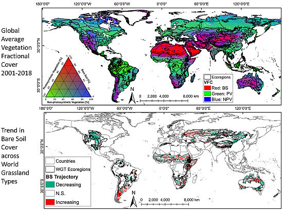
1. Introduction
Vegetation Fractional Cover (VFC) is an important global indicator of land cover change, land use practice, and landscape and ecosystem function [1,2]. Seasonal dynamics and long-term trends in the fractional cover of photosynthetic vegetation (FPV), non-photosynthetic vegetation (FNPV), and bare soil (FBS) may identify changes in cropping cycles, impacts of livestock grazing, clearing or planting of woody vegetation, and ecosystem responses to climate shifts. The Australian Vegetation Fractional Cover Product (AVFCP) is derived from the 500 m MODIS (MODerate Resolution Imaging Spectroradiometer) NBAR (Nadir BRDF-adjusted Reflectance) product (MCD43A4) and has been comprehensively documented, validated, and improved over several versions [3,4,5,6]. In this study, we present the Global Vegetation Fractional Cover Product (GVFCP) based on the same methodology. Both the Australian and Global products are available through the GEOGLAM RAPP (Group on Earth Observations Global Agricultural Monitoring Rangeland and Pasture Productivity) website (https://map.geo-rapp.org). A list of abbreviations appears in Table A1.
A key feature of the GVFCP is the explicit sensitivity to FNPV enabling better discrimination of dry cellulosic vegetation and bare soil fractions than is possible with the family of greenness indices. For this reason, the GVFCP is particularly important for monitoring of the non-forested and non-desert global biomes, woodlands, savannas, grassland and shrublands, where the overstory canopy is open, and understory dynamics involve the relationships between cellulosic herbaceous vegetation and/or senescent arboreal leaf litter and bare soil. The first version of the AVFCP [3] used the relationship between the Normalised Difference Vegetation Index (NDVI) and the Short Wave Infrared Ratio (SWIR32; a ratio of the MODIS 2130 nm and MODIS 1640 nm bands) in a linear unmixing method to approximate the relationship between NDVI and the Cellulose Absorption Index (CAI) developed and demonstrated by [7,8,9,10,11]. An improved version of the AVFCP utilizes all seven MODIS NBAR bands plus band transformations and interaction terms in a sophisticated unmixing algorithm [4]. Recent recalibration of the AVFCP with MODIS Collection 6 inputs and an updated validation data set established improvements in the accuracy of the retrieved fractions of photosynthetic vegetation (FPV RMSE 0.112), non-photosynthetic vegetation (FNPV RMSE 0.162), and bare soil (FBS RMSE 0.130) [5].
Based on Australian studies [12,13,14], the AVFCP provides a consistent and verifiable estimate of the cover fractions for green canopy, senescent vegetation and surface litter, and the visible soil surface. Given the diversity of natural ecosystems across Australia that include tropical rainforest, tropical and temperate savanna, temperate grasslands, semi-arid and arid shrublands and grasslands, temperate eucalypt forests, and temperate rainforest, and the extent of agricultural and pastoral lands across Australia, it is reasonable to propose that the GVFCP should perform with similar levels of uncertainty across the diversity of global land covers and land uses, especially in the non-forested and non-desert biomes.
Many global analyses have focused on tree cover change [15,16,17] and land cover change [18]. The recent comprehensive study of [19] partitions cover into tall vegetation, short vegetation, and bare soil, and the greening analysis of [20] looks at trends in the annual values of the MODIS leaf area index product [21]. In addition, other studies have focused on the total cover and soil or bare fractions [22,23]. There are several global tree cover [24,25] and tree cover change [15] products at multiple resolutions and many FAPAR (Fraction of Absorbed Photosynthetically Active Radiation) [26,27] and green canopy cover or leaf area index products [28,29,30]. The global cover change study by [19] identifies changes in short vegetation (which includes shrubs under 5 m in height) and bare ground. The cover fractions are mapped from peak growing season canopy [19] meaning that deciduous savanna trees and shrubs are probably fully foliated, and understory grasses are actively growing. By contrast, the GVFCP at full temporal and spatial resolution follows the phenology of overstory and understory throughout the seasons and explicitly retrieves FNPV representing senescent understory.
Studies focusing on global scale cover, dynamics, and change in savanna landscapes are less common (e.g., [31,32]), but a study based on persistence of GIMMS (Global Inventory Modeling and Mapping Studies) NDVI signals indicated larger areas of increased than decreased vegetation persistence [33]. However, there has been considerable discussion on the nature of stable states, methods of detection, and drivers of change in savannas (e.g., [34,35,36,37]). Due to the specific methodology used to derive it, the GVFCP provides a unique measure of global changes in vegetation fractional cover especially important for woodlands, savannas, grasslands and shrublands which are subject to heavy utilization and conversion for human food production and where cellulosic herbaceous cover is important.
It is instructive to provide context for the behaviour of remote sensing products using global datasets that are wholly or partially independent of remote sensing, and describe global vegetation in terms relevant to conservation, ecosystem function, and productivity. The Terrestrial Ecoregions of the World (TEoW; [38]) and the subset of these used to define World Grassland Types (WGT [39]) provides an effective framework within which to view the patterns of VFC for the grassy ecoregions of the world. Since these grassy ecoregions are subject to major utilization by humans for extensive and intensive agriculture, the Global Livestock Production Systems (GLPS) classification [40] provides a means to sample variation within WGT Ecoregions due to differences in utilisation between production systems.
In this study we have three objectives:
- (1)
- To present the GVFCP (using a resampled 5 km2 resolution version) and illustrate the long-term global geographical patterns of FPV, FNPV, and FBS using the TEoW [38].
- (2)
- (3)
- To examine the levels and trends in FPV, FNPV, and FB in savanna, woodland and scrub grassland (SWSG) Ecoregions of the WGT and explore VFC trajectories in selected example ecoregions where major changes are occurring.
2. Materials and Methods
The analysis undertaken here provides an overview of global VFC in map form; records benchmark average levels of VFC across production systems for Formation, Division, and Ecoregion areas of the grassy biomes of the world; and documents long-term trends in VFC from 2001–2018 for these areas. The analysis is designed to provide an overview framework and baseline for more detailed future studies.
2.1. Data
2.1.1. Global Vegetation Fractional Cover Product
The GVFCP estimates the fractions of photosynthetic (green) vegetation (PV), non-photosynthetic (non-green) vegetation (NPV), and bare soil (BS) within the pixel using a spectral linear unmixing method [4,5]. The base version of the GVFCP, available on the GEOGLAM RAPP-MAPP website (https://map.geo-rapp.org) is calculated using reflectance values from the MODIS MCD43A4 product which is a rolling daily 16-day composite weighted to retrieve the value on the ninth day of the 16-day period [41]. The GVFCP utilizes every eighth day from the MCD43A4 product starting with day one of each year with an adjustment for leap years proving 46 dates in each calendar year. The data are stored in a geographic latitude-longitude raster with a WGS84 spheroid. A second monthly composite product (also available on the website) is created by aggregating all values falling within each calendar month using a medoid function (a multidimensional median) following [42]. Pixels flagged as water, snow, or low quality in the MCD43A4 product are ignored in the calculation of the GVFCP. The current product is the result of a decade of development and the most recent version derived from MODIS Collection 6 NBAR data was calculated and validated using an updated and expanded database of 3022 ground measurements of fractional cover across Australia [5] and had a Root Mean Square Error (RMSE) of 11.3%, 16.1%, and 14.7% in the PV, NPV, and BS fractions, respectively. The GVFCP is derived from spectral unmixing of all seven MODIS optical bands from the 500 m MODIS Nadir BRDF-adjusted Reflectance Product (NBAR, MCD43A4 Collection 6; see Appendix A Table A1 for abbreviations) using previously described methods [4]. The product consists of four derived layers corresponding to the decimal values of cover fractions FPV, FNPV, FBS, and the residual from the spectral unmixing in reflectance values (RNORM). The GVFCP is calculated from the daily NBAR data product producing a phased 16-day composite every eight days. For this overview study, the monthly version of the product was used and resampled to 0.05° resolution (approximately 5 km2) by averaging.
2.1.2. Terrestrial Ecoregions of the World
The Terrestrial Ecoregions of the World (TEoW) provide a biogeographic realization of terrestrial biodiversity [38] (Figure 1a). They represent land areas that share species, ecosystems, seasonal dynamics, and environmental conditions, and therefore, in part, indicate boundaries for intrinsic capability or risk for human uses. This dataset is used to meet the first objective of this study by providing general context for the description of the GVFCP at TEoW Realm level. Since an important attribute of the GVFCP is the derivation of FNPV and FBS, additional datasets that focus on the characteristics and human utilization of the subset of ecoregions either partially or totally dominated by herbaceous vegetation were employed to examine behaviour in the grassy regions of the world.
2.1.3. World Grassland Types
The World Grassland Types (WGT; [39]) represent a subset of terrestrial ecoregions that were combined with the International Vegetation Classification (IVC; [43]) to spatially define the major grassy vegetation systems of the world (Figure 1b; see Table A1 for abbreviations). They describe 75% of the IVC grasslands using ecoregions. The remaining IVC grasslands were absent from the mapping due to their fine scale distribution [39]. The WGT Ecoregions cover an area of 35.5 M km2. The Tropical Lowland Shrubland, Grassland and Savannas (TLSGS), Tropical Montane Shrubland, Grassland and Savanna (TMSGS), and the Warm Semi-Desert Scrub and Grassland (WSDSG) WGT Formations were selected to represent the savanna, woodland and scrub grasslands (SWSG) which are the focus of this Special Issue. These SWSGs occupy 46.9% of the WGT area (16.7 M km2) of which 9.5 M km2 are in the northern hemisphere in Africa and neo-tropical South America, and 7.16 M km2 are in the southern hemisphere in Africa, Australia, and South America. The northern hemisphere contains 7.0 M km2 of TLSGS, 0.3 M km2 of TMSGS, and 2.2 M km2 of WSDSG. The southern hemisphere contains 6.1 M km2 of TLSGS, 0.25 M km2 of TMSGS, and 0.82 M km2 of WSDSG.
2.1.4. Global Livestock Production Systems
The Global Livestock Production Systems (GLPS) data describes the terrestrial land surface using livestock density maps, crop type maps, land cover, and information on management practices [40] (Figure 1c). The classification describes 12 production systems combining rangelands (L—grazing only), mixed rainfed and mixed irrigated production (M—grazing and cropping) with hyper-arid (Y), arid (A), humid (H), and temperate (T) environments at a spatial resolution of 0.00833° (approximately 1 km2; Figure 1c). These are: Rangelands Hyper-arid (LGY); Rangelands Arid (LGA); Rangelands Humid (LGH); Rangelands Temperate (LGT); Mixed Rainfed Hyper-arid (MRY); Mixed Rainfed Arid (MRA); Mixed Rainfed Humid (MRH); Mixed Rainfed Temperate (MRT); Mixed Irrigated Hyper-arid (MIY); Mixed Irrigated Arid (MIA); Mixed Irrigated Humid (MIH); and Mixed Irrigated Temperate (MIT). The remaining land areas are classified as Urban or Other (such as forest, ice, rock, etc.). These classes describe land use with each WGT Ecoregion. The WGT Ecoregions are dominated by seven GLPS types with the six major production systems being: LGA (36.8%); LGT (17.6%); MRA (8.4%); MRT (14.5%); LGH (4.7%); and MRH (5.6%) and the remaining area being Other.
2.2. Analysis Method
2.2.1. Trend Analysis for World Grassland Types
The long-term trend from 2001–2018 in the monthly FPV, FNPV, and FBS was evaluated for the WGT Ecoregions using the Mann–Kendall test [44,45] with a custom-built function in IDL. This non-parametric test detects monotonic trends in time series data where the least squares regression approach is invalid due the autocorrelation in time series data derived from remote sensing. We used the Mann–Kendall approach for trend analysis on the full monthly data set since these data provided more observations than annual means by a factor of 12. The time series was smoothed by the medoid procedure, spatially averaged from 500 m to 5 km pixels by the pixel aggregation, and completely continuous in the WGT Ecoregions. As a result, we did not consider it necessary to apply the seasonal Kendall method [46]. The significance (p-value) of the slope in each pixel was recorded. Global maps of pixels within the WGT Ecoregions where trends were significant at p < 0.1 were produced. The same spatial patterns and trends were evident at p < 0.05 but patterns were clearer and more contiguous at p < 0.1 similar to [20].
2.2.2. Summarizing Levels and Trends across World Grassland Types and Savanna-Woodlands
The levels and trends in VFC were examined at increasing levels of detail across the WGT. The WGT and GLPS layers were combined to create a composite layer with individual classes for each GLPS-ecoregion combination. Class mean and standard deviation values for long-term average and trend in FPV, FNPV, and FBS were extracted using ArcGIS® zonalstats. For trends, zonal statistics were collected only for slope values > 0.1 or < −0.1 using a mask that restricted extractions to only those pixels with significance at p < 0.1. The areas of significant trend by Division and Ecoregion were calculated on geographic grids using a weighted area algorithm to correct for pixel distortion with latitude away from the equator. The variation across GLPS types within WGT Divisions was displayed using the fence box plot. The fence box analysis plots the median and divides the observed values into quartiles with first and third quartiles defining the hinges, and the upper and lower fences being defined by multiplying the interquartile range by 1.5. The whiskers represent the minimum and maximum observations falling inside the fences and points falling outside this range represent outliers. The fence-box plots at Division level therefore show the range in mean values among GLPS types within that Division (whether it contains one or many Ecoregions) and the range in the standard deviation values from each GLPS type within that Division. Examination of the SWSG was carried out by the same methods at individual ecoregion level, and GLPS class behaviour was explored within selected ecoregions exhibiting large areas of significant trends.
3. Results
3.1. Global Patterns of Average VFC
Global geographical distribution of long-term average FPV and FBS exhibit the typical associations with forests and deserts and the gradients in between (Figure 2). The distribution of long-term average FNPV tends to highlight the large grasslands of North America, South America, central Eurasia, Tibet, Mongolia, and the savannas of southern Africa and Australia (Figure 2). Based on TEoW definitions, there are 19.5 M km2 of tropical and subtropical grasslands, shrubland, and savannas representing 13.26% of the terrestrial land surface (Table 1). In addition, the global coverage of Temperate Grasslands and Shrublands, Montane Grasslands and Shrublands, and Flooded Grassland and Savannas brings the total area of grassy biomes to 35.439 M km2 representing 24.05% of the terrestrial land surface. Across these grassy biomes, the Montane Grasslands and Shrublands have lower average FPV and higher average FBS than the other grassy biomes (Table 1). Temperate and Montane Grasslands and Shrublands have higher average FNPV than the Tropical and Subtropical Grasslands, Savannas and Shrublands and the Flooded Grassland and Savannas. The global latitudinal variation in average FPV, FNPV, and FBS exhibits typical peaks in FPV for tropical forests between 20° S and 20° N and boreal forests above 50° N and in FBS in northern and southern hemisphere arid lands between latitudes 20 and 30° (Figure 3). However, there is a notable rise in FNPV between 20 and 40° N which may reflect the large expanses of steppe environments either limited by precipitation or converted to cereal cropping. With much less land at mid- to low-latitudes, the dynamics between the cover fractions in the southern hemisphere exhibit distinct narrow latitude zones of oscillation between higher and lower levels of FPV and FNPV between 30 and 45°.
3.2. Variation in Vegetation Fractional Cover within Global Livestock Production Systems
The GLPS types exhibit wide variation in mean FPV across ecoregions with large ranges between upper and lower hinges and fences. There was less variation in mean FNPV and FBS, although the latter exhibited wide variation in the upper and lower fence values and more extreme (outlier) ecoregions than FPV and FNPV (Figure 4). Median and hinge values for FPV increase from hyper-arid (Y) to arid (A) to humid (H) for both grazing (L) and mixed (M) land uses, while median and hinge values for temperate (T) systems were similar to arid systems for grazing and mixed land uses. The average FBS also exhibits a wide range of values across ecoregions within a GLPS type with values > 70% and ≤ 5% for LGA and LGT suggesting differences in interactions between the vegetation and livestock type and management. Average FBS is notably low across ecoregions for both LGH and MRH. Average FNPV exhibits a lower range across ecoregions within a GLPS type, and between GLPS types than FPV, with median values of ecoregion means across all GLPS types lying between 25%–45%. A gross indication of the impact of the GLPS on vegetation cover can be gained from comparing the medians and ranges of the Other class with those of the production systems. For FPV, the median value is higher and the range is wider than all GLPS types except for the LGH, MRH, and MIH types where tropical pasture and cropland conversion results in higher productivity. Similarly, FBS for the Other class is lower than all GLPS types except for the LGH, MRH, and MIH types.
3.3. Variation in Average Vegetation Fractional Cover in World Grassland Type Divisions
The WGT Ecoregions are organized by Formations and Divisions (Table A2) with the Formations representing a broad structural type, and the Divisions representing the regional geographical representations of these Formations. The WGT Divisions exhibit a wide range of long-term average levels of FPV, FNPV, and FBS and substantial variation in the levels of the upper and lower hinges and fences (Figure 5) There is also major variation in the standard deviations of VFC among GLPS classes with a WGT Division. Across the WGT, FPV exhibits greater variation in upper and lower hinge values than FNPV and FBS. The Divisions within the TLSGS and TMSGS Formations (lowland and montane savanna woodlands) exhibit relatively high average FPV and low average FBS except for the NSSDSG Division which covers the Sahelian region of northern Africa. Among the other Divisions, the MBDG, MSACSDSG, PCSDSG, TACSDSG, and AWSDSG within the CSDSG (semi-desert) and MSGFM (Mediterranean) Formations are notable for very low average FPV, median levels of FNPV close to 50%, and relatively high levels of FBS. The WEGS Division in western Eurasia, and the montane AMGS, and the alpine CAASFMG Divisions exhibit wide variation in average FPV but WEGS exhibits a lower median and much lower range between hinge values for standard deviation than AMGS and CAASFMG.
3.4. Trends in Vegetation Fractional Cover
3.4.1. World Grassland Types
The spatial distribution of pixels exhibiting significant trends at p < 0.1 is shown in Figure 6. Across the WGT Ecoregions, the extent of significant trends was greater for FBS than for the vegetation fractions since vegetation cover trends were split between change in FPV and change in FNPV and these vary in different ways for different geographies. There are significant positive and negative long-term trends in FPV, FNPV, and across the WGT Ecoregions (Figure 7). The WGT Ecoregions are displayed over the global map of countries, showing that the significant trends affect many African and Eurasian countries whilst the USA, Brazil, Argentina, and Australia with their large areas of grassland and savanna experience change over very large areas. There are positive trends in FPV in the northern great plains of North America, parts of China, and parts of eastern and southern Africa (Figure 7a). There are notable negative trends in FNPV in Patagonia, across Sahelian and Sudanian Africa, in Mongolia and on the Tibetan Plateau, and in the Mitchell Grasslands of Northern Australia (Figure 7b). However, the largest areas of significant trends occur for FBS with negative trends across the Great Plains of North America, across central China, across northern and southern Australia, and areas of positive trends in Sahelian, Sudanian and East Africa, western Mongolia, Ukraine and southern Russia, and the Mitchell Grasslands of Northern Australia (Figure 7c).
Examination of the variation due to GLPS in trends for WGT Divisions show that although the median values within Divisions seldom exceed ± 0.2%, the lower hinge values are as low as −0.5% and the upper hinge values are as high as 0.4% for FPV, as low as −0.4%, as high as 0.4% for FNPV, and as high as 0.4% for FBS and as low as −0.5% for FBS (Figure 8). It is particularly notable that certain Divisions (CAASMG, EECSDSG, WECSDSG, EEGS, NAGS, and WEGS) contain individual GLPS-Ecoregion combinations with positive and negative trends in FNPV as great as ± 0.5% and in FBS as low as −1.0% and as high as 0.5% that sit well beyond the upper and lower fences (outliers). These Divisions are in the northern hemisphere and are in the alpine ASFMG, semi-desert CSDSG, Mediterranean MSGFM, and temperate TGMS Formations suggesting major land use effects between GLPS types. Among the Divisions in the TLSGS and TMSGS Formations (savanna woodlands), most northern hemisphere Divisions show small increasing trends in FPV and relatively insignificant changes in FNPV and FBS. However, in the southern hemisphere the lower hinge and fence values for FPV, upper and lower hinge and fence values for FNPV, and upper hinge and fence values for FBS in the mopane and bushveld savannas (MS), and the montane WCAMWS, AMGS, and BPMSG identify GLPS classes with negative trends in FPV and positive trends in FNPV and FBS (Figure 8).
The fence box analysis describes the range in variation in VFC trends across GLPS types within WGT Divisions, however the Divisions vary in size and this may mask localised strong trends in large Divisions (such as the Sahelian Acacia Savanna which is a single enormous Ecoregion) and emphasize trends in small Divisions with more uniform climate, terrain, and edaphic features (such as the Ethiopian Montane Grasslands and Woodlands). Hence, it is important to define the area and area percentages where significant positive and negative trends in VFC are occurring (Figure 9). The area analysis identifies eight Divisions where areas in excess of 200,000 km2 show significant positive trends in FPV (EBGS, EEGS, GPGS, WCAMWS, EAXSG, AMS, ATS, and BPLSGS) and seven Divisions where areas in excess of 100,000 km2 show significant negative trends in FPV (EBGS, EEGS, GPGS, EAXSG, PGS, BPLSGS, and AWSDSG; Figure 9a). Note that five Divisions have both large areas of positive and negative trends. By contrast, some of the smallest Divisions in area, have significant positive or negative trends in FPV over a large proportion of their area: greater than 60% of IMW and AAFSMG and about 50% of NGMM have positive trends in FPV, while greater than 20% of CGM, CVFMWMS, PGS, AMGS, and MMGS have significant negative trends in FPV.
There are also large areas of significant change in FNPV with 13 Divisions having areas in excess of 100,000 km2 showing significant positive trends in FNPV and seven Divisions having areas in excess of 200,000 km2 show significant negative trends in FNPV (Figure 9b). As with FPV, there are several Divisions with large areas of positive and negative trends. In addition, greater than 20% of the area of MBDG, NAWDSG, PGS, and AWSDSG show positive trends and greater than 20% of the area of MBDG, NSSDSG, EAXSG, AASFMG, PCSDSG, BPFMWMS, NZGS, and NGMM show a negative trend in FNPV. Percentage areas of significant trends tended to be greater for FBS than for FNPV and FPV, since FBS reflects combined changes in FPV and FNPV (Figure 9c). There were 15 Divisions with greater than 200,000 km2 showing negative trends in FBS.
Only five Divisions had areas greater than 200,000 km2 showing positive trends in FBS. However, 21 Divisions had greater than 20% of their area showing positive trends in FBS (WECSDSG, CVFMWMS, CGM, MBDG, WEGS, NSSDSG, SSDS, EAXBG, MSACSDSG, PCSDSG, TACSGSG, AMS, NZGS, PGS, SAMG, ATS, ESADSW, MS, AMGS, BPMSG, AWSDSG, MMGS). Large areas of both positive and negative trends in FBS only occurred in three Divisions (NSSDSG, SSDS, AWSDSG). There 19 Divisions with greater than 20% of their area showing negative trends in FBS.
3.4.2. Savanna Woodland and Scrub Grasslands
Within the SWSG (see Table A3 for a list of ecoregion names and associated Divisions), individual ecoregions exhibit wide variation in the percentage of their area with significant positive and negative trends in FPV, FNPV, and FBS (Figure 10). In the northern hemisphere parts of Africa, greater than 50% of the area of the Saharan flooded grasslands and the Kinabalu montane alpine meadows show significant positive trends in FPV (Figure 10a). By contrast, more than 20% of the areas of the Masai Xeric Grasslands and Shrublands and the Northern and Southern Acacia-Commiphora Bushlands show significant negative trends in FPV. In North and South America, the Chihuahan desert, Llanos, Guianian savanna, Rio Negro campinarana, and Pantepui have more than 20% of their areas exhibiting significant positive trends in FPV. In the southern hemisphere, the Australian savannas and scrublands and South American lowland and montane savannas exhibit significant positive trends in FPV, with 50% or more of the area of the Brigalow Tropical Savanna, Central Range Sub-Alpine Grasslands, Cordillera de Merida píramo, and Northern Andean píramo exhibiting positive trends FPV. However, in southern Africa, the Victoria Basin forest-savanna mosaic, Madagascan ericoid thicket, Angolan montane forest-grassland mosaic, and the Rwenzori-Virunga montane moorlands all have greater than 20% of their areas exhibiting negative trends in FPV.
The Masai Xeric Grasslands and Shrublands and the Northern Acacia-Commiphora Bushlands also had large areas of negative trends in FNPV, while the Saharan Flooded Grasslands, Victoria Basin forest-savanna mosaic, Madagascan ericoid thicket, Angolan montane forest-grassland mosaic, and the Rwenzori-Virunga montane moorlands had large areas of positive trends in FNPV (Figure 10b). However, there are several ecoregions showing large areas of significant trends in FNPV not strongly associated with area patterns for FPV. Large areas of positive trends in FNPV occur in the Chihuahan desert or North America and the Great Sandy Desert of Australia, and large areas of negative trends in FNPV occur in the Mitchell Grasslands and Central Range Sub-Alpine Grasslands of Australia (Figure 10b).
There are very large areas of significant positive and negative trends in FBS in many savanna ecoregions (Figure 10c). Across much of the Australian and South America savannas much larger percentages (> 30%) of the ecoregion areas exhibit negative trends in FBS than exhibit positive trends; the Brigalow savanna has a very large area of negative trends in FBS. However, the Mitchell Grasslands are the exception with around 50% of the area of this very large ecoregion exhibiting a positive trend in FBS. There are some sharp distinctions between African regions in the northern hemisphere, with Masai Xeric Grasslands and Shrublands and the Northern, Southern and Somali Acacia-Commiphora Bushlands having greater than 40% of their areas exhibiting significant positive trends in FBS while West African and montane East African ecoregions show much smaller and balanced areas between positive and negative trends. About 60% of the Chihuahan desert ecoregion exhibits a negative trend in FBS that corresponds to the areas of positive trends in FNPV and FPV. Across the SWSG Formations, 3.13 M km2 exhibited significant positive trends in FBS and 2.79 M km2 exhibited negative trends in FNPV (Table 2). These areas represented 18.1% and 16.8%, respectively of the total area of SWSG Formations (Table 3). However, 2.31 M km2 exhibited significant positive trends in FPV, 3.89 M km2 exhibited negative trends in FBS, and 1.69 M km2 exhibited positive trends in FNPV representing 13.8%, 10.1%, and 23.3% of the total area of SWSG Formations. The TLSGS Formation contained large areas where trends exceeded ± 0.1 FC units yr−1 but were not significant at p < 0.1.
3.5. Variation in Vegetation Fractional Cover in Example Ecoregions
While extensive examination of VFC behaviours within ecoregions is beyond the scope of this study, it is worthwhile to examine several notable regional trends in FPV, FNPV, and FBS and compare these across GLPS types. The east African Acacia-Commiphora Bushlands and Masai Xeric Grassland and Shrublands contained large areas of significant trends, but relativities among GLPS types were different (Figure 11a). In the Northern and Somali ecoregions, the LGH and MRH systems showed positive trends in FPV, while the MRA system showed a positive trend in FBS. By contrast, all GLPS systems across the Southern Acacia-Commiphora Bushland exhibited positive trends in FBS and negative trends in FPV and FNPV. In the Masai Xeric Grassland and Shrubland, the main features are a positive trend in FBS for LGA and a negative trend in FPV for the Other class.
The Chihuahan Desert exhibits small to moderate positive trends in FPV and FNPV across all GLPS types and large negative trends in FBS especial for LGA, LGT, MRA, and MRT (Figure 11b). In the Mitchell Grasslands, LGA and MRA systems dominate and both show positive trends in FBS and negative trends in FNPV. In the Llanos, positive trends in FPV across LGA, LGH, MRA, and MRH types are matched by small negative trends in both FNPV and FBS.
4. Discussion
This study has introduced a unique remotely-sensed global vegetation product derived from MODIS reflectance data, the GVFCP, which is available as both an eight day and monthly 500 m resolution product. We have mapped global averages for FPV, FNPV, and FBS for data derived from MODIS for 2001-2018. The study then explored the behaviour of FPV, FNPV, and FBS across GLPS types within the WGT Divisions and Ecoregions including analysis of long-term trends in vegetation fractional cover with a focus on the SWSG Formations. The analysis illustrated the variation in average long-term levels and long-term trends of VFC associated with different GLPS types, with vegetation Formations and with geographically separate Divisions within the same Formation. The variation observed emphasized the strong interaction between land use management and vegetation characteristics. Although other products have previously provided global quantitative retrievals of FPV and FBS, the GVFCP is new and important since it provides an explicit, spectrally functional measure of FNPV. This provides effective discrimination of both global regions with high average levels of FNPV and high seasonal fluctuations in FNPV, such as in the grassy understorey or tropical savannas, and the massive leaf litter associated with the deciduous forests of the eastern USA. It also highlights global regions where certain GLPS types or cropland expansion produce large amounts of stubble and crop residue such as southern and central China, south-eastern and south-western Australia, and the US corn belt.
The study has focused more detailed evaluation of levels and trends in FPV, FNPV, and FBS on the grassy biomes of the world represented by WGT Ecoregions, and for this Special Issue on the SWSG Formations within the WGT. There are large differences between average levels and long-term trends in FPV, FNPV, and FBS across the WGT. Fence box graphical analysis identified specific Divisions where average FBS was low, where average FPV was high, and where the upper and lower hinges, fences, and outlier points indicated massive variation in average levels within regional Formations (i.e., in different hemispheres and continents) indicative of possible climate or land use effects. Recent studies have identified global “greening” with an increase in the FPV attributable to developments in India and China [20]. Our analysis agrees with [20] in terms of the “greening” of north-eastern China, the US Great Plains, and eastern Australia. It also shows that the SWSG Formations, much of which experience an LGH production system, and contain all the major grassy savanna, woodland and scrub ecoregions, tend to exhibit more areas of positive to neutral trends in FPV than negative trends in FNPV or positive trends in FBS. Although it is difficult to make direct comparisons with the study of [19], there is broad agreement on the magnitude of areas (SWSG here, tropical dry forest and tropical shrubland in [19] experiencing negative trends in bare ground, and a positive trend in short vegetation (SV) in that study, most of the FPV and FNPV in SWSG in this study). These tropical humid systems either have reliable seasonal rainfall to support land cover changes (e.g., South American tropical savannas), or no conversion potential (e.g., Australian tropical savannas). However, our analysis also identifies specific Divisions and individual Ecoregions in the WGT where “browning” is occurring in Argentina, Australia, East Africa, Southern Africa, and Eurasia, some of which were also identified by [19,20]. Here, the GVFCP is able to associate the “browning” with explicit trends in both FBS and FNPV providing more insight into the changes that are occurring.
The analysis at WGT Divisional level identifies “hot spots” of change in VFC based on both area and percentage area of significant positive or negative trends. The total area is important because of the implications for the productivity of the ecosystem, the implications for livelihoods and food supplies, and the impacts on human and wildlife populations. The percentage areas are important because they identify levels of stress on regional and unique representatives of global vegetation Formations with consequences for biodiversity, endangered species, and extinction risks. When WGT Divisions are ranked by percentage of their area with significant positive trends in FBS, the first five Divisions are the Patagonian Cool Semi-Desert Scrub and Grassland, the Pampean Grassland and Shrubland, the East African Xeric Scrub and Grassland, the Californian Grassland Meadow, and the Madagascan Montane Grassland and Shrubland with between 38% and 50% of their area affected. Potential for land degradation arising from increasing FBS is occurring in large regions such as Patagonia, where aridity and grazing pressure are reducing the cover of palatable grasses [47] and the pampas of South America where conversion from woodland and pasture to cropland has occurred [48]. It can also arise in smaller regions such as the Central Valley Grasslands of California with recent land use change [49], and the very small Madagascan ericoid thicket ecoregion subject to the same pressures on land cover more widely evident across the island [50,51].
However, some of the largest areas of positive trends in FBS and negative trends in FPV and FNPV occur in the largest WGT Divisions such as the North Sahel Semi-Desert Scrub and Grassland which is so large that it crosses many national boundaries and contains a patchwork of areas with both positive and negative trends in FPV, FNPV, and FBS. Analysis found that although there was about 200,000 km2 of positive trends in FPV, there were massive areas of almost 800,000 km2 showing a negative trend in FNPV and about 600,000 km2 showing a positive trend in FBS. The drivers and manifestations of environmental change in the Sahel have been scientifically contested for some time [52]. The mixed trends in VFC across the NSSDSG tend to reinforce the contested debate and emphasize that both “greening” and “browning” are occurring at the same time in different locations [53,54]. For example, agricultural practices that reduce vegetation cover, i.e., produce a positive trend in FBS, increase potential for wind erosion, dune migration, and soil loss [55]. Hence, negative trends in FNPV may indicate removal of both dry grass from rangelands, and residue from croplands. However, relationships with precipitation support areas of greening (positive trends in FPV) which may be due to agroforestry [56] and recovery of woody vegetation [54], and promotion of tree cover around Sahelian farms contrasts with reduced woody cover on farmlands in the sub-humid zone such as the WCAMWS [57].
For the SWSG Formations (TLSGS, TMSGS, and WSFDSG), the trend analysis revealed a mosaic of significant positive and negative trends in FBS, FNPV, and FPV covering 42.1%, 26.9%, and 21% of the area, respectively. This represents a massive change in vegetation fractional cover in the grassy savanna, woodland, and scrub biomes of the world over the past 20 years. When the analysis is focused on the individual Ecoregions, trends in VFC can be associated with particular factors unique to specific Ecoregions. In East Africa, in the Acacia-Commiphora Woodlands (EAXSG), positive trends in FBS may be associated with increased logging of woodlands for charcoal production [58,59,60], recent high frequency of droughts [61] due to a decline in long-season rains [62,63], and long-term impacts of expansion of populations, cropland and pastoralism ([64,65,66]. Land use changes from forest cover to cultivation, pastoralism, and plantations has led to increased surface run-off but variability exists due to site-specific factors [67]. In the Chihuahan Desert ecoregion, invasive grasses and shrubs may be changing the ecosystem dynamics leading to the observed negative trends in FBS and positive trends in FNPV with consequent increase in fire risk [68,69,70]. Since 2000, there has been a major expansion of cropping, exotic pastures, and oil palm plantations especially in the western Llanos of Colombia leading to the moderate positive trends in FPV [71], with recent potential for acceleration post the Peace Agreement [72,73]. The Mitchell Grasslands of Northern Australia and especially the western Barkly Tableland exhibit a strong positive trend in FBS that may relate to long term interactions between cycles of precipitation and grazing pressure [74].
The GVFCP has explicit quantitative uncertainty estimates for the eight-day 500 m product based on the multiple comprehensive cycles of calibration and validation undertaken for Australia [4,5]. In this study we used the aggregated monthly 5 km2 resolution product which has values that represent the medoid of the eight-day values for each month averaged across a hundred 500 m pixels. The global scale for comparison of WGT Formations, Divisions, and Ecoregions and the size of even the small Ecoregions leads to the values presented in the fence box plots being derived from hundreds to hundreds of thousands of pixels with variation within and between Ecoregions well in excess of the published RMSE values of between 11% and 16% for FPV, FNPV, and FBS. If the magnitude of trends, is examined for Ecoregions with trend values beyond the upper and lower fences, values of between ± 0.5% to ± 1.0% yr−1 result in changes in average VFC across Divisions and Ecoregions of between 9% and 18% over the 18 years of the time series. Upper fence values for standard deviations of pixel trend values within ecoregions were as high as 1.2% yr−1 and as low as 0.1% yr−1 indicating that there was major heterogeneity in responses within Ecoregions, related to their size, population distributions, land use and land cover, and between Ecoregions where vegetation Formation and geographical location, as well as anthropogenic factors drive variation.
There is extensive scope for much more detailed examination of the trends in the GVFCP across the globe, and especially within the WGT, and at finer scale for smaller grassy vegetation types. Specifically, there is a need to segment the time period from 2001–2018 and explore discontinuities and changes in trends that may be attributable to changes in climate cycles, land use, and production systems. In addition, there is a need to explore with spatial explicitness, the association between changes in FPV, FNPV, and FBS; and examine the trends in total cover (FTC) as an indicator of wind and water erosion potential [13]. There is also a need for the product to be widely used beyond current Australian applications and be subject to further field validation analysis especially in particular ecosystems with very different vegetation structures, arboreal vegetation phenology, and soil surface colours and conditions. Since the GVFCP is freely available on the GEOGLAM RAPP-MAP website, the authors are encouraging scientists and agencies to explore and utilize these data.
5. Conclusions
This study has presented the GVFCP and explored the levels and dynamics of FPV, FNPV, and FBS across the grassy ecoregions of the world. It has documented benchmark long-term average levels, and areas and magnitudes of significant trends in VFC at Divisional level for WGT Ecoregions. Focused exploration of the savanna woodlands showed that:
- (1)
- Ecoregions in both Africa and Australia are exhibiting concerning positive trends in FBS probably associated with climate and land use interactions.
- (2)
- Large areas of both positive and negative trends are occurring in individual ecoregions requiring more detailed examination of both fine scale spatial pattern and short-term trends.
- (3)
- There is value in explicit measures of level and trend in FNPV since change in dry intact herbaceous vegetation cover has huge implications for ecosystem function, livestock feed reserves, and carbon dynamics of grassy systems.
The GVFCP is made freely available to the global scientific community in the hope that they will use it and provide further validation studies. There is great potential for development of a Landsat/Sentinel 2 global product using the same methodology. This will become necessary upon the demise of the MODIS sensors since the Visible Infrared Imaging Radiometer Suite sensor does not carry the 2105–2155 nm short wave infrared channel and sensitivity to FNPV and FBS will likely be diminished.
Supplementary materials
Supplementary File 1Online Resources
Global and Australian products are freely available along with analytical tools at https://map.geo-rapp.org.
Author Contributions
Conceptualization, J.P.G. and M.J.H.; Methodology, J.P.G.; Validation, J.P.G. and M.J.H.; Formal analysis, M.J.H. and J.P.G.; Investigation, M.J.H.; Resources, J.P.G.; Data curation, J.P.G.; Writing—original draft preparation, M.J.H.; Writing—review and editing, M.J.H.; Visualization, J.P.G.; Project administration, J.P.G.; Funding acquisition, J.P.G. All authors have read and agreed to the published version of the manuscript.
Funding
This research spans 15 years. The initial stage was partially funded by the NASA Earth Science Enterprise Carbon Cycle Science research program (NRA04-OES-010). Development of the current Australian and Global products was funded by the Australian Government’s National Landcare Program and CSIRO. GEOGLAM RAPP is an initiative of CSIRO, GEO, and GEOGLAM.
Acknowledgments
The GVFCP is maintained for GEOGLAM RAPP by Biswajit Bala.
Conflicts of Interest
The authors declare no conflict of interest. The funders had no role in the design of the study; in the collection, analyses, or interpretation of data; in the writing of the manuscript, or in the decision to publish the results.
Appendix A

Table A1.
Acronyms and abbreviations used (in addition to WGT acronyms documented in Table A2 and Table A3).
| Acronyms | Full Name |
|---|---|
| AVFCP | Australian Vegetation Fractional Cover Product |
| AVHRR | Advanced Very High Resolution Radiometer |
| BRDF | Bi-directional Reflectance Distribution Function |
| BS | Bare Soil |
| CAI | Cellulose Absorption Index |
| FAPAR | Fraction of Absorbed Photosynthetically Active Radiation |
| GEOGLAM | Group on Earth Observations Global Agricultural Monitoring |
| GIMMS | Global Inventory Modeling and Mapping Studies |
| GLPS | Global Livestock Production Systems |
| GVFCP | Global Vegetation Fractional Cover Product |
| MODIS | Moderate Resolution Imaging Spectroradiometer |
| NBAR | Nadir BRDF-Adjusted Reflectance |
| NDVI | Normalized Difference Vegetation Index |
| NPV | Non-Photosynthetic Vegetation |
| PV | Photosynthetic Vegetation |
| RAPP | Rangeland and Pasture Productivity |
| SWIR32 | Short Wave Infrared Ratio |
| TEoW | Terrestrial Ecoregions of the World |
| VFC | Vegetation Fractional Cover |
| WGT | World Grassland Type |
Table A2.
World Grassland Type Formations and Divisions (Dixon et al., 2014).
| Formation Name (Formation Code) Division Name | Division Code | Number of Ecoregions |
|---|---|---|
| NORTHERN HEMISPHERE | ||
| Alpine Scrub, Forb Meadow and Grassland (ASFMG) | ||
| Central Asian Alpine Scrub, Forb Meadow and Grassland | CAASFMG | 14 |
| European Alpine Scrub, Forb Meadow and Grassland | EASFMG | 1 |
| Boreal Grassland, Meadow and Shrubland (BGMS) | ||
| Eurasian Boreal Grassland, Meadow and Shrubland | EBGS | 2 |
| Cool Semi-Desert Scrub and Grassland (CSDSG) | ||
| Eastern Eurasian Cool Semi-Desert Scrub and Grassland | EECSDSG | 12 |
| Western Eurasian Cool Semi-Desert Scrub and Grassland | WECSDSG | 4 |
| Western North American Cool Semi-Desert Scrub and Grassland | WNACSDSG | 4 |
| Mediterranean Scrub, Grassland and Forb Meadow (MSGFM) | ||
| California Grassland and Meadow | CGM | 2 |
| Mediterranean Basin Dry Grassland | MBDG | 2 |
| Temperate Grassland, Meadow and Shrubland (TGSM) | ||
| Eastern Eurasian Grassland and Shrubland | EEGS | 8 |
| Great Plains Grassland and Shrubland | GPGS | 15 |
| Northeast Asia Grassland and Shrubland | NAGS | 4 |
| Western Eurasian Grassland and Shrubland | WEGS | 2 |
| Tropical Freshwater Marsh, Wet Meadow and Shrubland TFMWMS) | ||
| Colombian-Venezuelan Freshwater Marsh, Wet Meadow and Shrubland | CVFMWMS | 1 |
| Tropical Lowland Shrubland, Grassland and Savanna (TLSGS) | ||
| Amazonian Shrubland and Savanna | ASS | 1 |
| Colombian-Venezuelan Lowland Shrubland, Grassland and Savanna | CVLSGS | |
| Guianan Lowland Shrubland, Grassland and Savanna | GLSGS | 1 |
| North Sahel Semi-Desert Scrub and Grassland | NSSDSG | 1 |
| Sudano Sahelian Dry Savanna | SSDS | 1 |
| West-Central African Mesic Woodland and Savanna | WCAMWS | 3 |
| Tropical Montane Shrubland, Grassland and Savanna (TMSGS) | ||
| African Montane Grassland and Shrubland | AMGS | 4 |
| Guianan Montane Shrubland and Grassland | GMSG | 1 |
| Indomalayan Montane Meadow | IMW | 1 |
| Warm Semi-Desert Scrub and Grassland (WSDSG) | ||
| Eastern Africa Xeric Scrub and Grassland | EAXSG | 4 |
| North American Warm Desert Scrub and Grassland | NAWDSG | 1 |
| SOUTHERN HEMISPHERE | ||
| Alpine Scrub, Forb Meadow and Grassland (ASFMG) | ||
| Australian Alpine Scrub, Forb Meadow and Grassland | AASFMG | 1 |
| New Zealand Alpine Scrub, Forb Meadow and Grassland | NZASFMG | 1 |
| Cool Semi-Desert Scrub and Grassland (CSDSG) | ||
| Mediterranean and Southern Andean Cool Semi-Desert Scrub and Grassland | MSACSDSG | 1 |
| Patagonian Cool Semi-Desert Scrub and Grassland | PCSDSG | 1 |
| Tropical Andean Cool Semi-Desert Scrub and Grassland | TACSDSG | 1 |
| Mediterranean Scrub, Grassland and Forb Meadow (MSGFM) | ||
| Australian Mediterranean Scrub | AMS | 7 |
| Pampean Grassland and Shrubland (semi-arid Pampa) | PGS | 4 |
| South African Cape Mediterranean Scrub | SACMS | 1 |
| Temperate Grassland, Meadow and Shrubland (TGMS) | ||
| Australian Temperate Grassland and Shrubland | ATGS | 1 |
| New Zealand Grassland and Shrubland | NZGS | 1 |
| Southern African Montane Grassland | SAMG | 3 |
| Tropical Freshwater Marsh, Wet Meadow and Shrubland (TFMWMS) | ||
| Brazilian-Parana Freshwater Marsh, Wet Meadow and Shrubland | BPFMWMS | 1 |
| Chaco Freshwater Marsh and Shrubland | CFMS | 1 |
| Tropical Lowland Shrubland, Grassland and Savanna (TLSGS) | ||
| Australian Tropical Savanna | ATS | 9 |
| Brazilian-Parana Lowland Shrubland, Grassland and Savanna | BPLSGS | 2 |
| Eastern and Southern African Dry Savanna and Woodland | ESADSW | 2 |
| Miombo and Associated Broadleaf Savanna | MABS | 2 |
| Mopane Savanna | MS | 3 |
| Tropical Montane Shrubland, Grassland and Savanna (TMSGS) | ||
| Madagascan Montane Grassland and Shrubland | MMGS | 1 |
| African Montane Grassland and Shrubland | AMGS | 4 |
| Brazilian-Parana Montane Shrubland and Grassland | BPMSG | 1 |
| New Guinea Montane Meadow | NGMM | 1 |
| Tropical Andean Shrubland and Grassland | TASG | 4 |
| Warm Semi-Desert Scrub and Grassland (WSDSG) | ||
| Australia Warm Semi-Desert Scrub and Grassland | AWSDSG | 1 |
Table A3.
Savanna, woodland and shrubland ecoregions with World Grassland Types (Dixon et al., 2014). (See Table A2 for description of Formations and Divisions; Continent codes as follows: AF—Africa; NA—North America; SA—South America; AU—Australasia (includes New Guinea and New Zealand)).
Table A3.
Savanna, woodland and shrubland ecoregions with World Grassland Types (Dixon et al., 2014). (See Table A2 for description of Formations and Divisions; Continent codes as follows: AF—Africa; NA—North America; SA—South America; AU—Australasia (includes New Guinea and New Zealand)).
| Formation Code | ECO_CODE | Division Code | Hemisphere | Continent | Ecoregion Name |
|---|---|---|---|---|---|
| TLSGS | AT0707 | WCAMWS | N | AF | Guinean forest-savanna mosaic |
| TLSGS | AT0905 | WCAMWS | N | AF | Saharan flooded grasslands |
| TLSGS | AT0705 | WCAMWS | N | AF | East Sudanian savanna |
| TLSGS | AT0713 | NSSDSG | N | AF | Sahelian Acacia savanna |
| TLSGS | AT0722 | SSDS | N | AF | West Sudanian savanna |
| TMSGS | AT1005 | AMGS | N | AF | East African montane moorlands |
| TMSGS | AT1007 | AMGS | N | AF | Ethiopian montane grasslands and woodlands |
| TMSGS | IM1001 | IMW | N | AF | Kinabalu montane alpine meadows |
| TMSGS | AT1010 | AMGS | N | AF | Jos Plateau forest-grassland mosaic |
| TMSGS | AT1008 | AMGS | N | AF | Ethiopian montane moorlands |
| WSDSG | AT1313 | EAXSG | N | AF | Masai xeric grasslands and shrublands |
| WSDSG | AT0711 | EAXSG | N | AF | Northern Acacia-Commiphora bushlands and thickets |
| WSDSG | AT0715 | EAXSG | N | AF | Somali Acacia-Commiphora bushlands and thickets |
| WSDSG | AT0716 | EAXSG | N | AF | Southern Acacia-Commiphora bushlands and thickets |
| WSDSG | NA1303 | NAWDSG | N | NA | Chihuahuan desert |
| TLSGS | NT0709 | CVLSGS | N | SA | Llanos |
| TLSGS | NT0707 | GLSGS | N | SA | Guianan savanna |
| TLSGS | NT0158 | ASS | N | SA | Rio Negro campinarana |
| TMSGS | NT0169 | GMSG | N | SA | Pantepui |
| TLSGS | AT0725 | MS | S | AF | Zambezian and Mopane woodlands |
| TLSGS | AT1002 | WCAMWS | S | AF | Angolan scarp savanna and woodlands |
| TLSGS | AT0724 | MABS | S | AF | Western Zambezian grasslands |
| TLSGS | AT0702 | MS | S | AF | Angolan Mopane woodlands |
| TLSGS | AT0717 | MS | S | AF | Southern Africa bushveld |
| TLSGS | AT1309 | ESADSW | S | AF | Kalahari xeric savanna |
| TLSGS | AT0721 | ESADSW | S | AF | Victoria Basin forest-savanna mosaic |
| TLSGS | AT0726 | MABS | S | AF | Zambezian Baikiaea woodlands |
| TMSGS | AT1011 | MMGS | S | AF | Madagascar ericoid thickets |
| TMSGS | AT1001 | AMGS | S | AF | Angolan montane forest-grassland mosaic |
| TMSGS | AT1013 | AMGS | S | AF | Rwenzori-Virunga montane moorlands |
| TMSGS | AT1015 | AMGS | S | AF | Southern Rift montane forest-grassland mosaic |
| TMSGS | AT1006 | AMGS | S | AF | Eastern Zimbabwe montane forest-grassland mosaic |
| TLSGS | AA0708 | ATS | S | AU | Trans Fly savanna and grasslands |
| TLSGS | AA0709 | ATS | S | AU | Victoria Plains tropical savanna |
| TLSGS | AA0705 | ATS | S | AU | Einasleigh upland savanna |
| TLSGS | AA0706 | ATS | S | AU | Kimberly tropical savanna |
| TLSGS | AA0701 | ATS | S | AU | Arnhem Land tropical savanna |
| TLSGS | AA0702 | ATS | S | AU | Brigalow tropical savanna |
| TLSGS | AA0703 | ATS | S | AU | Cape York Peninsula tropical savanna |
| TLSGS | AA0704 | ATS | S | AU | Carpentaria tropical savanna |
| TLSGS | AA0707 | ATS | S | AU | Mitchell grass downs |
| TMSGS | AA1002 | NGMM | S | AU | Central Range sub-alpine grasslands |
| WSDSG | AA1304 | AWSDSG | S | AU | Great Sandy-Tanami desert |
| TMSGS | NT0703 | BPMSG | S | NA | Campos Rupestres montane savanna |
| TLSGS | NT0702 | BPLSGS | S | SA | Beni savanna |
| TLSGS | NT0704 | BPLSGS | S | SA | Cerrado |
| TMSGS | NT1003 | TASG | S | SA | Central Andean wet puna |
| TMSGS | NT1005 | TASG | S | SA | Cordillera de Merida píramo |
| TMSGS | NT1006 | TASG | S | SA | Northern Andean píramo |
| TMSGS | NT1004 | TASG | S | SA | Cordillera Central píramo |
References
- Ustin, S.L.; Gamon, J.A. Remote sensing of plant functional types. New Phytol. 2006, 186, 795–816. [Google Scholar] [CrossRef] [PubMed]
- Guan, K.; Wood, E.F.; Caylor, K.K. Multi-sensor derivation of regional vegetation fractional cover in Africa. Remote Sens. Environ. 2012, 124, 653–665. [Google Scholar] [CrossRef]
- Guerschman, J.P.; Hill, M.J.; Renzullo, L.J.; Barrett, D.J.; Marks, A.S.; Botha, E.J. Estimating fractional cover of photosynthetic vegetation, non-photosynthetic vegetation and bare soil in the Australian tropical savanna region upscaling the EO-1 Hyperion and MODIS sensors. Remote Sens. Environ. 2009, 113, 928–945. [Google Scholar] [CrossRef]
- Guerschman, J.P.; Scarth, P.F.; McVicar, T.R.; Renzullo, L.J.; Malthus, T.J.; Stewart, J.B.; Rickards, J.E.; Trevithick, R. Assessing the effects of site heterogeneity and soil properties when unmixing photosynthetic vegetation, non-photosynthetic vegetation and bare soil fractions from Landsat and MODIS data. Remote Sens. Environ. 2015, 161, 12–26. [Google Scholar] [CrossRef]
- Guerschman, J.P.; Hill, M.J. Calibration and validation of the Australian fractional cover product for MODIS collection 6. Remote Sens. Lett. 2018, 9, 696–705. [Google Scholar] [CrossRef]
- Rickards, J.; Stewart, J.; McPhee, R.; Randall, L. Australian ground cover reference sites database 2014: User guide for PostGIS. Victoria 2014, 119, 74. Available online: https://data.gov.au/data/dataset/68963ddf-fa83-43fe-86bd-2f27ec0284f4 (accessed on 25 January 2020).
- Nagler, P.L.; Daughtry, C.S.T.; Goward, S.N. Plant litter and soil reflectance. Remote Sens. Environ. 2000, 71, 207–215. [Google Scholar] [CrossRef]
- Nagler, P.L.; Inoue, Y.; Glenn, E.P.; Russ, A.L.; Daughtry, C.S.T. Cellulose absorption index (CAI) to quantify mixed soil-plant litter scenes. Remote Sens. Environ. 2003, 87, 310–325. [Google Scholar] [CrossRef]
- Daughtry, C.S.T. Discriminating crop residues from soil by shortwave infrared reflectance. Agron. J. 2001, 93, 125–131. [Google Scholar] [CrossRef]
- Daughtry, C.S.T.; Hunt, E.R.; Doraiswamy, P.C.; McMurtrey, J.E. Remote sensing the spatial distribution of crop residues. Agron. J. 2005, 97, 864–871. [Google Scholar] [CrossRef]
- Daughtry, C.S.T.; Doraiswamy, P.C.; Hunt, E.R.; Stern, A.J.; McMurtrey, J.E.; Prueger, J.H. Remote sensing of crop residue cover and soil tillage intensity. Soil Tillage Res. 2006, 91, 101–108. [Google Scholar] [CrossRef]
- Guerschman, J.P.; Held, A.A.; Donohue, R.J.; Renzullo, L.J.; Sims, N.; Kerblat, F.; Grundy, M. The GEOGLAM Rangelands and Pasture Productivity Activity: Recent Progress and Future Directions. AGU Fall Meeting Abstracts 2015. Available online: http://adsabs.harvard.edu/abs/2015AGUFM.B43A0531G (accessed on 25 January 2020).
- Guerschman, J.P.; Leys, J.; Rozas Larraondo, P.; Henrikson, M.; Paget, M.; Barson, M. Monitoring Groundcover: An Online Tool for Australian Regions; Technical Report; CSIRO: Canberra, Australia, 21 November 2018; 58p. [Google Scholar] [CrossRef]
- Guerschman, J.P.; Hill, M.J.; Leys, J.; Heidenreich, S. Vegetation cover dependence on accumulated antecedent precipitation in Australia: Relationships with photosynthetic and non-photosynthetic vegetation fractions. Remote Sens. Environ. 2020, in press. [Google Scholar]
- Hansen, M.C.; Potapov, P.V.; Moore, R.; Hancher, M.; Turubanova, S.A.A.; Tyukavina, A.; Thau, D.; Stehman, S.V.; Goetz, S.J.; Loveland, T.R.; et al. High-resolution global maps of 21st-century forest cover change. Science 2013, 342, 850–853. [Google Scholar] [CrossRef] [Green Version]
- Zomer, R.J.; Neufeldt, H.; Xu, J.; Ahrends, A.; Bossio, D.; Trabucco, A.; Van Noordwijk, M.; Wang, M. Global Tree Cover and Biomass Carbon on Agricultural Land: The contribution of agroforestry to global and national carbon budgets. Sci. Rep. 2016, 6, 29987. [Google Scholar] [CrossRef]
- Bastin, J.-F.; Finegold, Y.; Garcia, C.; Mollicone, D.; Rezende, M.; Routh, D.; Zohner, C.M.; Crowther, T.W. The global tree restoration potential. Science 2019, 365, 76–79. [Google Scholar] [CrossRef]
- Mousivand, A.; Arsanjani, J.J. Insights on the historical and emerging global land cover changes: The case of ESA-CCI-LC datasets. Appl. Geogr. 2019, 106, 82–92. [Google Scholar] [CrossRef]
- Song, X.P.; Hansen, M.C.; Stehman, S.V.; Potapov, P.V.; Tyukavina, A.; Vermote, E.F.; Townshend, J.R. Global land change from 1982 to 2016. Nature 2018, 560, 639–643. [Google Scholar] [CrossRef]
- Chen, C.; Park, T.; Wang, X.; Piao, S.; Xu, B.; Chaturvedi, R.K.; Fuchs, R.; Brovkin, V.; Ciais, P.; Fensholt, R.; et al. China and India lead in greening of the world through land-use management. Nat. Sustain. 2019, 2, 122–129. [Google Scholar] [CrossRef]
- Yang, W.; Tan, B.; Huang, D.; Rautiainen, M.; Shabanov, N.; Wang, Y.; Privette, J.; Huemmrich, K.; Fensholt, R.; Sandholt, I.; et al. MODIS leaf area index products: from validation to algorithm improvement. IEEE Trans. Geosci. Remote Sens. 2006, 44, 1885–1898. [Google Scholar] [CrossRef]
- Okin, G.S.; Clarke, K.D.; Lewis, M.M. Comparison of methods for estimation of absolute vegetation and soil fractional cover using MODIS normalized BRDF-adjusted reflectance data. Remote Sens. Environ. 2013, 130, 266–279. [Google Scholar] [CrossRef] [Green Version]
- Ying, Q.; Hansen, M.C.; Potapov, P.V.; Tyukavina, A.; Wang, L.; Stehman, S.V.; Moore, R.; Hancher, M. Global bare ground gain from 2000 to 2012 using Landsat imagery. Remote Sens. Environ. 2017, 194, 161–176. [Google Scholar] [CrossRef] [Green Version]
- Hansen, M.C.; DeFries, R.S.; Townshend, J.R.G.; Carroll, M.; Dimiceli, C.; Sohlberg, R.A. Global percent tree cover at a spatial resolution of 500 meters: First results of the MODIS vegetation continuous fields algorithm. Earth Interact. 2003, 7, 1–15. [Google Scholar] [CrossRef] [Green Version]
- Sexton, J.O.; Song, X.-P.; Feng, M.; Noojipady, P.; Anand, A.; Huang, C.; Kim, -H.; Collins, K.M.; Channan, S.; DiMiceli, C.; et al. Global, 30-m resolution continuous fields of tree cover: Landsat-based rescaling of MODIS vegetation continuous fields with lidar-based estimates of error. Int. J. Digit. Earth 2013, 6, 427–448. [Google Scholar] [CrossRef] [Green Version]
- McCallum, I.; Wagner, W.; Schmullius, C.; Shvidenko, A.; Obersteiner, M.; Fritz, S.; Nilsson, S. Comparison of four global FAPAR datasets over Northern Eurasia for the year 2000. Remote Sens. Environ. 2010, 114, 941–949. [Google Scholar] [CrossRef]
- Pickett-Heaps, C.A.; Canadell, J.; Briggs, P.R.; Gobron, N.; Haverd, V.; Paget, M.J.; Pinty, B.; Raupach, M.R. Evaluation of six satellite-derived Fraction of Absorbed Photosynthetic Active Radiation (FAPAR) products across the Australian continent. Remote Sens. Environ. 2014, 140, 241–256. [Google Scholar] [CrossRef]
- Myneni, R.; Hoffman, S.; Knyazikhin, Y.; Privette, J.; Glassy, J.; Tian, Y.; Wang, Y.; Song, X.; Zhang, Y.; Smith, G.; et al. Global products of vegetation leaf area and fraction absorbed PAR from year one of MODIS data. Remote Sens. Environ. 2002, 83, 214–231. [Google Scholar] [CrossRef] [Green Version]
- Fang, H.; Wei, S.; Jiang, C.; Scipal, K. Theoretical uncertainty analysis of global MODIS, CYCLOPES, and GLOBCARBON LAI products using a triple collocation method. Remote Sens. Environ. 2012, 124, 610–621. [Google Scholar] [CrossRef]
- Zhu, Z.; Bi, J.; Pan, Y.; Ganguly, S.; Anav, A.; Xu, L.; Samanta, A.; Piao, S.; Nemani, R.; Myneni, R. Global data sets of vegetation leaf area index (LAI) 3g and fraction of photosynthetically active radiation (FPAR) 3g derived from global inventory modeling and mapping studies (GIMMS) normalized difference vegetation index (NDVI3g) for the period 1981 to 2011. Remote Sens. 2013, 5, 927–948. [Google Scholar] [CrossRef] [Green Version]
- Bucini, G.; Hanan, N.P. A continental-scale analysis of tree cover in African savannas. Glob. Ecol. Biogeogr. 2007, 16, 593–605. [Google Scholar] [CrossRef]
- Hill, M.J.; Román, M.O.; Schaaf, C.B.; Hutley, L.; Brannstrom, C.; Etter, A.; Hanan, N.P. Characterizing vegetation cover in global savannas with an annual foliage clumping index derived from the MODIS BRDF product. Remote Sens. Environ. 2011, 115, 2008–2024. [Google Scholar] [CrossRef]
- Southworth, J.; Zhu, L.; Bunting, E.; Ryan, S.J.; Herrero, H.; Waylen, P.R.; Hill, M.J. Changes in vegetation persistence across global savanna landscapes, 1982–2010. J. Land Use Sci. 2016, 11, 7–32. [Google Scholar] [CrossRef]
- Staver, A.C.; Archibald, S.; Levin, S.A. The Global Extent and Determinants of Savanna and Forest as Alternative Biome States. Science 2011, 334, 230–232. [Google Scholar] [CrossRef] [PubMed] [Green Version]
- Hanan, N.P.; Tredennick, A.T.; Prihodko, L.; Bucini, G.; Dohn, J. Analysis of stable states in global savannas: is the CART pulling the horse? Glob. Ecol. Biogeogr. 2014, 23, 259–263. [Google Scholar] [CrossRef] [PubMed]
- Staver, A.C.; Hansen, M.C. Analysis of stable states in global savannas: is the CART pulling the horse? - a comment. Glob. Ecol. Biogeogr. 2015, 24, 985–987. [Google Scholar] [CrossRef]
- Hanan, N.P.; Tredennick, A.T.; Prihodko, L.; Bucini, G.; Dohn, J. Analysis of stable states in global savannas - a response to Staver and Hansen. Glob. Ecol. Biogeogr. 2015, 24, 988–989. [Google Scholar] [CrossRef]
- Olson, D.M.; Dinerstein, E.; Wikramanayake, E.D.; Burgess, N.D.; Powell, G.V.N.; Underwood, E.C.; D’Amico, J.A.; Itoua, I.; Strand, H.E.; Morrison, J.C.; et al. Terrestrial Ecoregions of the World: A New Map of Life on Earth. Bioscience 2001, 51, 933–938. [Google Scholar] [CrossRef]
- Dixon, A.P.; Faber-Langendoen, D.; Josse, C.; Morrison, J.; Loucks, C.J. Distribution mapping of world grassland types. J. Biogeogr. 2014, 41, 2003–2019. [Google Scholar] [CrossRef]
- Robinson, T.P.; Thornton, P.K.; Franceschini, G.; Kruska, R.L.; Chiozza, F.; Notenbaert, A.; Cecchi, G.; Herrero, M.; Epprecht, M.; Fritz, S.; et al. Global livestock production systems; Food and Agriculture Organization of the United Nations (FAO) and International Livestock Research Institute (ILRI): Rome, Italy, 2011; 52p, Available online: http://www.fao.org/3/i2414e/i2414e.pdf (accessed on 25 January 2020).
- Schaaf, C.B.; Wang, Z. MCD43A4 MODIS/Terra+Aqua BRDF/Albedo Nadir BRDF Adjusted Reflectance Daily L3 Global - 500m V006. NASA EOSDIS Land Processes DAAC 2015. [Google Scholar] [CrossRef]
- Flood, N. Seasonal Composite Landsat TM/ETM+ Images Using the Medoid (a Multi-Dimensional Median). Remote Sens. 2013, 5, 6481–6500. [Google Scholar] [CrossRef] [Green Version]
- Faber-Langendoen, D.; Keeler-Wolf, T.; Meidinger, D.; Tart, D.; Hoagland, B.; Josse, C.; Navarro, G.; Ponomarenko, S.; Saucier, J.-P.; Weakley, A.; et al. EcoVeg: a new approach to vegetation description and classification. Ecol. Monogr. 2014, 84, 533–561. [Google Scholar] [CrossRef]
- Mann, H.B. Nonparametric Tests Against Trend. Econometrica 1945, 13, 245. [Google Scholar] [CrossRef]
- Kendall, M.G. Rank correlation methods; Oxford University Press: New York, NY, USA, 1962. Available online: https://trove.nla.gov.au/version/264239415 (accessed on 26 January 2020).
- Meals, D.W.; Spooner, J.; Dressing, S.A.; Harcum, J.B. Statistical Analysis for Monotonic Trends; Tech Notes 6; Developed for U.S. Environmental Protection Agency by Tetra Tech, Inc.: Fairfax, VA, USA, November 2011; 23p. Available online: https://www.epa.gov/sites/production/files/2016-05/documents/tech_notes_6_dec2013_trend.pdf (accessed on 25 January 2020).
- Gaitán, J.J.; Bran, D.E.; Oliva, G.E.; Aguiar, M.R.; Buono, G.G.; Ferrante, D.; Nakamatsu, V.; Ciari, G.; Salomone, J.M.; Massara, V.; et al. Aridity and overgrazing have convergent effects on ecosystem structure and functioning in Patagonian rangelands. Land Degrad. Dev. 2018, 29, 210–218. [Google Scholar] [CrossRef]
- Piquer-Rodríguez, M.; Butsic, V.; Gärtner, P.; Macchi, L.; Baumann, M.; Pizarro, G.G.; Volante, J.; Gasparri, I.; Kuemmerle, T. Drivers of agricultural land-use change in the Argentine Pampas and Chaco regions. Appl. Geogr. 2018, 91, 111–122. [Google Scholar] [CrossRef]
- Soulard, C.E.; Wilson, T.S. Recent land-use/land-cover change in the Central California Valley. J. Land Use Sci. 2015, 10, 59–80. [Google Scholar] [CrossRef] [Green Version]
- Brown, K.A.; Parks, K.E.; Bethell, C.A.; Johnson, S.E.; Mulligan, M. Predicting Plant Diversity Patterns in Madagascar: Understanding the Effects of Climate and Land Cover Change in a Biodiversity Hotspot. PLoS ONE 2015, 10, 0122721. [Google Scholar] [CrossRef] [PubMed]
- Vieilledent, G.; Grinand, C.; Rakotomalala, F.A.; Ranaivosoa, R.; Rakotoarijaona, J.-R.; Allnutt, T.F.; Achard, F. Combining global tree cover loss data with historical national forest cover maps to look at six decades of deforestation and forest fragmentation in Madagascar. Boil. Conserv. 2018, 222, 189–197. [Google Scholar] [CrossRef]
- Rasmussen, K.; D’haen, S.; Fensholt, R.; Fog, B.; Horion, S.; Nielsen, J.O.; Rasmussen, L.V.; Reenberg, A. Environmental change in the Sahel: reconciling contrasting evidence and interpretations. Reg. Environ. Chang. 2016, 16, 673–680. [Google Scholar] [CrossRef]
- Aleman, J.C.; Blarquez, O.; Staver, C.A.; Staver, A.C. Land-use change outweighs projected effects of changing rainfall on tree cover in sub-Saharan Africa. Glob. Chang. Boil. 2016, 22, 3013–3025. [Google Scholar] [CrossRef]
- Anchang, J.Y.; Prihodko, L.; Kaptué, A.T.; Ross, C.W.; Ji, W.; Kumar, S.S.; Lind, B.; Sarr, M.A.; Diouf, A.A.; Hanan, N.P. Trends in Woody and Herbaceous Vegetation in the Savannas of West Africa. Remote Sens. 2019, 11, 576. [Google Scholar] [CrossRef] [Green Version]
- Touré, A.A.; Tidjani, A.; Rajot, J.; Marticorena, B.; Bergametti, G.; Bouet, C.; Ambouta, K.; Garba, Z. Dynamics of wind erosion and impact of vegetation cover and land use in the Sahel: A case study on sandy dunes in southeastern Niger. Catena 2019, 177, 272–285. [Google Scholar] [CrossRef]
- Hanan, N.P. Agroforestry in the Sahel. Nat. Geosci. 2018, 11, 296–297. [Google Scholar] [CrossRef]
- Brandt, M.; Rasmussen, K.; Hiernaux, P.; Herrmann, S.; Tucker, C.J.; Tong, X.; Tian, F.; Mertz, O.; Kergoat, L.; Mbow, C.; et al. Reduction of tree cover in West African woodlands and promotion in semi-arid farmlands. Nat. Geosci. 2018, 11, 328–333. [Google Scholar] [CrossRef]
- Bolognesi, M.; Vrieling, A.; Rembold, F.; Gadain, H. Rapid mapping and impact estimation of illegal charcoal production in southern Somalia based on WorldView-1 imagery. Energy Sustain. Dev. 2015, 25, 40–49. [Google Scholar] [CrossRef]
- Kiruki, H.M.; van der Zanden, E.H.; Malek, Ž.; Verburg, P.H. Land cover change and woodland degradation in a charcoal producing semi-arid area in Kenya. Land Degrad. Dev. 2017, 28, 472–481. [Google Scholar] [CrossRef] [Green Version]
- Ndegwa, G.M.; Nehren, U.; Anhuf, D.; Iiyama, M. Estimating sustainable biomass harvesting level for charcoal production to promote degraded woodlands recovery: A case study from Mutomo District, Kenya. Land Degrad. Dev. 2018, 29, 1521–1529. [Google Scholar] [CrossRef]
- Rowell, D.P.; Booth, B.B.B.; Nicholson, S.E.; Good, P. Reconciling Past and Future Rainfall Trends over East Africa. J. Clim. 2015, 28, 9768–9788. [Google Scholar] [CrossRef]
- Lyon, B.; DeWitt, D.G. A recent and abrupt decline in the East African long rains. Geophys. Res. Lett. 2012, 39. [Google Scholar] [CrossRef] [Green Version]
- Lyon, B. Seasonal Drought in the Greater Horn of Africa and Its Recent Increase during the March–May Long Rains. J. Clim. 2014, 27, 7953–7975. [Google Scholar] [CrossRef]
- Holechek, J.L.; Cibils, A.F.; Bengaly, K.; Kinyamario, J.I. Human Population Growth, African Pastoralism, and Rangelands: A Perspective. Rangel. Ecol. Manag. 2017, 70, 273–280. [Google Scholar] [CrossRef]
- Lankester, F.; Davis, A. Pastoralism and wildlife: historical and current perspectives in the East African rangelands of Kenya and Tanzania. Rev. Sci. et Tech. de l’OIE 2016, 35, 473–484. [Google Scholar] [CrossRef] [PubMed] [Green Version]
- Rukundo, E.; Liu, S.; Dong, Y.; Rutebuka, E.; Asamoah, E.F.; Xu, J.; Wu, X. Spatio-temporal dynamics of critical ecosystem services in response to agricultural expansion in Rwanda, East Africa. Ecol. Indic. 2018, 89, 696–705. [Google Scholar] [CrossRef]
- Guzha, A.; Rufino, M.; Okoth, S.; Jacobs, S.; Nóbrega, R. Impacts of land use and land cover change on surface runoff, discharge and low flows: Evidence from East Africa. J. Hydrol. Reg. Stud. 2018, 15, 49–67. [Google Scholar] [CrossRef]
- Bradley, B.A.; Houghton, R.A.; Mustard, J.F.; Hamburg, S.P. Invasive grass reduces aboveground carbon stocks in shrublands of the Western US. Glob. Chang. Boil. 2006, 12, 1815–1822. [Google Scholar] [CrossRef] [Green Version]
- Mau-Crimmins, T.M.; Schussman, H.R.; Geiger, E.L. Can the invaded range of a species be predicted sufficiently using only native-range data? Lehmann lovegrass (Eragrostis lehmanniana) in the southwestern United States. Ecol. Model. 2006, 193, 736–746. [Google Scholar] [CrossRef]
- Abatzoglou, J.T.; Kolden, C.A. Climate Change in Western US Deserts: Potential for Increased Wildfire and Invasive Annual Grasses. Rangel. Ecol. Manag. 2011, 64, 471–478. [Google Scholar] [CrossRef]
- Romero-Ruiz, M.; Flantua, S.; Tansey, K.; Berrío, J. Landscape transformations in savannas of northern South America: Land use/cover changes since 1987 in the Llanos Orientales of Colombia. Appl. Geogr. 2012, 32, 766–776. [Google Scholar] [CrossRef]
- Ocampo-Peñuela, N.; Garcia-Ulloa, J.; Ghazoul, J.; Etter, A. Quantifying impacts of oil palm expansion on Colombia’s threatened biodiversity. Boil. Conserv. 2018, 224, 117–121. [Google Scholar] [CrossRef]
- Ordoñez, D.A.R.; Leal, M.R.L.V.; Bonomi, A.; Cortez, L.A.B. Expansion assessment of the sugarcane and ethanol production in the Llanos Orientales region in Colombia. Biofuels, Bioprod. Biorefining 2018, 12, 857–872. [Google Scholar] [CrossRef]
- McKeon, G.M.; Stone, G.S.; Syktus, J.I.; Carter, J.O.; Flood, N.R.; Ahrens, D.G.; Bruget, D.N.; Chilcott, C.R.; Cobon, D.H.; Cowley, R.A.; et al. Climate change impacts on northern Australian rangeland livestock carrying capacity: a review of issues. Rangel. J. 2009, 31, 1–29. [Google Scholar] [CrossRef] [Green Version]
Figure 1.
(a) Terrestrial Ecoregions of the World (TEoW) at Realm level. (b) World Grassland Type Ecoregions (WGT; legend shows formations). (c) Global Livestock Production Systems (GLPS). System codes as follows: Rangelands Hyper-arid (LGY); Rangelands Arid (LGA); Rangelands Humid (LGH); Rangelands Temperate (LGT); Mixed Rainfed Hyper-arid (MRY); Mixed Rainfed Arid (MRA); Mixed Rainfed Humid (MRH); Mixed Rainfed Temperate (MRT); Mixed Irrigated Hyper-arid (MIY); Mixed Irrigated Arid (MIA); Mixed Irrigated Humid (MIH); Mixed Irrigated Temperate (MIT).

Figure 2.
Global average fractional cover from 2001–2018. The ternary plot shows the correspondence between colour and the values fractions of photosynthetic vegetation (FPV), non-photosynthetic vegetation (FNPV) and bare soil (FBS). Each ternary axis represents colours corresponding to two-factor mixtures, the greater colour intensity indicates more dominance of a single cover type.

Figure 3.
Global latitudinal variation in average fractional cover of FPV, FNPV, and FBS.

Figure 4.
Fence box plots showing the medians, upper and lower hinges and upper and lower fences of mean long-term fractional cover of ecoregions over within Global Livestock Production System (GLPS) classes.
Figure 4.
Fence box plots showing the medians, upper and lower hinges and upper and lower fences of mean long-term fractional cover of ecoregions over within Global Livestock Production System (GLPS) classes.

Figure 5.
Fence box plots showing the medians, hinges, and inner and outer fences of average long-term vegetation fractional cover of ecoregions within World Grassland Type Divisions (listed in Table A2. (a) FPV; (b) FNPV; and (c) FBS.
Figure 5.
Fence box plots showing the medians, hinges, and inner and outer fences of average long-term vegetation fractional cover of ecoregions within World Grassland Type Divisions (listed in Table A2. (a) FPV; (b) FNPV; and (c) FBS.

Figure 6.
(a) The spatial distribution of pixels exhibiting significant long-term trends at p < 0.1 from 2001–2018 for FPV; (b) The spatial distribution of pixels exhibiting significant long-term trends at p < 0.1 from 2001–2018 for FNPV; and (c) The spatial distribution of pixels exhibiting significant long-term trends at p < 0.1 from 2001–2018 for FBS.

Figure 7.
(a) Geographical pattern of significant (p < 0.1) positive or negative long-term trajectory of vegetation fractional cover for: FPV; (b) Geographical pattern of significant (p < 0.1) positive or negative long-term trajectory of vegetation fractional cover for FNPV; and (c) Geographical pattern of significant (p < 0.1) positive or negative long-term trajectory of vegetation fractional cover for FBS.

Figure 8.
Fence box plots showing the median, upper and lower hinges and upper and lower fences of the average slope of the regression trend line from 2001–2018 for fractional cover within WGT vegetation divisions (listed in Table A2). (a) FPV; (b) FNPV; and (c) FBS.
Figure 8.
Fence box plots showing the median, upper and lower hinges and upper and lower fences of the average slope of the regression trend line from 2001–2018 for fractional cover within WGT vegetation divisions (listed in Table A2). (a) FPV; (b) FNPV; and (c) FBS.

Figure 9.
Area (km2) and percentage of area of WGT Divisions exhibiting significant positive or negative trends in (a) FPV, (b) FNPV, and (c) FBS. Key to Formation and Division acronyms in Table A2.
Figure 9.
Area (km2) and percentage of area of WGT Divisions exhibiting significant positive or negative trends in (a) FPV, (b) FNPV, and (c) FBS. Key to Formation and Division acronyms in Table A2.


Figure 10.
Area (%) of savanna, woodland and shrubland WGT Ecoregions showing significant monotonic trends in (a) FPV; (b) FNPV; and (c) FBS.
Figure 10.
Area (%) of savanna, woodland and shrubland WGT Ecoregions showing significant monotonic trends in (a) FPV; (b) FNPV; and (c) FBS.


Figure 11.
Trends in vegetation fractional cover among Global Livestock Production Systems (GLPS) areas within selected Ecoregions in (a) Africa; and (b) North America, South America, and Australia. The histogram indicates the average and the whiskers indicate the standard deviation among GLPS pixels within the Ecoregion.

Table 1.
Mean and standard deviation of fractional cover (%) from 2001–2018 across the Realms of the Terrestrial Ecoregions of the World (TEoW). Note that overall means do not sum to exactly 100% due to temporal and spatial averaging effects.
Table 1.
Mean and standard deviation of fractional cover (%) from 2001–2018 across the Realms of the Terrestrial Ecoregions of the World (TEoW). Note that overall means do not sum to exactly 100% due to temporal and spatial averaging effects.
| TEoW Realms | Area (M km2) | Area (%) | FPV | FPV StD | FNPV | FNPV StD | FBS | FBS StD |
|---|---|---|---|---|---|---|---|---|
| Tropical and Subtropical Moist Broadleaf Forests | 19.845 | 13.47 | 77.1 | 16.3 | 13.9 | 11.6 | 10.0 | 6.3 |
| Tropical and Subtropical Dry Broadleaf Forests | 3.805 | 2.58 | 53.8 | 18.5 | 29.0 | 11.1 | 16.9 | 10.1 |
| Temperate Broadleaf and Mixed Forests | 12.859 | 8.73 | 55.3 | 16.3 | 28.7 | 8.8 | 15.5 | 11.0 |
| Tropical and Subtropical Grasslands, Savannas and Shrublands | 19.531 | 13.26 | 42.3 | 23.4 | 32.1 | 11.8 | 24.9 | 22.0 |
| Temperate Grasslands, Savannas and Shrublands | 9.624 | 6.53 | 31.2 | 16.3 | 43.7 | 9.5 | 24.8 | 13.3 |
| Montane Grasslands and Shrublands | 5.189 | 3.52 | 18.3 | 21.1 | 43.0 | 11.7 | 39.0 | 21.5 |
| Tundra | 11.234 | 7.63 | 38.0 | 20.2 | 49.7 | 13.7 | 12.5 | 14.8 |
| Mangroves | 0.348 | 0.24 | 58.2 | 19.8 | 29.5 | 15.5 | 12.2 | 9.2 |
| Flooded Grasslands and Savannas | 1.095 | 0.74 | 43.1 | 22.7 | 31.9 | 11.9 | 24.3 | 21.1 |
| Mediterranean Forests, Woodlands and Scrub | 3.267 | 2.22 | 29.7 | 18.5 | 38.8 | 10.1 | 30.9 | 18.8 |
| Deserts and Xeric Shrublands | 27.948 | 18.97 | 6.8 | 12.0 | 27.2 | 18.3 | 66.2 | 25.7 |
| Tropical and Subtropical Coniferous Forests | 0.644 | 0.44 | 57.3 | 17.4 | 30.6 | 12.8 | 11.9 | 6.6 |
| Temperate Conifer Forests | 4.365 | 2.96 | 51.6 | 20.3 | 32.5 | 12.2 | 15.4 | 13.1 |
| Inland Water | 0.685 | 0.46 | 21.4 | 23.0 | 46.9 | 17.6 | 27.5 | 16.2 |
| Rock and Ice | 10.840 | 7.36 | 2.7 | 8.4 | 44.4 | 23.1 | 45.9 | 26.4 |
| Boreal Forests/Taiga | 16.042 | 10.89 | 59.0 | 9.2 | 31.6 | 9.0 | 8.2 | 4.7 |
Table 2.
Area of Savanna Woodland and Scrub Grassland (SWSG) Divisions exhibiting significant trends in Vegetation Fractional Cover with magnitudes > 0.1 or < −0.1 % yr −1.
Table 2.
Area of Savanna Woodland and Scrub Grassland (SWSG) Divisions exhibiting significant trends in Vegetation Fractional Cover with magnitudes > 0.1 or < −0.1 % yr −1.
| Form | Area (M km2) | Negative Trend FBS (M km2) | Positive Trend FBS (M km2) | Negative Trend FNPV (M km2) | Positive Trend FNPV (M km2) | Negative Trend FPV (M km2) | Positive Trend FPV (M km2) |
|---|---|---|---|---|---|---|---|
| North | |||||||
| TLSGS | 7.002 | 1.435 | 1.045 | 1.186 | 0.527 | 0.211 | 0.688 |
| TMSGS | 0.307 | 0.014 | 0.058 | 0.044 | 0.008 | 0.026 | 0.022 |
| WSDSG | 2.194 | 0.574 | 0.791 | 0.557 | 0.264 | 0.306 | 0.386 |
| South | |||||||
| TLSGS | 6.095 | 1.569 | 1.034 | 0.855 | 0.595 | 0.506 | 1.073 |
| TMSGS | 0.254 | 0.042 | 0.038 | 0.030 | 0.019 | 0.022 | 0.044 |
| WSDSG | 0.816 | 0.256 | 0.161 | 0.120 | 0.274 | 0.137 | 0.096 |
| Total | 16.668 | 3.890 | 3.127 | 2.793 | 1.687 | 1.208 | 2.309 |
Table 3.
Percentage of area of SWSG Divisions exhibiting significant trends in VFC > 0.1 or < −0.1 % yr −1.
Table 3.
Percentage of area of SWSG Divisions exhibiting significant trends in VFC > 0.1 or < −0.1 % yr −1.
| Form | WGT % Area | Negative Trend FBS (%) | Positive Trend FBS (%) | Negative Trend FNPV (%) | Positive Trend FNPV (%) | Negative Trend FPV (%) | Positive Trend FPV (%) |
|---|---|---|---|---|---|---|---|
| North | |||||||
| TLSGS | 19.7 | 20.5 | 14.9 | 16.9 | 7.5 | 3.0 | 9.8 |
| TMSGS | 0.9 | 0.2 | 0.8 | 0.6 | 0.1 | 0.4 | 0.3 |
| WSDSG | 6.2 | 8.2 | 11.3 | 8.0 | 3.8 | 4.4 | 5.5 |
| South | |||||||
| TLSGS | 17.2 | 22.4 | 14.8 | 12.2 | 8.5 | 7.2 | 15.3 |
| TMSGS | 0.7 | 0.6 | 0.5 | 0.4 | 0.3 | 0.3 | 0.6 |
| WSDSG | 2.3 | 3.7 | 2.3 | 1.7 | 3.9 | 2.0 | 1.4 |
| Total | 46.9 | 23.3 | 18.8 | 16.8 | 10.1 | 7.2 | 13.8 |
© 2020 by the authors. Licensee MDPI, Basel, Switzerland. This article is an open access article distributed under the terms and conditions of the Creative Commons Attribution (CC BY) license (http://creativecommons.org/licenses/by/4.0/).
Share and Cite
MDPI and ACS Style
Hill, M.J.; Guerschman, J.P. The MODIS Global Vegetation Fractional Cover Product 2001–2018: Characteristics of Vegetation Fractional Cover in Grasslands and Savanna Woodlands. Remote Sens. 2020, 12, 406. https://doi.org/10.3390/rs12030406
AMA Style
Hill MJ, Guerschman JP. The MODIS Global Vegetation Fractional Cover Product 2001–2018: Characteristics of Vegetation Fractional Cover in Grasslands and Savanna Woodlands. Remote Sensing. 2020; 12(3):406. https://doi.org/10.3390/rs12030406
Chicago/Turabian StyleHill, Michael J., and Juan P. Guerschman. 2020. "The MODIS Global Vegetation Fractional Cover Product 2001–2018: Characteristics of Vegetation Fractional Cover in Grasslands and Savanna Woodlands" Remote Sensing 12, no. 3: 406. https://doi.org/10.3390/rs12030406
Note that from the first issue of 2016, this journal uses article numbers instead of page numbers. See further details here.