Deep Learning-Based Masonry Wall Image Analysis


1
3in-PPCU Research Group, Péter Pázmány Catholic University, H-2500 Esztergom, Hungary
2
Institute for Computer Science and Control (SZTAKI), H-1111 Budapest, Hungary
3
Faculty of Informatics, University of Debrecen, 4028 Debrecen, Hungary
*
Author to whom correspondence should be addressed.
Remote Sens. 2020, 12(23), 3918; https://doi.org/10.3390/rs12233918
Submission received: 24 October 2020
/
Revised: 22 November 2020
/
Accepted: 26 November 2020
/
Published: 29 November 2020
Abstract
:In this paper we introduce a novel machine learning-based fully automatic approach for the semantic analysis and documentation of masonry wall images, performing in parallel automatic detection and virtual completion of occluded or damaged wall regions, and brick segmentation leading to an accurate model of the wall structure. For this purpose, we propose a four-stage algorithm which comprises three interacting deep neural networks and a watershed transform-based brick outline extraction step. At the beginning, a U-Net-based sub-network performs initial wall segmentation into brick, mortar and occluded regions, which is followed by a two-stage adversarial inpainting model. The first adversarial network predicts the schematic mortar-brick pattern of the occluded areas based on the observed wall structure, providing in itself valuable structural information for archeological and architectural applications. The second adversarial network predicts the pixels’ color values yielding a realistic visual experience for the observer. Finally, using the neural network outputs as markers in a watershed-based segmentation process, we generate the accurate contours of the individual bricks, both in the originally visible and in the artificially inpainted wall regions. Note that while the first three stages implement a sequential pipeline, they interact through dependencies of their loss functions admitting the consideration of hidden feature dependencies between the different network components. For training and testing the network a new dataset has been created, and an extensive qualitative and quantitative evaluation versus the state-of-the-art is given. The experiments confirmed that the proposed method outperforms the reference techniques both in terms of wall structure estimation and regarding the visual quality of the inpainting step, moreover it can be robustly used for various different masonry wall types.
1. Introduction
Over the past years, we have observed a significant shift to digital technologies in Cultural Heritage (CH) preservation applications. The representation of CH sites and artifacts by 2D images, 3D point clouds or mesh models allows the specialists to use Machine learning (ML) and Deep learning (DL) algorithms to solve several relevant tasks at a high level in a short time. Application examples range from semantic segmentation of 3D point clouds for recognizing historical architectural elements [1], to the detection of historic mining pits [2], reassembling ancient decorated fragments [3], or classification of various segments of monuments [4].
Although many recent cultural heritage documentation and visualization techniques rely on 3D point cloud data, 2D image-based documentation has still a particular significance, due to the simplicity of data acquisition, and relatively low cost of large-scale dataset generation for deep learning-based methods. Image-based analysis has recently shown a great potential in studying architectural structures, ancient artifacts, and archaeological sites: we can find several approaches on the classification of biface artifacts, architectural features, and historical items [5,6,7], and also on digital object reconstruction of historical monuments and materials [8,9].
The maintenance of walls is a critical step for the preservation of buildings. Surveyors usually separate and categorize firstly the composing materials of walls either as main components (regular or irregular stones, bricks, concrete blocks, ashlars, etc.) or as joints (mortars, chalk, clay, etc.). In this paper, for simpler discussion the term brick is used henceforward to describe the primary units of any type, and the term mortar is used to describe the joints. By investigating masonry walls of buildings, bricks are considered as the vital components of the masonry structures. Accurate detection and separation of bricks is a crucial initial step in various applications, such as stability analysis for civil engineering [10,11], brick reconstruction [12], managing the damage in architectural buildings [13,14], and in the fields of heritage restoration and maintenance [15].
Various ancient heritage sites have experienced several conversions over time, and many of their archaeologically relevant parts have been ruined. Reassembling these damaged areas is an essential task for archaeologists studying and preserving these ancient monuments. In particular, by examining masonry wall structures, it is often necessary to estimate the original layout of brick and mortar regions of wall components which are damaged, or occluded by various objects such as ornamenting elements or vegetation. Such structure estimation should be based on a deep analysis of the pattern of the visible wall segments.
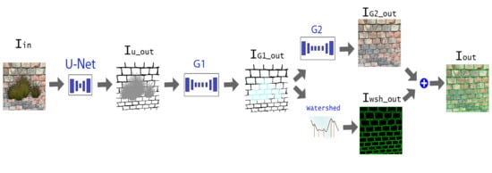
In this paper, we propose an end-to-end deep learning-based algorithm for masonry wall image analysis and virtual structure recovery. More specifically, given as input an image of a wall partially occluded by various irregular objects, our algorithm solves the following tasks in a fully automatic way (see also Figure 1):
- We detect the regions of the occluding objects, or other irregular wall components, such as holes, windows, damaged parts.
- We predict the brick-mortar pattern and the wall color texture in the hidden regions, based on the observable global wall texture.
- We extract the accurate brick contours both in the originally visible and in the artificially inpainted regions, leading to a strong structural representation of the wall.
First for the input wall images (Figure 1a) a U-Net [16] based algorithm is applied in a pre-processing step, whose output is a segmentation map with three classes, corresponding to brick, mortar, and irregular/occluded regions (see Figure 1b). This step is followed by an inpainting (completion) stage where two generative adversarial networks (GANs) are adopted consecutively. The first GAN completes the missing/broken mortar segments, yielding a fully connected mortar structure. Thereafter, the second GAN estimates the RGB color values of all pixels corresponding to the wall (Figure 1c). Finally, we segment the inpainted wall image using the watershed algorithm, yielding the accurate outlines of the individual brick instances (Figure 1d).
Due to the lack of existing masonry wall datasets usable for our purpose, we collected various images from modern and ancient walls and created our dataset in order to train the networks and validate our proposed approach.
Our motivation here is on one hand to develop a robust wall segmentation algorithm that can deal with different structural elements (stones, bricks ashlar, etc.), and accurately detect various kinds of possible occlusion or damage effects (cement plaster, biofilms [17]). The output of our segmentation step can support civil engineers and archaeologists while studying the condition and stability of the wall during maintenance, documentation or estimation of the necessary degree of protection. On the other hand, our proposed inpainting step can support the planning of the reconstruction or renovation work (both in virtual or real applications), by predicting and visualizing the possible wall segments in damaged or invisible regions.
In remote sensing images, the presence of clouds and their shadows can affect the quality of processing these images in several applications [18,19]. Hence, to make good use of such images, and as the background of the occluded parts follows the same pattern as the visible parts of the image, our algorithm can be trained in such cases to remove these parts and fill them with the expected elements (such as road network, vegetation and built-in structures).
We can summarize our contributions as follows:
- An end-to-end algorithm is proposed that encapsulates inpainting and a segmentation of masonry wall images, which may include occluded and/or damaged segments.
- We demonstrate the advantages of our approach in masonry wall segmentation and inpainting by detailed qualitative and quantitative evaluation.
- We introduce a new dataset for automatic masonry wall analysis.
The article is organized as follows: Section 2 summarizes previous works related to state-of-the-art wall image delineation and image inpainting algorithms; Section 3 shows the way we generate and augment our dataset; Section 4 introduces our proposed method in details; the training and implementation details are discussed in Section 5; Section 6 presents the experimental results; in Section 7 the results are discussed and further qualitative results are presented to support the validation of the approach; finally, Section 8 summarizes the conclusions of our research.
Preliminary stages of the proposed approach have been introduced in [20], which paper purely deals with brick segmentation, and in [21] where we constructed an initial inpainting model, which was validated mainly on artificial data samples. This article presents a more elaborated model, with a combination of multiple algorithmic components, which yield improved results and enable more extensive structural and visual analysis of masonry wall images. The present paper also provides extended quantitative and qualitative evaluation of the proposed approach regarding to occlusion detection, inpainting and brick segmentation, and we have compared it against several state-of-the-art algorithms on an expanded dataset, which includes several real-world samples. Moreover, as possible use-cases we also describe new application opportunities for archeologist in Section 7.
2. Background
Nowadays, there is an increasing need for efficient automated processing in cultural heritage applications, since manual documentation is time and resource consuming, and the accuracy is highly dependent on the experience of the experts. Developing an automatic method to analyze widely diverse masonry wall images is considered as a challenging task for various reasons [22]: issues should be addressed related to occlusions, lighting and shadows effects, we must expect a significant variety of possible shape, texture, and size parameters of the bricks and surrounding mortar regions, moreover, the texture can even vary within connected wall fragments, if it consists of multiple components built in different centuries from different materials.
Two critical issues in the above process are wall structure segmentation, and the prediction of the occluded/missing wall regions, which are jointly addressed in the paper. In this section, we give a brief overview about recent image segmentation algorithms used for masonry wall delineation. Thereafter, we discuss state-of-the-art of image inpainting techniques, focusing on their usability for the addressed wall image completing task.
2.1. Masonry Wall Delineation
The literature presents several wall image delineation algorithms, that achieved good results for specific wall types. Hemmleb et al. [23] proposed a mixture of object-oriented and pixel-based image processing technology for detecting and classifying the structural deficiencies, while Riveiro et al. [24] provided a color-based automated algorithm established on an improved marker-controlled watershed transform. However since the later algorithm concentrates on the structural analysis of quasi-periodic walls, it is limited to dealing with horizontal structures only; while most of the historical walls have various compositional modules. In the same vein, Noelia et al. [25] used an image-based delineation algorithm to classify masonry walls of ancient buildings, aiming to estimate the degree of required protection of these buildings as well. Enrique et al. [15] used 3D colored point clouds as input, then they generated a 2.5D map by projecting the data onto a vertical plane, and a Continuous Wavelet Transform (CWT) was applied on the depth map to obtain the outlines of the bricks. Bosche et al. [26] proposed a method that deals with 3D data points using local and global features to segment the walls into two sub-units representing the bricks and the joints. We have found that none of the mentioned approaches has been tested on much diverse wall image structures or textures. On the contrary, our primary aim in the presented research work was to deal with very different wall types and texture models at the same time with a high accuracy and precision. We have found that none of the mentioned approaches has been tested on much diverse wall image structures or textures. On the contrary, our primary aim in the presented research work was to deal with very different wall types and texture models at the same time with a high accuracy and precision.
2.2. Inpainting Algorithms
Image inpainting is a process where damaged, noisy, or missing parts of a picture are filled in to present a complete image. Existing image inpainting algorithms can be divided into blind or non-blind categories depending on whether the mask of the missing areas is automatically detected or manually given in advance to the algorithm. The state-of-the-art blind inpainting algorithms [27,28,29] only work under special circumstances: they focus for example on the removal of scratches or texts, and cannot deal with the cases with multiple occluding objects of complex shapes. Diffusion-based methods [30,31] and patch-based techniques [32,33,34] are traditional methods that use local image features or descriptors to inpaint the missing parts. However, such techniques lack the accuracy when the occluded parts are large, and they may produce miss-alignments for thin structures such as wall mortar (see Figure 2b–d, the results of a patch-based technique [34]).
Large datasets are needed to train the recently proposed deep learning models [35,36,37], which inpaint the images after training and learning a hidden feature representation. A generative multi-column convolutional neural network (GMCNN) model [38] was proposed with three sub-networks, namely the generator, the global and local discriminator, and a pre-trained VGG model [39]. This approach deals in parallel with global texture properties and local details by using a confidence driven reconstruction loss and diversified Markov random field regularization, respectively. A multi-output approach [40] is introduced to generate multiple image inpainting solutions with two GAN-based [41] parallel paths: the first path is reconstructive aiming at inpainting the image according to the Ground Truth map, while the other path is generative, which generates multiple solutions.
The EdgeConnect [42] approach uses a two-stage adversarial network that completes the missing regions according to an edge map generated in the first stage. Initial edge information should be provided to this algorithm which is based on either the Canny detector [43] or the Holistically-Nested Edge Detection algorithm (HED) [44]. However, if we apply this method for the masonry wall inpainting application, non of these two edges generators [43,44] can provide semantic structural information about the walls, since their performance is sensitive to the internal edges inside the brick or mortar regions, creating several false edges which are not related to the pattern of the wall structure. Moreover, the outputs of both edge generators [43,44] strongly depend on some threshold values, which should be adaptively adjusted over a wall image. To demonstrate these limitations, we show the outputs of the Canny edge detector (applied with two different threshold values), and the HED algorithm in Figure 3b–d for a selected masonry wall sample image. As explained later in details, one of the key components of our proposed method will be using an efficient, U-Net based delineation algorithm as a preprocessing step, whose output will approximate the manually segmented binary brick-mortar mask of the wall (see Figure 3e,f).
3. Dataset Generation
We have constructed a new dataset for training and evaluating the proposed algorithm, which contains images of facades and masonry walls, either from historical or contemporary buildings. As demonstrated in Figure 4, several different types of wall structures are included, for example three types of rubble masonry (Random, Square, Dry), and two types of ashlar (Fine, Rough). Even within a given class, the different samples may show highly variable characteristics, both regarding the parameters of the bricks (shape, size and color), and the mortar regions (thin, thick, or completely missing). In addition, the images are taken from different viewpoints in different lighting conditions, and contain shadow effects in some cases.
Using a large dataset plays an essential role to achieve efficient performance and generalization ability of deep learning methods. On the other hand, dataset generation is in our case particularly costly. First, for both training and quantitative evaluation of the brick-mortar segmentation step, we need to manually prepare a binary delineation mask (denoted henceforward by Iwall_ftr) for each wall image of the dataset, where as shown in the bottom row of Figure 4, background (black pixels) represents the regions of mortar, and foreground (white pixels) represents the bricks. In addition, for training and numerical quality investigation of the inpainting step, we also need to be aware of the accurate occlusion mask, and we have to know the original wall pattern, which could be observable without the occluding object. However, such sort of information is not available, when working with natural images with real occlusions or damaged wall parts, as shown in Figure 1.
For ensuring in parallel the efficiency and generality of the proposed approach, and the tractable cost of the training data generation process, we have used a combination of real and semi-synthetic images, and we took the advantages of various sorts of data augmentation techniques.
Our dataset is based on 532 different wall images of size , which are divided among the training set (310 images), and three test sets (222 images).
The training dataset is based on 310 occlusion-free wall images, where for each image we also prepared a manually segmented Iwall_ftr binary brick-mortar mask (see examples in Figure 4). For training, the occlusions are simulated using synthetic objects during data augmentation, so that the augmentation process consists of two phases:
- (i)
- Offline augmentation: 7 modified images are created for each base image using the following transformations: (a) horizontal flip, (b) vertical flip, (c) both vertical and horizontal flips, (d) adding Gaussian noise (e) randomly increasing the average brightness, (f) randomly decreasing the average brightness, and (g) adding random shadows.
- (ii)
- Online synthetic occlusion and data augmentation [45]: each image produced in the previous step is augmented online (during the training) by occluding the wall image Iwall with a random number (from 1 and 8) of objects (represented by Ioclud), chosen from a set of 2490 non_human samples of the Pascal VOC dataset [46]. With these parameter settings, we generated both moderately, and heavily occluded data samples. As demonstrated in Figure 5a,b, the result of this synthetic occlusion process is the Iin image, which is used as the input of the proposed approach. We also generate a target (Ground Truth) image for training and testing the image segmentation step, so that we combine the binary delineation map (Iwall_ftr) and the mask of the chosen occluding objects in a three-class image Iwall_ftr_oclud (see Figure 5b), which has the labels mortar (black), brick (white), and occlusion (gray). Afterward, we used the Imgaug library [47] to apply Gaussian noise, cropping/padding, perspective transformations, contrast changes, and affine transformations for each image.
Our test image collection is composed of three subsets:
- Test Set (1): We used 123 occlusion-free wall images and simulated occlusions by synthetic objects, as detailed later in Section 6. We only remark that here both the wall images and the synthetic objects were different from the ones used to augment the training samples. A few synthesized test examples are shown in the first rows of Figures 7 and 8.
- Test Set (2): We took 47 additional wall images with real occlusions and with available Ground Truth (GT) data in ancient sites of Budapest, Hungary. In these experiments, we mounted our camera to a fixed tripod, and captured image pairs of walls from the same positions with and without the presence of occluding objects (see the second rows in Figures 7 and 8).
- Test Set (3): For demonstrating the usability of the proposed techniques in real-life, we used 52 wall pictures:
- -
- 25 photos of various walls with real occlusions or damaged segments are downloaded from the web (see examples in Figure 1).
- -
- 27 masonry wall images from ancient archaeological sites in Syria are used to evaluate the inpainting and the segmentation steps of our proposed algorithm (see examples in Figure 12).
Note that since Test Set (1) and Test Set (2) contain both occluded and occlusion free images from the same site, they can be used in numerical evaluation of the proposed algorithm. On the other hand, Test Set (3) can be only used in qualitative surveys, however these images may demonstrate well the strength of the technique in real applications.
The wall images and the manually annotated masks used in the dataset are available at the website of the authors (http://mplab.sztaki.hu/geocomp/masonryWallAnalysis).
4. Proposed Approach
The main goals of the proposed method are (i) to automatically extract the individual brick instances of masonry wall images, (ii) to detect occluded or damaged wall segments, and (iii) to fill in the occluded/missing regions by a realistic prediction of the brick-mortar pattern.
The complete workflow is demonstrated in Figure 5. We assume that the input of the algorithm is a masonry wall image Iin which is partially occluded by one or several foreground objects. Our method provides multiple outputs: a color image of the reconstructed wall IG2_out, the binary brick-mortar delination map Iwsh_out of IG1_out, and the contours of the individual bricks. These outputs can be superimposed yielding a segmented color image Iout of Figure 5f.
The proposed approach is composed of three main stages as shown in Figure 5:
- Pre-processing stage (Figure 5b): taking an input image Iin two outputs are extracted: the delineation map of the observed visible bricks, and the mask of the occluding objects or damaged wall regions.
- Segmentation (Figure 5e): this stage aims to separate the mortar from the brick regions in the inpainted wall image, and extract the accurate brick contours.
Next we discuss the above three stages in details.
4.1. Pre-Processing Stage
The goal of this step is twofold: extracting the delineation structure by separation of the bricks from the mortar regions, and detecting the masks of possibly occluded wall parts which should be inpainted in the consecutive steps.
As shown in Figure 5b, the segmentation step is realized by a U-Net deep neural network [16], which consists of two main parts. The encoder part encodes the input image Iin into a compact feature representation, and the decoder part decodes these features into an image Iu_out that represents the predicted classes. In our implementation, a pre-trained Resnet50 [48] encoder is adopted in the encoder step, and a three-class image Iwall_ftr_oclud is used as the target of this network, whose labels represent brick (white), mortar (black) and occluded (gray) regions. From the Iu_out output, we derive two binary auxiliary images: Imask is the binary mask of the occluded pixels according to the prediction; and Iftr_mskd is a mask of the predicted bricks in the observed wall regions, where both the occluded and the brick pixels receive white labels, while the mortar pixels are black.
The network is trained using the Adam optimizer [49] over a joint loss that consists of a cross-entropy loss and a feature-matching loss term. The cross-entropy loss is applied to measure the difference between the probability distributions of the classes of the U-Net output Iu_out and the target Iwall_ftr_oclud, while the feature-matching loss contributes to the training of the Inpainting Stage as described in Section 4.2.1:
where and are regularization parameters which are modified during the training process. During the training phase, the value is calculated as the average of the -scores for the three classes, which is used as a confidence number for modifying the weights in the subsequent network component of the Inpainting Stage.
4.2. Inpainting Stage
This stage is composed of two main sub-steps. First, the Hidden Feature Generator completes the mortar pixels in the area covered by the white regions of the predicted Imask image, based on the mortar pattern observed in the Iftr_mskd mask. Second, the Image Completion step predicts the RGB color values of the pixels marked as occluded in the Imask image, depending on the color information of the Iwall_mskd image restricted to the non-occluded regions, and the structural wall features extracted from the IG1_out map within the occluded regions.
The inpainting stage is based on two different generative adversarial networks (GAN), where each one consists of generator/discriminator components. The generator architecture follows the model proposed by [50], which achieved impressive results in image-to-image translation [51] and in image inpainting [42]. The generator is comprised of encoders which down-sample the inputs twice, followed by residual blocks and decoders that upsample the results back to the original size. The discriminator architecture follows the PatchGAN [51], which determines whether overlapping image patches of size are real or not. In Figure 5, and represent the Generator and Discriminator of the Hidden Feature Generator stage, and and represent the Generator and Discriminator of the Image Completion stage.
4.2.1. Hidden Feature Generator
For creating the inputs of the first generator (), three images are used: the two output images of the pre-processing stage (Imask, Iftr_mskd), and Ig_in_mskd, which is the masked grayscale version of the input image. The output of , IG1_out represents the predicted wall structure, completing Iftr_mskd with brick outlines under the occlusion mask regions. The first discriminator predicts whether the predicted wall features are real or not, based on the inputs IG1_out and Iwall_ftr, both ones conditioned on the grayscale wall image Ig_wall.
The network is trained by the adversarial loss and the feature-matching loss, which are both weighted by the -score that reveals the accuracy of the pre-processing stage:
The adversarial loss is formulated as a two-player zero-sum game between the Generator network and the Discriminator network where the generator attempts to minimize the Equation (3), while the discriminator tries to maximize it:
The feature matching loss [42] is used to make the training process stable by forcing the generator to produce results with representations as close as possible to the real images. To increase the stability of the training stage, the Spectral Normalization (SN) [52] is applied for both the generator and the discriminator, scaling down the weight matrices by their respective largest singular values.
4.2.2. Image Completion
The input of the second generator, combines both the masked wall image (Iwall_mskd) and the output of the first generator (IG1_out). The aim of the generator is creating an output image IG2_out which is filled with predicted color information in the masked regions (see Figure 5d). The inputs of the discriminator are IG2_out and Iwall and its goal is to predict whether the color intensity is true or not. The network is trained over a joint loss that consists of loss, adversarial loss, perceptual loss, and style loss.
The adversarial loss has the same function as described in Section 4.2.1. The loss is applied to measure the distance between the algorithm output Iout and the target Iwall, which is applied in the non-masked area and in the masked area , respectively. While the perceptual loss [42,50] is applied to make the results perceptually more similar to the input images, the style loss [42,53] is used to transfer the input style onto the output. The TV loss is used to smooth the output in the border areas of the mask. Each loss is weighted by a regularization parameter as described by the following equation:
4.3. Segmentation Stage
The last stage of the proposed algorithm is responsible for extracting the accurate outlines of the brick instances, relying on the previously obtained Hidden Feature Generator delineation map IG1_out. Although the delineation maps are quite reliable, they might be noisy near to the brick boundaries, and we can observe that some bricks are contacting, making simple connected component analysis (CCA) based separation prone to errors. To overcome these problems, we apply a marker based watershed [54] segmentation for robust brick separation.
The dataflow of the segmentation stage is described at Figure 6, which follows the post-processing step in [20], where first, we calculate the inverse distance transform (IDT) map of the obtained delineation map (IG1_out). Our aim is to extract a single compact seed region within each brick instance, which can be used as internal marker for the watershed algorithm. Since the IDT map may have several false local minima, we apply the H–minima transform [55], which suppresses all minima under a given H-value. Then, we apply flooding from the obtained H–minima regions, so that we consider the inverse of IG1_out (i.e., all mortar or non-wall pixels) as an external marker map, whose pixels cannot be assigned to any bricks. Finally the obtained brick contours can be displayed over the Image Completion output (see Iout).
5. Training and Implementation Details
We implemented the proposed method using Python and PyTorch. An NVIDIA GTX1080Ti GPU with 11 GB RAM was used to speed up the calculations. All networks in the Pre-Processing and Inpainting stages are trained using images with a batch size of four. For the training phase, the three sub-networks can interact through shared dependencies in their loss functions. However, this model leads to a highly complex optimization problem, with large computational and memory requirements. Particularly, we had to manage to fit into the GPU memory during the training process. For these reasons, in the initial training phase, the three networks were separately trained, providing an efficient initial weight-set for the upcoming joint optimization steps. Thereafter the first two networks were trained together, so that the the -score of the U-Net output was used as a confidence value to weight the loss function of (see Equation (2) in Section 4.2.1), and the feature matching loss of was used to update the U-Net weights (see Equation (1) in Section 4.1). For all stages in the network the Adam optimizer parameters were set as and . The hyperparameters of regularization were set based on experiments, and we used the following settings:
- (1)
- Pre-Processing Stage: we choose for the first epochs , , and for the last epochs , .
- (2)
- Inpainting Stage:
- (i)
- Hidden Feature Generator network: , .
- (ii)
- Image Completion network: , , , , , .
- (3)
- Segmentation Stage: H-value pixels.
6. Results
We evaluated the proposed algorithm step by step, both via quantitative tests and an extensive qualitative survey, using the test data collection introduced in Section 3. Our test data collection consists of three test sets, where the first two sets can be used in quantitative evaluation.
Test Set (1) is constructed by simulating occlusions on 123 different (occlusion-free) wall images, so that neither the wall images nor the occluding objects have been used during the training stage. More specifically, as occluding objects, we used a set of 545 different person images from the Pascal VOC dataset [46], and by random scaling we ensured that each one of the generated synthetic objects covers from to of the area of the wall image (see examples in the first rows of Figure 7 and Figure 8). For each base wall image of this test subset, we generated five test images (Iin), so that the number of the occluding objects varies from 1 to 5 in a given test image. As a result, the augmented image set of Test Set (1) was divided into five groups depending on the number of the occluding objects.
Test Set (2) contains image pairs of walls taken from the same camera position, where the first image contains real occluding objects, while the second image shows only the pure wall without these objects (see the second rows in Figure 7 and Figure 8). In this way the second image can be considered as a Ground Truth for the inpainting technique. We recall here that the process for capturing these images was discussed in Section 3.
In the following sections, we present evaluation results for each stage of the algorithm.
6.1. Occlusion Detection in the Pre-Processing Stage
The pre-processing stage classifies the pixels of the input image into three classes: brick, mortar, and regions of occluding object. Since brick-mortar separation is also part of the final segmentation stage, we will detail that issue later during the discussion of Section 6.3, and here we only focus on the accuracy of occlusion mask extraction.
Both for Test Set (1) and Test Set (2), we compare the occlusion mask estimation provided by the U-Net (i.e., gray pixels in Iu_out) to the corresponding Ground Truth (GT) mask derived from the reference map Iwall_ftr_oclud, as demonstrated in Figure 5b. Note that for images from Test Set (1), this mask is automatically derived during synthetic data augmentation in the same manner as described for training data generation in Section 3 (ii). On the other hand, for Test Set (2) the GT masks of the occluding (real) objects are manually segmented.
Taking the GT masks as reference, we calculate the pixel-level Precision (Pr) and Recall (Rc) values for the detected occlusion masks, and derive the -score as the harmonic mean of Pr and Rc.
The results are reported in Table 1, where for Test Set (1) (Synthetic) we also present separately the results within the five sub-groups depending on the number of occluding objects. The last row (Real) corresponds to the results in Test Set (2). For qualitative demonstration of this experiment, in Figure 7 we can compare the silhouette masks of the occluding objects extracted from the U-Net network output, and the Ground Truth occlusion mask (see a sample image from the Synthetic Test Set (1) in the first row, and one from the Real Test Set (2) in the second row).
The numerical results in Table 1 confirm the efficiency of our algorithm in detecting the occluded regions of the images. For all considered configurations, the recall rates of the occluded areas surpass 83%, ensuring that the real outlier regions (which should be inpainted) are found with a high confidence rate. Since the network also extracts some false occlusions, the measured -scores are between 58% and 85%. However, the observed relatively lower precision does not cause critical problems in our application, since false positives only implicate some unnecessarily inpainted image regions, but during the qualitative tests of the upcoming inpainting step, we usually did not notice visual errors in these regions (see the first
column in Figure 15, and its discussion in Section 7).
We can also notice from Table 1, that by increasing the number of occluding objects, the precision (thus also the -score) increases due to less false alarms. Based on further qualitative analysis (see also Figure 15) we can confirm, that the U-Net network can detect the occluding objects with high accuracy as nearly all of the virtually added irregular objects or the real occluding objects have been correctly detected.
6.2. Quantitative Evaluation of the Inpainting Stage
In this stage, two output maps are extracted sequentially. The first one is the output which is a binary classification mask showing the prediction of the mortar and the brick regions in the occluded areas. Figure 8c shows the output of where the blue pixels indicate the predicted mortar pixels in the masked region, while the Ground Truth mortar regions are provided as a reference in Figure 8d. Since the result of this step is a structure delineation mask, which directly affects the brick segmentation stage, corresponding numerical results will be presented in Section 6.3.
The second result of this stage is the output, which is an inpainted color image IG2_out that should be compared to the original occlusion-free wall image Iwall. For evaluating this step, we compared our method to state-of-the-art inpainting algorithms. Since (as mentioned in Section 2.2) existing blind image inpainting algorithms have significantly different purposes from our approach (such as text or scratch removal), we found a direct comparison with them less relevant. Therefore, in this specific comparative experiment, we used our approach in a non-blind manner and compared it to three non-blind algorithms: the Generative Multi-column Convolutional Neural Network (GMCNN) [38], the Pluralistic Image Completion [40], and the Canny based EdgeConnect [42].
In the training stage, for a fair comparison, an offline augmentation step was used in order to train all algorithms on the same dataset. We used the Augmentor library [56] for randomly rotating the images up to , and randomly applying horizontal and vertical flipping transforms, zooming up to of the image size, and changing the contrast of the images, yielding altogether 10,000 augmented images. Moreover, during the training phase, for simulating the missing pixels (i.e., holes or occluded regions that should be inpainted in the images), we used the same masks for all inpainting algorithms. These masks are derived from two different sources: (i) Irregular external masks from a publicly available inpainting mask set [35] which contains masks with and without holes close to the image borders, with a varying hole-to-image area ratios from 0% to . (ii) Regular square shaped masks of fixed sizes ( of total image pixels) centered at a random location within the image.
In the evaluation stage, randomly chosen external masks were adopted from the mask set proposed by [35]. More specifically, we chose 5 subsets of masks according to their hole-to-image area ratios: ((0%, ], (10%, ], (20%, ], (30%, ], (40%, ]). Thereafter, we overlaid occlusion-free wall images from the Test Set (1) with the selected/generated masks, to obtain the input images of all inpainting algorithms during this comparison (see also Figure 9, first row).
As mentioned in [35], there is no straightforward numerical metric to evaluate the image inpainting results due to the existence of many possible solutions. Nevertheless, we calculated the same evaluation metrics as usually applied in the literature [35,42]:
Table 2 shows the numerical results of the inpainting algorithms for each mask subset, and in Figure 9 we can visually compare the results of the considered GMCNN, Pluralistic and EdgeConnect methods to the proposed approach and to the Ground Truth.
Both the qualitative and quantitative results demonstrate that our approach outperforms the GMCNN and Pluralistic techniques, while the numerical evaluation rates of the proposed approach are very similar to EdgeConnect. While our FID-Scores (which is considered as the most important parameter) are slightly better, yet we found that these results do not provide a reliable basis for comparison.
For this reason, we have also performed a qualitative comparative survey between EdgeConnect and the proposed method so that for 25 different input images we showed the output pairs in a random order to 93 independent observes and asked them to choose the better ones without receiving any information about the generating method, and without using any time limitation. The participants of the survey were selected having different job backgrounds, but most of them were working in the fields of architecture or archaeology (Figure 10a displays the distribution of the different fields of expertize among the participants). Figure 10b shows for each test image the percentage of the answers, which marked our proposed algorithm’s output better than EdgeConnect’s result. This survey proved the clear superiority of our proposed method, since in 18 images out of 25 our approach received more votes than the reference method, and even in cases when our technique lost, the margin was quite small, which means that both approaches were judged as almost equally good. By summarizing all votes on all images, our method outperformed the Canny-based EdgeConnect with a significant margin: 58.59% vs. 41.41%.
The above tendencies are also demonstrated in Figure 11 for two selected images. On one hand, the numerical results of EdgeConnect are very close to our figures (EdgeCon/Ours PSNR: 27.02/25.95, SSIM: 86.67/85.16, L1: 1.46/1.67). On the other hand, we can visually notice that our algorithm reconstructs a significantly better mortar network, which is a key advantage for archaeologist aiming to understand how the wall was built. The superiority of our algorithm over the Canny-based EdgeConnect approach may be largely originated from the fact, that our method is trained to make a clear separation between the mortar and the bricks in the pre-processing stage, even in difficult situations such as densely textured wall images or walls with shadows effects. In such cases the Canny detector provides notably noisy and incomplete edge maps which fools the consecutive inpainting step.
6.3. Quantitative Evaluation of the Segmentation Stage
We evaluated the results of the brick segmentation step for the images of Test Set (1) (synthetic—123 images), and Test Set (2) (real—47 images). First, since in these test sets, the background wall images are also available, we measure the segmentation accuracy for the occlusion-free wall images. Thereafter, for the synthetic test set, we investigate the performance as a function of the number of occluding objects, while we also test the algorithm for the images with real occlusions (Test Set (2)). Note that in this case, apart from investigating the accuracy of the segmentation module, we also evaluate indirectly the accuracy of brick segment prediction in the occluded regions.
In this evaluation step, we measure the algorithm’s performance in two different ways: we investigate how many bricks have been correctly (or erroneously) detected, and also assess the accuracy of the extracted brick outlines. For this reason, we calculate both (i) object level and (ii) pixel level metrics. First of all, an unambiguous assignment is taken between the detected bricks (DB) and the Ground Truth (GT) bricks (i.e., every GT object is matched to at most one DB candidate). To find the optimal assignment we use the Hungarian algorithm [59], where for a given DB and GT object pair the quality of matching is proportional to the intersection of union (IOU) between them, and we only take into account the pairs that have IOU higher than a pre-defined threshold 0.5. Thereafter, object and pixel level matching rates are calculated as follows:
- (i)
- At object (brick) level, we count the number of True Positive (TP), False Positive (FP) and False Negative (FN) hits, and compute the object level precision, recall and F1-score values. Here TP corresponds to the number detected bricks (DBs) which are correctly matched to the corresponding GT objects, FP refers to DBs which do not have GT pair, while FN includes GT objects without any matches among the DBs.
- (ii)
- At pixel level, for each correctly matched DB-GT object pair, we consider the pixels of their intersection as True Positive (TP) hits, the pixels that are in the predicted brick but not in the GT as False Positive (FP), and pixels of the GT object missing from the DB as False Negative (FN). Thereafter we compute the pixel level evaluation metrics precision, recall and F1-score and the intersection of unions (IOU). Finally the evaluation metric values for the individual objects are averaged over all bricks, by weighting each brick with its total area.
Table 3 shows the quantitative object and pixel level results of the segmentation stage. The results confirm the efficiency of our algorithm for brick prediction in the occluded regions, as the F1-scores at both brick and pixel levels are in each case above 67%. Note that the observed results are slightly weaker for the images with real occlusions (Test Set (2)), which is caused by two factors. First, in these images the area of the occluding objects is relatively large (more than 30%). Second, the occluding objects form large connected regions, which yields a more challenging scenario than adding 5 smaller synthetic objects to different parts of the wall image, as we did in the experiment with artificial occlusions.
It is important to notice that the Ground Truth is not the only reference that our result could be compared to, as there might be many valid realistic solutions. However, both the quantitative results and the qualitative examples show that the proposed method can generally handle very different masonry types with high efficiency.
The prediction results show graceful degradation in cases of more challenging samples, such as random masonry, as the wall could take any pattern and all the predicting patterns in the occluding regions can be considered as a real pattern (see Figure 8). Expected outputs are more definite when we are dealing with square rubble masonry or ashlar masonry categories where the pattern is specific and well predictable (see the first and third rows in Figure 12).
7. Discussion
In this section, we discuss further qualitative results demonstrating the usability of the proposed approach in various real application environments.
Figure 12 shows the results of occlusion detection, brick-mortar structure segmentation and prediction, and inpainting for real images from Test Set (3). The first image displays a wall from Budapest, where a street plate occludes a few bricks. Here exploiting the quite regular wall texture and the high image contrast, all the three demonstrated steps proved to be notably efficient. The second and third images contain ancient masonry walls from Syria occluded by some vegetation. We can observe that several plants were detected as occluded regions and appropriately inpainted, while the wall’s structure has also been correctly delineated and reconstructed. Note that such delineation results (i.e., outputs of the G1 component) can be directly used in many engineering and archeology applications, such as analysis of excavation sites or maintenance of buildings. On the other hand, we can also notice a number of further issues in these images, which are worth for attention. First, due to the low contrast of the second image (middle row), not all mortar regions could have been extracted, but this fact does not cause significant degradation in the inpainting results. Second, some vegetation regions are left unchanged, which artifact can only be eliminated with involving further features during the training. Third, in the last row, the algorithm also filled in a door, which was identified as an occluded or damaged wall region. To avoid such phenomena, special elements, such as doors, windows or ledges could be recognized by other external object recognizer modules [60], and masked during the inpainting process.
Figure 13 shows further brick segmentation results for some occlusion-free archeological wall images (also from Test Set (3)), which have challenging structures with diverse brick shapes and special layouts. Moreover the first and second images also have some low contrasted regions which makes brick separation notably difficult. First we can observe that the delineation step (second column) is highly successful even under these challenging circumstances. Moreover, even in cases where touching bricks were merged into a single connected blob in the delineation map, the watershed based segmentation step managed to separate them as shown in the final output (third column), which is notably close to the manually marked Ground Truth (fourth column).
Next we introduce a possible extension of our algorithm which offers an additional feature, making our approach unique among the existing inpainting techniques. We give the users the flexibility to draw and design their own perspective of the mortar-brick pattern in the hidden (occluded) areas via simple sketch drawings. Then the inpainting stage uses this manually completed delineation map as input to produce the colored version of the reconstructed wall image, whose texture style follows the style of the unoccluded wall segments, meantime the pattern defined by the sketch drawing also appears in the inpainted region. This feature allows the archaeologists to easily imagine the wall structure of the hidden parts which might also help in reassembling the wall elements through a better visualization. Figure 14 demonstrates the above described process. First, we assume that some regions of the wall are hidden (see white pixels in Figure 14a). Thereafter, we allow the user to modify the delineation map by hand, adding new mortar regions which are shown in red in Figure 14b. Finally the algorithm completes the wall elements with realistic results (Figure 14c), which works even if the user draws unexpected or non-realistic wall structures as shown in the second and third rows of the figure.
For a brief summary, Figure 15 demonstrates the results of our proposed algorithm step by step. The first row shows selected input wall images which contain various occluding objects (synthetic occluding objects in the first two columns, and real ones in the last two columns). The second row displays the output of the pre-processing stage where occluding objects are shown in gray, and bricks in white. The third row is the output where the predicted mortar pixels under the occluded regions are shown with blue color, and the forth row displays the output of the inpainting stage which is an inpainted color image. The fifth row shows the output of the brick segmentation stage, which is followed by the Ground Truth, i.e., the original wall image without any occluding objects.
In the first example (see the first column), the pre-processing step predicts some segments of the yellow line as occluding objects, due to their outlier color values compared to other segments of the wall. The false positive occlusion predictions naturally affect the final results, however, as shown by this example, the inpainting result is yet realistic, and the brick segmentation output is almost perfect here. In the second and third columns, the bricks of the walls follow less regular patterns, but even in these complex cases, the proposed algorithm predicts efficient mortar-bricks maps and realistic inpainted color images of the walls. Moreover, the brick segmentation results are of high quality in the non-occluded regions, despite the high variety in the shapes of the brick components. The wall in the fourth (last) column follows a periodic and highly contrasted pattern, thus the pre-processing stage is able to separate the mortar, brick and occlusion regions very efficiently. Some minor mistakes appear only in the bottom-right corner, where the color of the occluding person’s lower leg is quite similar the one of the frequent brick colors in the image.
Based on the above discussed qualitative and quantitative results, we can conclude that our algorithm provides high quality inpainting and segmentation outputs for different wall patterns and structures, in cases of various possible occluding objects.
8. Conclusions
This paper introduced a new end-to-end wall image segmentation and inpainting method. Our algorithm detects the occluded or damaged wall parts based on a single image, and inpaints the missing segment with the expected wall elements. In addition, the method also provides an instance level brick segmentation output for the inpainted wall image. Our method consists of three stages. The first, pre-processing stage adopts a U-Net based module, which separates the brick, mortar and occluded regions of the input image. This preliminary segmentation serves as input of the inpainting stage, which consists of two GAN based networks: the first one is responsible for wall structure compilation; while the second one for the color image generation task. The last stage uses the watershed algorithm which fulfills accurate brick segmentation for the complete wall. We have shown by various quantitative and qualitative experiments that for the selected problem the proposed approach significantly surpasses the state-of-the-art general inpainting algorithms, moreover, the segmentation process is highly general and largely robust against various artifacts appearing in real-life applications. As future work, we are planning the extend the image database, and test various network architectures backbones, loss functions and training strategies which can lead to even improved results.
Author Contributions
All authors contributed to the conceptualization, methodology, and writing—editing the paper. Further specific contributions: software, Y.I.; data acquisition, Y.I.; validation and comparative state-of-the-art analysis, Y.I.; writing—original draft preparation, Y.I.; writing—review and editing, C.B.; supervision and funding acquisition C.B., B.N. All authors have read and agreed to the published version of the manuscript.
Funding
This work was supported by the Artificial Intelligence National Laboratory (MILAB); by the National Research, Development and Innovation Fund, under grants K-120233 and 2018-2.1.3-EUREKA-2018-00032; by the European Union and the Hungarian Government from the project ‘Thematic Fundamental Research Collaborations Grounding Innovation in Informatics and Infocommunications’ under grant number EFOP-3.6.2-16-2017-00013 (B.N.), and from the project ‘Intensification of the activities of HU-MATHS-IN—Hungarian Service Network of Mathematics for Industry and Innovation’ under grant number EFOP-3.6.2-16-2017-00015 (C.B.); by the ÚNKP-20-4 New National Excellence Program of the Ministry of Human Capacities (B.N.); by the National Excellence Program under Grant 2018-1.2.1-NKP-00008, and by the Michelberger Master Award of the Hungarian Academy of Engineering (C.B.).
Acknowledgments
The authors thank Gábor Bertók from the Archaeological GIS Laboratory of the Péter Pázmany Catholic University, Hungary, for contributing to our dataset acquisition process via provision of the Syrian images, and for his kind remarks and advices regarding the main directions of the research work.
Conflicts of Interest
The authors declare no conflict of interest. The funders had no role in the design of the study; in the collection, analyses, or interpretation of data; in the writing of the manuscript, or in the decision to publish the results.
Abbreviations
The following abbreviations are used in this manuscript:
| CH | Cultural Heritage |
| DCH | Digital Cultural Heritage |
| DL | Deep Learning |
| ML | Machine Learning |
| GAN | Generative Adversarial Networks |
| HED | Holistically-Nested Edge Detection |
| IDT | inverse distance transform |
| GT | Ground Turth |
| Pr | Precision |
| Rc | Recall |
| TP | True Positive |
| FP | False Positive |
| FN | False Negative |
| IOU | intersection of union |
| PSNR | Peak Signal-to-Noise Ratio |
| SSIM | Structural Similarity Index |
| FID | Fréchet Inception Distance |
References
- Pierdicca, R.; Paolanti, M.; Matrone, F.; Martini, M.; Morbidoni, C.; Malinverni, E.S.; Frontoni, E.; Lingua, A.M. Point Cloud Semantic Segmentation Using a Deep Learning Framework for Cultural Heritage. Remote Sens. 2020, 12, 1005. [Google Scholar] [CrossRef] [Green Version]
- Gallwey, J.; Eyre, M.; Tonkins, M.; Coggan, J. Bringing Lunar LiDAR Back Down to Earth: Mapping Our Industrial Heritage through Deep Transfer Learning. Remote Sens. 2019, 11, 1994. [Google Scholar] [CrossRef] [Green Version]
- de Lima-Hernandez, R.; Vergauwen, M. A Hybrid Approach to Reassemble Ancient Decorated Block Fragments through a 3D Puzzling Engine. Remote Sens. 2020, 12, 2526. [Google Scholar] [CrossRef]
- Teruggi, S.; Grilli, E.; Russo, M.; Fassi, F.; Remondino, F. A Hierarchical Machine Learning Approach for Multi-Level and Multi-Resolution 3D Point Cloud Classification. Remote Sens. 2020, 12, 2598. [Google Scholar] [CrossRef]
- Eramian, M.G.; Walia, E.; Power, C.; Cairns, P.A.; Lewis, A.P. Image-based search and retrieval for biface artefacts using features capturing archaeologically significant characteristics. Mach. Vis. Appl. 2016, 28, 201–218. [Google Scholar] [CrossRef] [PubMed] [Green Version]
- Prasomphan, S.; Jung, J.E. Mobile Application for Archaeological Site Image Content Retrieval and Automated Generating Image Descriptions with Neural Network. Mob. Netw. Appl. 2017, 22, 642–649. [Google Scholar] [CrossRef]
- van der Maaten, L.; Boon, P.; Lange, G.; Paijmans, J.; Postma, E. Computer Vision and Machine Learning for Archaeology. 2006. Available online: https://publikationen.uni-tuebingen.de/xmlui/bitstream/handle/10900/61550/CD49_Maaten_et_al_CAA2006.pdf (accessed on 27 November 2020).
- Rasheed, N.A.; Nordin, M.J. Classification and reconstruction algorithms for the archaeological fragments. J. King Saud Univ.-Comput. Inf. Sci. 2018, 32, 883–894. [Google Scholar] [CrossRef]
- Hadjiprocopis, A.; Ioannides, M.; Wenzel, K.; Rothermel, M.; Johnsons, P.S.; Fritsch, D.; Doulamis, A.; Protopapadakis, E.; Kyriakaki, G.; Makantasis, K.; et al. 4D reconstruction of the past: The image retrieval and 3D model construction pipeline. In Proceedings of the Second International Conference on Remote Sensing and Geoinformation of the Environment (RSCy2014), Paphos, Cyprus, 7–10 April 2014; Hadjimitsis, D.G., Themistocleous, K., Michaelides, S., Papadavid, G., Eds.; International Society for Optics and Photonics, SPIE: Bellingham, WA, USA, 2014; Volume 9229, pp. 331–340. [Google Scholar] [CrossRef]
- Hashimoto, R.; Koyama, T.; Kikumoto, M.; Saito, T.; Mimura, M. Stability Analysis of Masonry Structure in Angkor Ruin Considering the Construction Quality of the Foundation. J. Civ. Eng. Res. 2014, 4, 78–82. [Google Scholar]
- Kılıç Demircan, R.; Ünay, A.İ. Structural Stability Analysis of Large-Scale Masonry Historic City Walls. In Proceedings of the 3rd International Sustainable Buildings Symposium (ISBS 2017), Dubai, UAE, 15–17 March 2017; Fırat, S., Kinuthia, J., Abu-Tair, A., Eds.; Springer: Cham, Switzerland, 2018; pp. 384–395. [Google Scholar]
- Shen, Y.; Lindenbergh, R.; Wang, J.; Ferreira, V.G. Extracting Individual Bricks from a Laser Scan Point Cloud of an Unorganized Pile of Bricks. Remote Sens. 2018, 10, 1708. [Google Scholar] [CrossRef] [Green Version]
- Bolhassani, M.; Rajaram, S.; Hamid, A.A.; Kontsos, A.; Bartoli, I. Damage detection of concrete masonry structures by enhancing deformation measurement using DIC. In Nondestructive Characterization and Monitoring of Advanced Materials, Aerospace, and Civil Infrastructure 2016; Yu, T., Gyekenyesi, A.L., Shull, P.J., Wu, H.F., Eds.; International Society for Optics and Photonics, SPIE: San Diego, CA, USA, 2016; Volume 9804, pp. 227–240. [Google Scholar] [CrossRef]
- Ali, L.; Khan, W.; Chaiyasarn, K. Damage Detection and Localization in Masonry Structure Using Faster Region Convolutional Networks. Int. J. GEOMATE 2019, 17, 98–105. [Google Scholar] [CrossRef]
- Valero, E.; Bosché, F.; Forster, A.; Hyslop, E. Historic Digital Survey: Reality Capture and Automatic Data Processing for the Interpretation and Analysis of Historic Architectural Rubble Masonry. In Structural Analysis of Historical Constructions; Aguilar, R., Torrealva, D., Moreira, S., Pando, M.A., Ramos, L.F., Eds.; Springer: Cham, Switzerland, 2019; pp. 388–396. [Google Scholar]
- Ronneberger, O.; Fischer, P.; Brox, T. U-Net: Convolutional Networks for Biomedical Image Segmentation. In Medical Image Computing and Computer-Assisted Intervention; Springer: Cham, Switzerland, 2015; Volume 9351, pp. 234–241. [Google Scholar]
- Suchocki, C.; Damięcka-Suchocka, M.; Katzer, J.; Janicka, J.; Rapiński, J.; Stałowska, P. Remote Detection of Moisture and Bio-Deterioration of Building Walls by Time-Of-Flight and Phase-Shift Terrestrial Laser Scanners. Remote Sens. 2020, 12, 1708. [Google Scholar] [CrossRef]
- Duan, C.; Pan, J.; Li, R. Thick Cloud Removal of Remote Sensing Images Using Temporal Smoothness and Sparsity Regularized Tensor Optimization. Remote Sens. 2020, 12, 3446. [Google Scholar] [CrossRef]
- Dai, P.; Ji, S.; Zhang, Y. Gated Convolutional Networks for Cloud Removal From Bi-Temporal Remote Sensing Images. Remote Sens. 2020, 12, 3427. [Google Scholar] [CrossRef]
- Ibrahim, Y.; Nagy, B.; Benedek, C. CNN-Based watershed Marker Extraction for Brick Segmentation in Masonry Walls. In Proceedings of the International Conference Image Analysis and Recognition, Waterloo, ON, Canada, 27–29 August 2019; pp. 332–344. [Google Scholar]
- Ibrahim, Y.; Nagy, B.; Benedek, C. A GAN-based Blind Inpainting Method for Masonry Wall Images. In Proceedings of the International Conference on Pattern Recognition, Milan, Italy, 10–15 January 2021. [Google Scholar]
- Sithole, G. Detection of bricks in a masonry wall. Int. Arch. Photogramm. Remote Sens. Spat. Inf. Sci. 2008, XXXVII, 567–572. [Google Scholar]
- Hemmleb, M.; Weritz A, F.; Schiemenz B, A.; Grote C, A.; Maierhofer, C. Multi-spectral data acquisition and processing techniques for damage detection on building surfaces. In Proceedings of the ISPRS Commission V Symposium, Dresden, Germany, 25–27 September 2006; pp. 1–6. [Google Scholar]
- Riveiro, B.; Conde, B.; Gonzalez, H.; Arias, P.; Caamaño, J. Automatic creation of structural models from point cloud data: The case of masonry structures. ISPRS Ann. Photogramm. Remote Sens. Spat. Inf. Sci. 2015, II-3/W5, 3–9. [Google Scholar] [CrossRef] [Green Version]
- Oses, N.; Dornaika, F.; Moujahid, A. Image-Based Delineation and Classification of Built Heritage Masonry. Remote Sens. 2014, 6, 1863–1889. [Google Scholar] [CrossRef] [Green Version]
- Bosché, F.; Valero, E.; Forster, A.; Wilson, L.; Leslie, A. Evaluation of historic masonry substrates: Towards greater objectivity and efficiency. Constr. Build. Mater. 2016, 102, 592–600. [Google Scholar] [CrossRef]
- Xie, J.; Xu, L.; Chen, E. Image Denoising and Inpainting with Deep Neural Networks. In Advances in Neural Information Processing Systems 25 (NIPS); MIT Press: Cambridge, MA, USA, 2012; pp. 341–349. [Google Scholar]
- Liu, Y.; Pan, J.; Su, Z. Deep Blind Image Inpainting. In Proceedings of the Intelligence Science and Big Data Engineering, Visual Data Engineering, Nanjing, China, 17–20 October 2019; pp. 128–141. [Google Scholar]
- Köhler, R.; Schuler, C.; Schölkopf, B.; Harmeling, S. Mask-Specific Inpainting with Deep Neural Networks. In Proceedings of the German Conference on Pattern Recognition, LNCS, Munster, Germany, 2–5 September 2014; pp. 523–534. [Google Scholar]
- Esedoglu, S.; Shen, J. Digital inpainting based on the Mumford-Shah-Euler image model. Eur. J. Appl. Math. 2002, 13, 353–370. [Google Scholar] [CrossRef] [Green Version]
- Liu, D.; Sun, X.; Wu, F.; Li, S.; Zhang, Y. Image Compression with Edge-Based Inpainting. IEEE Trans. Circuits Syst. Video Technol. 2007, 17, 1273–1287. [Google Scholar] [CrossRef]
- Barnes, C.; Shechtman, E.; Finkelstein, A.; Goldman, D.B. PatchMatch: A Randomized Correspondence Algorithm for Structural Image Editing. ACM Trans. Graph. 2009, 28, 24. [Google Scholar] [CrossRef]
- Darabi, S.; Shechtman, E.; Barnes, C.; Goldman, D.B.; Sen, P. Image Melding: Combining Inconsistent Images using Patch-based Synthesis. ACM Trans. Graph. 2012, 31, 82:1–82:10. [Google Scholar] [CrossRef]
- Martin, D.; Fowlkes, C.; Tal, D.; Malik, J. A Database of Human Segmented Natural Images and its Application to Evaluating Segmentation Algorithms and Measuring Ecological Statistics. In Proceedings of the 8th International Conference Computer Vision, Vancouver, BC, Canada, 7–14 July 2001; Volume 2, pp. 416–423. [Google Scholar]
- Liu, G.; Reda, F.A.; Shih, K.J.; Wang, T.C.; Tao, A.; Catanzaro, B. Image Inpainting for Irregular Holes Using Partial Convolutions. In Proceedings of the European Conference on Computer Vision (ECCV), Munich, Germany, 8–14 September 2018. [Google Scholar]
- Yu, J.; Lin, Z.; Yang, J.; Shen, X.; Lu, X.; Huang, T. Free-Form Image Inpainting With Gated Convolution. In Proceedings of the International Conference on Computer Vision (ICCV), Seoul, Korea, 27 October–2 November 2019; pp. 4470–4479. [Google Scholar]
- Pathak, D.; Krähenbühl, P.; Donahue, J.; Darrell, T.; Efros, A.A. Context Encoders: Feature Learning by Inpainting. In Proceedings of the IEEE Conference on Computer Vision and Pattern Recognition (CVPR), Las Vegas, NV, USA, 27–30 June 2016; pp. 2536–2544. [Google Scholar]
- Wang, Y.; Tao, X.; Qi, X.; Shen, X.; Jia, J. Image Inpainting via Generative Multi-column Convolutional Neural Networks. arXiv 2018, arXiv:1810.08771. [Google Scholar]
- Simonyan, K.; Zisserman, A. Very Deep Convolutional Networks for Large-Scale Image Recognition. arXiv 2014, arXiv:1409.1556. [Google Scholar]
- Zheng, C.; Cham, T.; Cai, J. Pluralistic Image Completion. In Proceedings of the IEEE Conference on Computer Vision and Pattern Recognition (CVPR), Long Beach, CA, USA, 16–20 June 2019; pp. 1438–1447. [Google Scholar]
- Goodfellow, I.; Pouget-Abadie, J.; Mirza, M.; Xu, B.; Warde-Farley, D.; Ozair, S.; Courville, A.; Bengio, Y. Generative Adversarial Nets. In Advances in Neural Information Processing Systems; MIT Press: Cambridge, MA, USA, 2014; Volume 27, pp. 2672–2680. [Google Scholar]
- Nazeri, K.; Ng, E.; Joseph, T.; Qureshi, F.; Ebrahimi, M. EdgeConnect: Generative Image Inpainting with Adversarial Edge Learning. In Proceedings of the International Conference on Computer Vision Workshop (ICCVW), Seoul, Korea, 27–28 October 2019; pp. 3265–3274. [Google Scholar]
- Canny, J. A computational approach to edge-detection. IEEE Trans. Pattern Anal. Mach. Intell. 1986, 8, 679–698. [Google Scholar] [CrossRef] [PubMed]
- Xie, S.; Tu, Z. Holistically-Nested Edge Detection. In Proceedings of the IEEE International Conference on Computer Vision (ICCV), Santiago, Chile, 7–13 December 2015; pp. 1395–1403. [Google Scholar]
- Sárándi, I.; Linder, T.; Arras, K.O.; Leibe, B. How Robust is 3D Human Pose Estimation to Occlusion? In Proceedings of the IEEE/RSJ International Conference Intelligent Robots and Systems Workshop (IROSWS), Madrid, Spain, 1–5 October 2018. [Google Scholar]
- Everingham, M.; Van Gool, L.; Williams, C.K.I.; Winn, J.; Zisserman, A. The PASCAL Visual Object Classes Challenge 2012 (VOC2012) Results. Available online: http://host.robots.ox.ac.uk/pascal/VOC/voc2012/ (accessed on 27 November 2020).
- Jung, A.B.; Wada, K.; Crall, J.; Tanaka, S.; Graving, J.; Reinders, C.; Yadav, S.; Banerjee, J.; Vecsei, G.; Kraft, A.; et al. Imgaug. 2020. Available online: https://github.com/aleju/imgaug (accessed on 27 November 2020).
- He, K.; Zhang, X.; Ren, S.; Sun, J. Deep Residual Learning for Image Recognition. In Proceedings of the IEEE Conference on Computer Vision and Pattern Recognition (CVPR), Las Vegas, NV, USA, 27–30 June 2016; pp. 770–778. [Google Scholar]
- Kingma, D.P.; Ba, J. Adam: A Method for Stochastic Optimization. In Proceedings of the International Conference on Learning Representations, Banff, AB, Canada, 14–16 April 2014. [Google Scholar]
- Johnson, J.; Alahi, A.; Fei-Fei, L. Perceptual losses for real-time style transfer and super-resolution. In Proceedings of the European Conference on Computer Vision, Amsterdam, The Netherlands, 8–16 October 2016. [Google Scholar]
- Zhu, J.; Park, T.; Isola, P.; Efros, A.A. Unpaired Image-to-Image Translation Using Cycle-Consistent Adversarial Networks. In Proceedings of the IEEE International Conference on Computer Vision (ICCV), Venice, Italy, 22–29 October 2017; pp. 2242–2251. [Google Scholar]
- Miyato, T.; Kataoka, T.; Koyama, M.; Yoshida, Y. Spectral Normalization for Generative Adversarial Networks. arXiv 2018, arXiv:1802.05957. [Google Scholar]
- Gatys, L.A.; Ecker, A.S.; Bethge, M. Image Style Transfer Using Convolutional Neural Networks. In Proceedings of the IEEE Conference on Computer Vision and Pattern Recognition (CVPR), Las Vegas, NV, USA, 27–30 June 2016; pp. 2414–2423. [Google Scholar]
- Roerdink, J.B.; Meijster, A. The Watershed Transform: Definitions, Algorithms and Parallelization Strategies. Fundam. Inf. 2000, 41, 187–228. [Google Scholar] [CrossRef] [Green Version]
- Muñoz, X.; Freixenet, J.; Cufi, X.; Marti, J. Strategies for image segmentation combining region and boundary information. Pattern Recognit. Lett. 2003, 24, 375–392. [Google Scholar] [CrossRef]
- Bloice, M.D.; Roth, P.M.; Holzinger, A. Biomedical image augmentation using Augmentor. Bioinformatics 2019, 35, 4522–4524. [Google Scholar] [CrossRef]
- Wang, Z.; Bovik, A.C.; Sheikh, H.R.; Simoncelli, E.P. Image quality assessment: From error visibility to structural similarity. IEEE Trans. Image Process. 2004, 13, 600–612. [Google Scholar] [CrossRef] [Green Version]
- Heusel, M.; Ramsauer, H.; Unterthiner, T.; Nessler, B.; Klambauer, G.; Hochreiter, S. GANs Trained by a Two Time-Scale Update Rule Converge to a Nash Equilibrium. arXiv 2017, arXiv:1706.08500. [Google Scholar]
- Kuhn, H.W. The Hungarian method for the assignment problem. Nav. Res. Logist. Q. 1955, 2, 83–97. [Google Scholar] [CrossRef] [Green Version]
- Femiani, J.; Para, W.R.; Mitra, N.J.; Wonka, P. Facade Segmentation in the Wild. arXiv 2018, arXiv:1805.08634. [Google Scholar]
Figure 1.
Results of our proposed method on two selected samples from the testing dataset: (a) Input: wall image occluded by irregular objects (b) Result of preliminary brick-mortar-occluded region separation (c) Generated inpainted image (d) Final segmentation result for the inpainted image.
Figure 1.
Results of our proposed method on two selected samples from the testing dataset: (a) Input: wall image occluded by irregular objects (b) Result of preliminary brick-mortar-occluded region separation (c) Generated inpainted image (d) Final segmentation result for the inpainted image.

Figure 2.
Patch-based technique [34] results for two wall samples, (a,c) inputs photos with holes that should be inpainted, (b,d) the results, we can see the miss-alignments problem of the mortar lines.
Figure 2.
Patch-based technique [34] results for two wall samples, (a,c) inputs photos with holes that should be inpainted, (b,d) the results, we can see the miss-alignments problem of the mortar lines.

Figure 3.
Wall delineation: comparison of state-of-the-art edge detectors to our proposed U-Net based approach, and to the Ground Truth (GT).
Figure 3.
Wall delineation: comparison of state-of-the-art edge detectors to our proposed U-Net based approach, and to the Ground Truth (GT).

Figure 4.
Sample base images from our dataset (top row), and the Ground Truth brick-mortar delineation maps (bottom row). Wall types: (a) Random rubble masonry, (b) Square rubble masonry, (c) Dry rubble masonry, (d) Ashlar fine, (e) Ashlar rough.
Figure 4.
Sample base images from our dataset (top row), and the Ground Truth brick-mortar delineation maps (bottom row). Wall types: (a) Random rubble masonry, (b) Square rubble masonry, (c) Dry rubble masonry, (d) Ashlar fine, (e) Ashlar rough.

Figure 5.
Dataflow of our algorithm. (a) Data augmentation by adding synthetic occlusion (b) Pre-processing Stage (U-Net network): the input Iin contains a wall image with occluding objects, the output Iu_out is expected to be similar to the target Iwall_ftr_oclud (the delineation map of the wall occluded by various objects). (c) Inpainting Stage-Hidden Feature Generator (GAN-based network ): the input consist of the masked image of Iin, the masked extracted delineation map, and the mask of the occluding objects. The output is the predicted delineation map of the complete wall structure. (d) Inpainting Stage–Image Completion (GAN-based network ): the inputs are the color image of the wall, the occlusion mask and the predicted delineation map; the output is the inpainted image. (e) Segmentation Stage (Watershed Transform): the input is the predicted delineation map, the output is the bricks’ instance level segmentation map. (f) Brick segmentation map superimposed to the inpainted image output (Iout).

Figure 6.
Dataflow of the Segmentation Stage, which extracts the accurate brick contours on the inpainted wall images.
Figure 6.
Dataflow of the Segmentation Stage, which extracts the accurate brick contours on the inpainted wall images.

Figure 7.
Pre-processing Stage results: (a) Input: wall image occluded by irregular objects (first row: synthetic occluding objects, second row: real occluding objects), (b) U-Net output with brick, mortar and occluded classes (c) automatically estimated occlusion masks, (d) Ground Truth (GT).
Figure 7.
Pre-processing Stage results: (a) Input: wall image occluded by irregular objects (first row: synthetic occluding objects, second row: real occluding objects), (b) U-Net output with brick, mortar and occluded classes (c) automatically estimated occlusion masks, (d) Ground Truth (GT).

Figure 8.
Structure inpainting results (first ): (a) Input: wall image occluded by irregular objects (first row: synthetic occluding objects, second row: real occluding objects), (b) U-Net output, (c) output: inpainted mortar-brick map (predicted mortar pixels in blue), (d) Ground Truth (GT).
Figure 8.
Structure inpainting results (first ): (a) Input: wall image occluded by irregular objects (first row: synthetic occluding objects, second row: real occluding objects), (b) U-Net output, (c) output: inpainted mortar-brick map (predicted mortar pixels in blue), (d) Ground Truth (GT).

Figure 9.
Comparing our method to three non-blind state-of-the-art inpainting algorithms for four samples in the test dataset shown in the different columns. First row: input images with synthetic occlusions, Second row: GMCNN output [38], Third row: Pluralistic Image Inpainting output [40], Fourth row: Canny based EdgeConnect output [42], Fifth row: output of our proposed approach, Sixth row: Ground Truth.

Figure 10.
Qualitative comparison results of the EdgeConnect and the proposed method using 25 selected test images. In the survey, 93 people participated with different background (see (a,b) shows for each image the percentage of the answers, which marked the proposed algorithm’s output better than EdgeConnect’s result.

Figure 11.
Comparison of the Canny based EdgeConnect algorithm [42] to the results of our proposed method and to the reference GT. Circles highlight differences between the two methods’ efficiency in reconstructing realistic brick outlines.
Figure 11.
Comparison of the Canny based EdgeConnect algorithm [42] to the results of our proposed method and to the reference GT. Circles highlight differences between the two methods’ efficiency in reconstructing realistic brick outlines.

Figure 12.
Results of the proposed algorithm (inpainting step) on real scenes with real occlusions (first row: a wall in Budapest, last two rows: ancient walls in Syria).
Figure 12.
Results of the proposed algorithm (inpainting step) on real scenes with real occlusions (first row: a wall in Budapest, last two rows: ancient walls in Syria).

Figure 13.
Results of the brick segmentation step of the proposed algorithm on real scenes for ancient walls in Syria.
Figure 13.
Results of the brick segmentation step of the proposed algorithm on real scenes for ancient walls in Syria.

Figure 14.
Inpainting results with utilizing simple sketch drawings (shown by red in the middle column) created by experts for mortar structure estimation in the occluded regions.
Figure 14.
Inpainting results with utilizing simple sketch drawings (shown by red in the middle column) created by experts for mortar structure estimation in the occluded regions.

Figure 15.
Results of the proposed algorithm step by step for four samples in the test dataset, first row: input images with occluding objects (first two images: synthetic occlusions, last two images: real occlusions), second row: U-net output, third row: IG1_out output, fourth row: segmentation output, fifth row: GT.


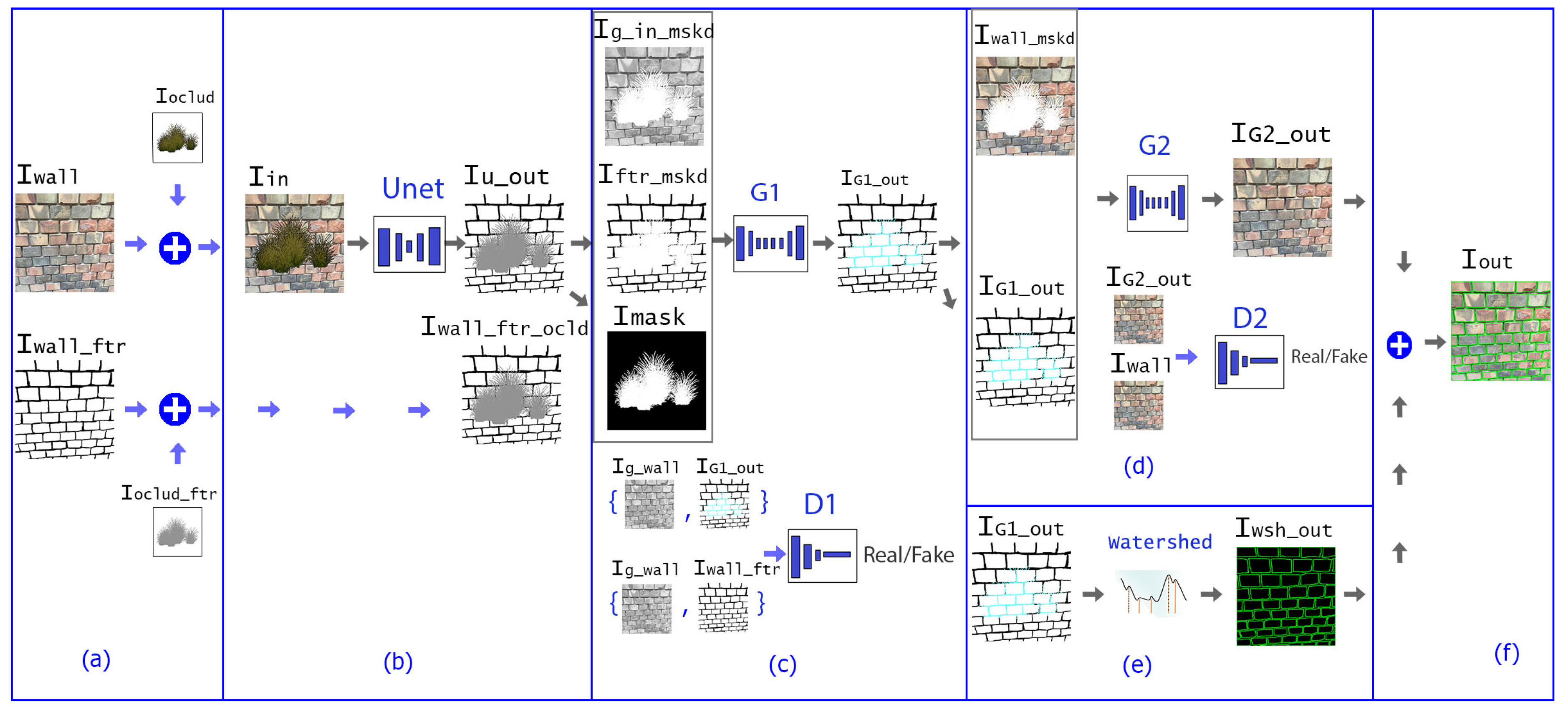
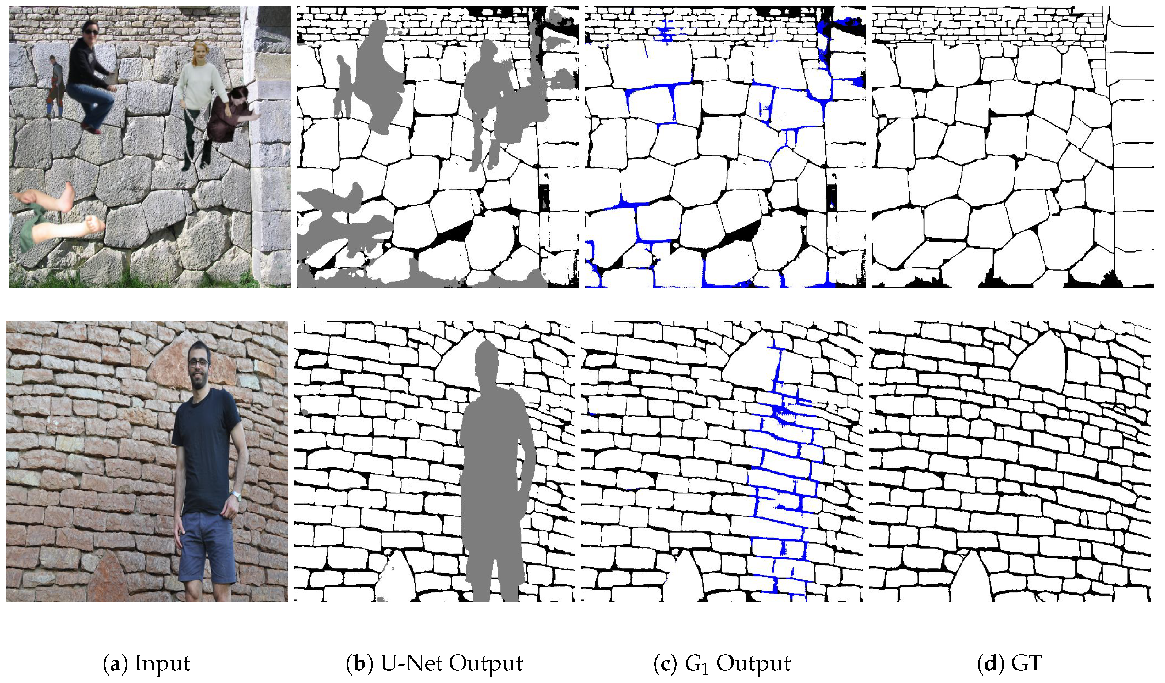
Table 1.
Evaluation of occlusion mask extraction in the Pre-processing Stage for Test Set (1) and (2).
Table 1.
Evaluation of occlusion mask extraction in the Pre-processing Stage for Test Set (1) and (2).
| Test Set | Num. of Obj. | Precision | Recall | -Score |
|---|---|---|---|---|
| (1)—Synthetic | one | 52.84 | 83.90 | 58.99 |
| two | 70.15 | 88.38 | 75.06 | |
| three | 77.36 | 89.58 | 81.49 | |
| four | 80.51 | 89.48 | 83.38 | |
| five | 83.93 | 89.71 | 85.88 | |
| average | 72.95 | 88.22 | 76.96 | |
| (2)—Real | - | 78.32 | 92.87 | 83.63 |
Table 2.
Comparison of our inpainting results to three state-of-the-art non-blind inpainting algorithms. Notation: ↑ Higher is better. ↓ Lower is better.
Table 2.
Comparison of our inpainting results to three state-of-the-art non-blind inpainting algorithms. Notation: ↑ Higher is better. ↓ Lower is better.
| Metrics | Mask | GMCNN [38] | Pluralistic [40] | EdgeConnect [42] | Our | |
|---|---|---|---|---|---|---|
| PSNR ↑ | 0–10% | 23.59 | 25.88 | 32.19 | 31.62 | |
| 10–20% | 22.25 | 23.92 | 27.73 | 27.16 | ||
| 20–30% | 21.08 | 22.38 | 24.95 | 24.34 | ||
| 30–40% | 20.11 | 21.23 | 23.09 | 22.46 | ||
| 40–50% | 19.26 | 20.19 | 21.50 | 20.91 | ||
| SSIM ↑ | 0–10% | 82.01 | 86.81 | 96.62 | 96.25 | |
| 10–20% | 75.46 | 79.73 | 91.41 | 90.52 | ||
| 20–30% | 67.73 | 71.26 | 84.01 | 82.46 | ||
| 30–40% | 60.03 | 62.48 | 75.29 | 73.44 | ||
| 40–50% | 50.98 | 51.85 | 64.72 | 62.20 | ||
| L1 ↓ | 0–10% | 5.12 | 3.61 | 0.56 | 0.57 | |
| 10–20% | 5.77 | 4.34 | 1.33 | 1.37 | ||
| 20–30% | 6.58 | 5.20 | 2.39 | 2.47 | ||
| 30–40% | 7.37 | 6.03 | 3.49 | 3.59 | ||
| 40–50% | 8.25 | 7.00 | 4.73 | 4.91 | ||
| FID-score ↓ | 0–10% | 66.65 | 43.51 | 8.88 | 8.42 | |
| 10–20% | 84.69 | 56.23 | 21.56 | 21.49 | ||
| 20–30% | 107.64 | 75.90 | 42.32 | 41.87 | ||
| 30–40% | 134.82 | 87.23 | 62.89 | 60.68 | ||
| 40–50% | 157.12 | 108.58 | 88.10 | 86.20 |
Table 3.
Evaluation of brick segmentation. Object and pixel level precision, recall, F1-score and IOU values for the Test Set (1) using different numbers (0–5) of synthetic occluding objects; and results on Test Set (2) with real occlusions.
Table 3.
Evaluation of brick segmentation. Object and pixel level precision, recall, F1-score and IOU values for the Test Set (1) using different numbers (0–5) of synthetic occluding objects; and results on Test Set (2) with real occlusions.
| Test Set | Num. of Obj. | Recall (%) | Precision (%) | F1-Score (%) | IOU (%) | |||
|---|---|---|---|---|---|---|---|---|
| Brick | Pixel | Brick | Pixel | Birck | Pixel | Pixel | ||
| (1)—synthetic | no occlusion | 82.79 | 76.58 | 73.11 | 85.14 | 76.62 | 78.20 | 70.24 |
| one | 83.85 | 76.54 | 73.39 | 85.42 | 77.25 | 78.14 | 70.49 | |
| two | 82.89 | 76.11 | 72.91 | 85.12 | 76.56 | 77.70 | 69.54 | |
| three | 83.35 | 76.20 | 73.08 | 85.27 | 76.84 | 77.84 | 69.19 | |
| four | 82.28 | 75.15 | 71.65 | 84.15 | 75.63 | 77.00 | 68.21 | |
| five | 81.47 | 74.69 | 71.93 | 82.85 | 75.47 | 76.26 | 67.01 | |
| (2)—real | no occl. | 79.76 | 72.78 | 70.73 | 80.57 | 74.44 | 74.18 | 63.78 |
| with Obj | 67.56 | 66.25 | 72.26 | 71.84 | 69.22 | 67.44 | 54.04 | |
Publisher’s Note: MDPI stays neutral with regard to jurisdictional claims in published maps and institutional affiliations. |
© 2020 by the authors. Licensee MDPI, Basel, Switzerland. This article is an open access article distributed under the terms and conditions of the Creative Commons Attribution (CC BY) license (http://creativecommons.org/licenses/by/4.0/).
Share and Cite
MDPI and ACS Style
Ibrahim, Y.; Nagy, B.; Benedek, C. Deep Learning-Based Masonry Wall Image Analysis. Remote Sens. 2020, 12, 3918. https://doi.org/10.3390/rs12233918
AMA Style
Ibrahim Y, Nagy B, Benedek C. Deep Learning-Based Masonry Wall Image Analysis. Remote Sensing. 2020; 12(23):3918. https://doi.org/10.3390/rs12233918
Chicago/Turabian StyleIbrahim, Yahya, Balázs Nagy, and Csaba Benedek. 2020. "Deep Learning-Based Masonry Wall Image Analysis" Remote Sensing 12, no. 23: 3918. https://doi.org/10.3390/rs12233918
Note that from the first issue of 2016, this journal uses article numbers instead of page numbers. See further details here.