The Met Office Operational Soil Moisture Analysis System


1
Met Office, FitzRoy Road, Exeter, Devon EX1 3PB, UK
2
MetOffice@Reading, Meteorology Building, University of Reading, Reading, Berkshire RG6 6BB, UK
*
Author to whom correspondence should be addressed.
Remote Sens. 2020, 12(22), 3691; https://doi.org/10.3390/rs12223691
Submission received: 30 September 2020
/
Revised: 6 November 2020
/
Accepted: 9 November 2020
/
Published: 11 November 2020
(This article belongs to the Special Issue Remote Sensing of Land Surface and Earth System Modelling)
Abstract
:In this study, the current Met Office operational land surface data assimilation system used to produce soil moisture analyses is presented. The main aim of including Land Surface Data Assimilation (LSDA) in both the global and regional systems is to improve forecasts of surface air temperature and humidity. Results from trials assimilating pseudo-observations of 1.5 m air temperature and specific humidity and satellite-derived soil wetness (ASCAT) observations are analysed. The pre-processing of all the observations is described, including the definition and construction of the pseudo-observations. The benefits of using both observations together to produce improved forecasts of surface air temperature and humidity are outlined both in the winter and summer seasons. The benefits of using active LSDA are quantified by the root mean squared error, which is computed using both surface observations and European Centre for Medium-Range Weather Forecasts (ECMWF) analyses as truth. For the global model trials, results are presented separately for the Northern (NH) and Southern (SH) hemispheres. When compared against ground-truth, LSDA in winter NH appears neutral, but in the SH it is the assimilation of ASCAT that contributes to approximately a 2% improvement in temperatures at lead times beyond 48 h. In NH summer, the ASCAT soil wetness observations degrade the forecasts against observations by about 1%, but including the screen level pseudo-observations provides a compensating benefit. In contrast, in the SH, the positive effect comes from including the ASCAT soil wetness observations, and when both observations types are assimilated there is a compensating effect. Finally, we demonstrate substantial improvements to hydrological prediction when using land surface data assimilation in the regional model. Using the Nash-Sutcliffe Efficiency (NSE) metric as an aggregated measure of river flow simulation skill relative to observations, we find that NSE was improved at 106 of 143 UK river gauge locations considered after LSDA was introduced. The number of gauge comparisons where NSE exceeded 0.5 is also increased from 17 to 28 with LSDA.
1. Introduction
The Met Office assimilates observations of the land surface in order to improve the set of initial conditions for numerical weather prediction (NWP). The expected benefit to NWP of including land surface information by assimilation of soil moisture observations is in the improvements to forecasts of the screen level or near-surface air temperature and humidity [1]. Surface soil moisture directly affects the latent and sensible heat fluxes at the land-atmosphere interface. Evaporation of moisture from the soil itself and transpiration from vegetation affect how energy is partitioned between the two heat fluxes. It follows that the accurate initial soil moisture state will produce more accurate estimates of the air temperature and humidity near the surface [2,3]. In this paper, we focus on soil moisture only, and not, e.g., on snow cover or soil temperature, which are also important components of the land surface system.
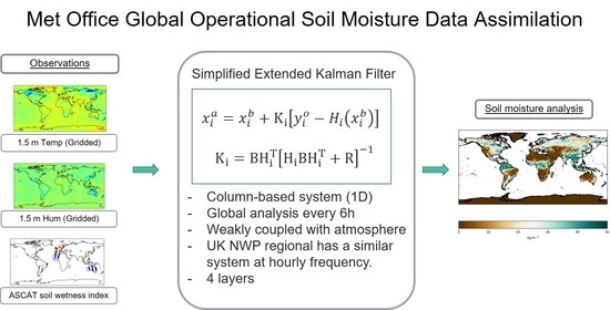
The Met Office operational assimilation scheme has included data relevant to the land surface since August 2005. The first method used was a land surface nudging scheme [4,5]. This was an effective method to constrain the soil moisture using air temperature and relative humidity measurements but was difficult to extend to incorporate other observation types. Consequently, the Simplified Extended Kalman Filter [6] was subsequently adopted in early 2013. Land surface data assimilation (LSDA) at the Met Office was exclusive to the global model until 2019. Before then, the UK regional model, a convection-permitting, 1.5 km numerical weather prediction (NWP) model called the “UKV” [7], received a daily update of an interpolated soil moisture analysis from the global model. In December 2019, an hourly-cycling, regional land surface data assimilation system, based on the global system approach, became operational.
The observations assimilated include pseudo-observations of 1.5 m air temperature and specific humidity constructed via the Met Office atmospheric DA system and remotely-sensed soil wetness derived from the surface backscatter measured by scatterometers (ASCAT) aboard the MetOp series of satellites [8]. These ASCAT observations are delivered in near real time to the Met Office by the European Organisation for the Exploitation of Meteorological Satellites (EUMETSAT). The feasibility of assimilating pseudo-observations of screen temperature and humidity to initialise soil moisture conditions for NWP was first demonstrated by [9]. It has become a standard and highly practical method used at many national meteorological centres. The use of the ASCAT soil wetness product in the land surface data assimilation system in the global Met Office NWP system was presented by [10].
The goal of this work is to introduce the operational LSDA system at the Met Office and illustrate its application in both the global and regional operational modelling systems. Following the classification in [11,12] both global and UKV LSDA systems are weakly coupled to the atmospheric DA system, which indicates that both analyses are independent but the models representing each earth system component (i.e., atmospheric and land) are fully coupled in the forecast step. To our knowledge, the Met Office has operationally implemented the first regional weakly coupled LSDA system. The benefits of regional-scale assimilation beyond its impact in the NWP system has been explored through evaluation of simulated river flow against observations. This emphasises the importance of a well-represented hydrological state in order to realise the potential for more integrated hydro-meteorological predictions [13,14,15,16].
2. Materials and Methods
Land surface data assimilation is accomplished by using an algorithm to combine the output of a land surface model and observations of the land surface to obtain an “analysis” that is used to initiate an NWP model. A forecast made using the analysis as initial conditions should compare more favourably to independent observations than a forecast made using the same model with “first guess” or uncorrected initial conditions to predict those variables. At present, there is a large selection of land surface models and numerous land surface observations that can be used.
Apart from a choice in algorithm to implement the land surface DA, there is a variety of land surface models that can be used to couple the land and atmosphere within a modelling system. The Joint UK Land Environment Simulator (JULES) [17] is the land surface model used operationally at the Met Office and the one used in this study. At the European Centre for Medium-range Weather Forecasts (ECMWF), the model “Hydrology Tiled ECMWF Scheme for Surface Exchange over Land” (H-TESSEL) [18] is used. At Environment Canada they use the “Soil, Vegetation and Snow” (SVS) [19] land surface model. The North American community model “Noah” [20,21] is in use at the National Center of Environmental Prediction (NCEP). Meteo-France developed the Interaction Sol-Biosphere-Atmosphere (ISBA) [22,23].
Choices of observations to assimilate have been somewhat limited until recently, for various reasons. There are in situ observations of soil moisture and satellite soil moisture or wetness products, which are the result of careful retrievals from either backscatter (active instruments) or radiance (passive instruments) measurements. Soil moisture observations are difficult to interpret for several reasons. Firstly, in situ observations are truly a point source observation of a very specific soil (texture, porosity) that may not be reflected in the assumptions that an NWP model makes at a grid point about land cover and soil composition. In reality, soil is a very heterogenous medium; therefore, an in situ measurement not made at a site chosen for its highly uniform land cover is difficult to interpret more widely. Soil moisture products derived from satellite-based remote sensing, such as ASCAT soil wetness, have spatial resolutions typically in the range of 1 to 50 km, depending on the measurement frequencies employed. Therefore, they represent a wider region than in situ data and consequently are closer to the spatial scales modelled in global and regional NWP schemes.
2.1. Land Surface Data Assimilation Algorithm
Land analysis is a 1D system calculated independently for each soil column. This is based on the assumption that the horizontal fluxes are much slower than the vertical and therefore they can be neglected in the timescales the analysis is applied. We compute our analysis using a Simplified Extended Kalman Filter (SEKF) algorithm [24], which is expressed by the equation:
At an i-th grid point, x represents the land model state, superscripts a and b indicate analysis and background respectively, y is the observation vector and ℌ denotes the non-linear observation operator that projects the model values into the observation space. The background is provided by the forecast from the operational model run from the previous cycle, which is 6 h before the global analysis time and 1 h before the UKV analysis time. K, also known as the Kalman Gain, is a matrix with the weights of the linear combination between observation values and model values and is expressed as:
where B and R are the background and observation error covariance matrices and H is a linear observation operator expressed in matrix form calculated through a Jacobian estimation, which we describe at Section 2.2. Error covariances between soil layers are ignored and the diagonal is set in terms of the standard deviation as σB = 0.030, 0.026, 0.026, 0.026 m3/m3, values are the same for all soil points. The B-matrix values have been estimated using a triple collocation method comparing the model background against two independent observational sources: SMOS satellite soil moisture product [25] and around 200 soil moisture in-situ observations from networks located in US, France, and Australia [26,27]. See Section 2.2 and Section 2.3 for a description of the R values.
2.2. Jacobian Method
The linear observation operator H at (2) is approximated by the first derivative (i.e., Jacobians). This is estimated by running a set of JULES standalone runs, a control run, and a perturbed run for each analysis variable initialised by applying a small perturbation at the initial conditions. Each of the positions of the H matrix are expressed by:
where n denotes the n-th control variable and m is the m-th observation variable, is the perturbation at the beginning of the forecast and Hm(xt2) denotes the model state converted to an observation quantity m at the end of the forecast, superscripts c and p represent the control and perturbed runs. The initial perturbation and the length of the forecast need to be small enough to preserve the linear approximation but large enough to capture the sensitivity across variables. The length of the forecast is chosen to be 3 h for the global model and 1 h for the regional UKV, while the initial perturbation is set to a value of 0.005 m3/m3. By using an estimated Jacobian we can include information of the errors of the day in the Kalman Gain calculation (2). The B matrix is diagonal and homogenous; therefore, including information at each grid point related to the flow regime is beneficial.
2.3. Assimilation of Atmospheric Surface Observations
Though not technically land surface variables, the atmospheric screen level (1.5 m above surface) temperature and humidity are strongly coupled to the surface soil moisture [28]. Brubaker, K.L. et al. [29] developed a conceptual slab model of the moisture and energy in a surface soil layer coupled to the atmospheric boundary layer. They presented an equilibrium solution to their simple model to demonstrate how in continental climates, the amount of moisture in the surface soil layer affects the partitioning of the latent and sensible heat fluxes. Thus, the physics of the interface mean that it is permissible to use so-called pseudo-observations (produced via a pre-processing step that interpolates the observations to the model grid points) of the near-surface air temperature and humidity to adjust the model surface soil moisture.
Drusch, M. et al. [30] tested the use of pseudo-observations in a land surface data assimilation system. In a Northern hemisphere summer they found that the turbulent surface fluxes were better forecast, and, consequently, the weather forecast over large areas was improved as verified by the temperature at three atmospheric pressure levels. However, the soil moisture profiles themselves, when compared to in situ network measurements, were not improved to the point where they were useful for hydrological or agricultural models. They concluded that because the soil moisture analysis was determined via assimilation of the pseudo-observations and not by a direct observation of soil moisture, that the “soil moisture is a sink variable in which errors introduced through the atmospheric forcings and the land surface model accumulate.” [30]. Their study is a motivating factor for the manner in which experiments are set up in this demonstration of the Met Office system.
Directly ingesting near surface in-situ observations has limitations, as they are typically not sufficiently dense to cover all grid points in the model domain. Since the lateral processes in soil are typically slower than vertical movements, there is a risk of introducing climate islands at the grid points where observations are available. It is common to use a technique where observations are first interpolated to all model grid points and then ingested as pseudo-observations (i.e., they are treated as observations in every sense by the data assimilation algorithm).
In the global system, we generate our pseudo-observations by ingesting the in-situ observations in the Met Office atmospheric data assimilation software (VAR) using a 3D-Var algorithm [31] that uses the atmospheric model as the background. Model and observation error covariances are the same as in the operational model. Since we are using the resulting atmospheric analysis at the lowest level as our pseudo-observations, we can see that:
where uppercase A and L refer to the atmospheric and land models, respectively. Because the UM atmosphere and JULES land surface models are fully coupled, the atmospheric model background is equivalent to the land background projected to the atmosphere space.
Combining Equations (4) and (5), we find that the atmospheric analysis increment is equivalent to the land innovation:
The VAR system provides atmospheric analysis increments at lowest model level (currently a height of 20 m above ground level in the global and 5 m in the UKV). We assume that these are valid at 1.5 m, and we ingest the analysis increments as innovations in (1). In the UKV we extend (6) by ingesting the increments from the atmospheric analysis described by [32], effectively increasing the interaction between the atmospheric and land analysis DA systems. The R-matrix is diagonal, and the observation error is expressed in terms of the error variance. The terms are set to the same value used for screen temperature and humidity observations in the atmospheric DA system; that is 1.5 K and 8% for the global, and 0.8 K and 5% for the UKV.
Weakly Coupled vs. Quasi-Strongly Coupled
Some information from the atmospheric analysis is used in the land analysis through the ingestion of screen observations (global) or the analysis itself (UKV), which is one of the requirements of a quasi-strongly coupled system. However, the opposite is not true, and the only feedback from the land analysis into the atmospheric analysis is through the coupled model run. Because the interaction between the analyses is one-way, it seems appropriate to follow a conservative approach and label our system as weakly coupled.
2.4. Assimilation of ASCAT Soil Wetness
Observations of surface soil wetness taken from the Advanced SCATterometer (ASCAT) L2 product are assimilated. This product is derived from backscatter measured by the same instrument on the three Meteorological Operational satellite platforms: MetOp-A, MetOp-B, and MetOp-C [8,33,34]. Note that the data from satellite MetOp-C was not used operationally at the Met Office for the time periods of the trials considered in this work, because MetOp-C was launched on 7 November 2018. This soil wetness product only represents the soil moisture in the first few cm of soil, but this is taken into account by matching it to the model soil wetness in the top layer (10 cm) via a bias correction [10].
ASCAT has been chosen over other satellite-based products because it has characteristics that make it more suitable for NWP applications. It is delivered in a timely way so that NWP forecasts can be produced in real time; this is a critical feature of any data stream used in an operational NWP system at a National Meteorological Service. The scatterometer instrument is on board three different satellites: MetOp-A, -B, and the new –C, which together provide a data stream with excellent resilience and global coverage. The soil wetness retrieved from the measured backscatter is based on a relatively simple rescaling algorithm which, unlike other soil moisture products, does not involve a retrieval scheme that includes strong assumptions about the land surface (e.g., soil type), making it less likely to have additional biases. That being said, the relatively shorter wavelengths employed by the ASCAT instrument means that some regions are not usable, e.g., over dense forest. One of the strengths of the EKF approach is that we can combine soil moisture information from several different sources of observations. It is hoped in the future that other satellite products can be assimilated.
Quality control is performed by rejecting ASCAT soil wetness data where there is snow cover, frozen soil, wetlands or mountains, where the estimated error is too large and for pre-determined cross track cell numbers. Once the observations have gone through this preliminary quality control, they can be transformed to the model grid.
The model and the observations are on different latitude and longitude grids. They also represent different spatial resolutions. Observations are mapped to the model grid using an inverse distance weighting interpolation algorithm [35]. A modification to the standard global search was implemented via a neighborhood search in order to improve computational performance (see Appendix A description of the algorithm).
In the Met Office LSDA system, the observations of soil moisture are converted from soil wetness index to the volumetric soil moisture. It is necessary to bias correct the observations before assimilation so that the model and observational climates match [36]. This can be done in a number of ways, including a technique known as Cumulative Distribution Function matching [37]. At the Met Office, the current operational system implements the bias correction by taking a fraction of the ASCAT soil wetness anomaly (from its observational climate) and adding it to the model’s monthly mean surface soil moisture. Thus, the observation is used to modify the model climatology and it is this value that is then assimilated. Details can be found in [10]. The UKV domain climatology is derived from the global climatology by converting the soil moisture into vegetation stress [17] using the global soil properties, interpolating it to the UKV grid, and then converting it back to soil moisture using the UKV soil properties. After the ASCAT surface soil wetness is converted to volumetric soil moisture and re-gridded as described above, there is another quality control performed using the model background. Observations are rejected if the probability of gross error exceeds 50%. This probability is computed for each observation and its corresponding background value according to the theory laid out in [38], which assumes that the errors are Gaussian distributed and that the background and observation errors are uncorrelated. ASCAT observation error is specified in terms of the error variance and is set to 0.035 m3/m3. The value has been calculated using the departures of the observations from the background and the observations from the analysis, as described in [39].
2.5. Description of the System
The impact of LSDA is assessed by running a series of experiments in both global and regional atmospheric model configurations. The global model is the Met Office Unified Model (UM) [40] based on the Met Office Operational Suite 42 (OS42, operational between March and December 2019), which uses the UM with Global Atmosphere 6.1 configuration [41] coupled to JULES with Global Land 8.1 configuration [17]. Initial atmospheric conditions are provided by the Met Office Hybrid 4D-Var data assimilation system [42]. The operational global NWP system runs at a grid resolution of N1280 (approximately 10 km at mid-latitudes) which is computationally too expensive to run our tests (Figure 1a), so instead we have used N320 resolution (approximately 40 km at mid-latitudes) which is the standard Met Office resolution to evaluate improvements. Similarly, to avoid running an ensemble alongside the deterministic forecast, the errors-of-the-day part of the error covariance is taken from the operational ensemble and interpolated to the analysis grid. Global forecasts are run for six days with a cycling frequency of 6 h. The regional model, or UKV, is centred on the British Isles (Figure 1b) with a horizontal resolution of 1.5 km in the interior of the domain and 4 km at the borders, initial conditions are provided by a Hybrid 4D-Var data assimilation system. Details about data assimilation as well as the atmospheric and land scientific configuration are described by [32]. UKV forecasts have an hourly cycling frequency where the runs initialised at 00Z, 06Z, 12Z, and 18Z are run for 1.5 days and the rest for 3 h.
NWP improvements are typically presented as incremental changes over the previous operational suite. LSDA has been in the global NWP system for several years so it is not possible for us to show the comparison with the previous system. To illustrate the impact of LSDA, we run a set of sensitivity experiments where our control, which is labelled free-run, features no land data assimilation and the soil moisture fields are passed from one cycle to the next allowing the soil moisture field to evolve without constraint. The impact of the individual observation types is assessed by running experiments LSDA-S and LSDA-A, which ingest only screen observations and ASCAT, respectively. Our operational system, which ingests both observations, is presented as LSDA-O. The regional system in OS42 does not include LSDA and the initialisation of soil moisture is performed by replacing the soil moisture fields with an interpolation of the soil moisture analysis from the global model at the 09Z cycle. In the UKV experiments, we include an additional set-up, labelled daily-update, which represents this scientific configuration to show the impact of adding LSDA to the operational system. Experiments are summarized in Table 1.
For our experiments, we follow the standard evaluation procedure at the Met Office for testing operational changes. We run two testing periods starting 1 December 2017 and 1 July 2017, which correspond to the Northern hemisphere winter and summer, respectively. The global trials are run for three months and the UKV trials for two months; this should ensure statistical robustness in our results and avoid sampling the same synoptic structures across the domain. This is particularly relevant in the global model, which contains several climates at the same time, and is why the experiment length is chosen to be longer. Both systems are initialized from the global operational analysis that is closest to the start of each trial period and all UKV experiments are driven by the global LSDA-O run; hence, the only differences are related to the LSDA changes. Results are compared to SYNOP observations using the Met Office standard verification system.
3. Results and Discussion
3.1. Global Model
Results for experiments during the winter and summer trial periods are presented in terms of root mean squared error (RMSE) of the forecasts of 1.5 m air temperature (K) as a function of forecast lead times for the Northern and Southern hemispheres. Alongside the 1.5 m relative humidity (not shown), the 1.5 m temperature fields are one of the most important to users of forecasts made at an operational centre. Therefore, developments which successfully improve or create the pathway for improvements in these fields are important. The experimental forecasts are compared to SYNOP surface observations in Figure 2 and Figure 3 and to the global analysis fields provided by ECMWF analysis in Figure 4 and Figure 5.
3.1.1. Comparison against Observations
In winter, in Figure 2a, the Northern Hemisphere RMSE differences between all of the experiments and control appear neutral and this is confirmed by Figure 2b, which for all experiments shows less than 1% difference from the free-run (red). For the Southern hemisphere winter, Figure 2c shows that the LSDA-S experiment (blue) has smaller RMSE than the free-run for lead times less than 48 h and LSDA-A (green) has larger RMSE than the free-run. Together in LSDA-O (pink), the two observation types provide a neutral result and beyond 48 h it is the LSDA-A which contributes to the improvement in the LSDA-O. This is seen more clearly in Figure 2d where the first 48 h of the forecasts appear neutral as in the Northern hemisphere, but beyond this lead time, both LSDA-A and LSDA-O improve the comparison with respect to the SYNOP observations by about 1%. Indeed, we expect to see neutral results in the Northern hemisphere winter due to the presence of snow cover and frozen soil, where the quality control sets the soil moisture increments to zero.
In the Northern hemisphere summer, Figure 3, panels a and b, show that including the screen level pseudo-observations in LSDA-S improves the forecast slightly but including the ASCAT soil wetness observations (LSDA-A) degrades the forecasts against observations by about 1%. When both observations types are used (LSDA-O), there is a compensating positive effect from including the screen observations and the total effect is neutral. In contrast, in the Southern hemisphere summer Figure 3 panels c and d show a small, but positive, effect from including the ASCAT soil wetness observations. Thus, in the Southern hemisphere, while the overall result (LSDA-O) is neutral again, the effect of including each observation type is reversed.
3.1.2. Comparison against ECMWF Analysis
The comparison to the ECMWF analysis fields [43] of 1.5 m air temperatures (K) is another measure of the Met Office system independent of its own analysis. Figure 4 shows that adding LSDA using either or both types of observations for both hemispheres in winter gives a small improvement in terms of RMSE. We conclude that, in winter, the LSDA-O has a neutral impact on the system when measured against the ECMWF analysis field.
Figure 5a,b shows that in the Northern Hemisphere summer period, LSDA-A degrades the forecast slightly when compared to LSDA-S, but in the experiment including both observations (LSDA-O) the result is neutral at all lead times. In the Southern hemisphere, Figure 5c,d shows that LSDA-A provides a benefit to the forecasts.
3.1.3. Conclusions about Global LSDA Performance
By comparing the Met Office forecasts over the course of a winter season with both observations and an independent analysis of the 1.5 m air temperature fields, we conclude that the LSDA-S, LSDA-A, and LSDA-O experiments show a neutral to positive impact in both hemispheres.
In the summer, in the Northern hemisphere, there are indications that the assimilation of ASCAT soil wetness observations in LSDA-A slightly degrades the system. There are small, but negative, results in RMSE when compared against the SYNOP observations and the ECMWF analyses. However, in the Southern hemisphere, the LSDA-A adds a clear benefit. This contrast has led the Met Office to investigate the bias correction procedures used in the assimilation of ASCAT soil wetness observations. Results from that will be published in a future study. Finally, the improvement in screen humidity (not shown) suggests that the soil moisture analyses are contributing to improvements in the latent heat fluxes at the surface. Changes in soil moisture can potentially affect the mass fluxes and lead to changes in precipitation. However, our verification for this variable showed no impacts at all lead times and areas, suggesting that the precipitation patterns have not been significantly altered in the experiments. Verification for other relevant variables, such as wind and pressure, also showed neutral results.
3.2. UKV Regional Model LSDA
Results for the same seasons used for the global are presented, but only for a shorter period. In addition to RMSE against surface observations for temperature, we also include relative humidity in our discussion. We use the same experiment configurations as in the global plus an additional set-up, labelled daily-update, which represents the OS42 operational configuration. Comparisons between daily-update and LSDA-O demonstrate the impact of adding the regional LSDA system to the Met Office operational system.
3.2.1. Comparisons against Surface Observations
Verification results for 1.5 m temperature and humidity for winter and summer periods are shown in Figure 6 and Figure 7 respectively. RMSE for winter temperature (Figure 6a) shows a neutral impact at all lead times for all experiments. Difference against control (Figure 6b) shows that all experiments with LSDA have an increase in RMSE that grows with lead time and is around 1% at the end of the forecast. Daily-update shows a lower overall error than experiments with LSDA with a similar performance to free-run. Relative humidity RMSE (Figure 6c) shows no significant impact from any of the experiments and the difference against control (Figure 6d) suggests no meaningful trend.
In summer (Figure 7a), applying different LSDA configurations indicates a larger impact in the RMSE than winter (Figure 6a), reflecting the fact that in winter a larger area of soil is frozen or covered in snow. LSDA-O, daily-update, and LSDA-A show a degradation with respect to control, particularly at the early hours of the forecast—the latter being the poorest performer. LSDA-S shows a consistent improvement for all lead times, suggesting that assimilating surface observation provides useful information. The benefits can be seen in the LSDA-O experiment as its RMSE is lower than LSDA-A. RMSE for relative humidity (Figure 7c,d) shows a positive impact from all experiments with respect to free-run, with LSDA-O showing the largest improvements. The experiments that assimilate a single observation type both offer improvements—LSDA-A being the best of the two. Daily-update still improves on the free-run, but not as much as when a regional data assimilation system is used (LSDA-O).
3.2.2. Conclusions about UKV LSDA
Comparisons against RMSE show that the impact of including LSDA with respect to the free-run is limited, particularly in winter. Results for the summer period show that the temperature is slightly degraded and relative humidity is improved. The two observation types have different contributions, while LSDA-S gives the best results for temperature, LSDA-A is the main contributor to lower RMSE for relative humidity. The comparison against daily-update provides a measure of the improvement in these two fields from the OS42 to OS43 operational upgrade of the LSDA system. The performance in temperature is comparable between daily-update and LSDA-O while the relative humidity forecast is improved from daily-update to LSDA-O. It should be noted that daily-update replaces the entire soil column with a new soil moisture profile once a day. This has a significant limitation, as it does not allow the system to evolve to its own climate and significantly constrains the potential for regional-scale land model research and improvements. Despite LSDA-O not being substantially better than daily-update in terms of surface verification, it provides a system with comparable regional NWP. Similar to what was observed in the global, verification for precipitation (and other variables) show no significant impact.
3.3. Regional LSDA Impact on Runoff and River Flow Prediction
The previous results were focused on assessment of system performance relative to near-surface meteorological variables, using verification tools typical of that used to help assess model upgrades for most operational NWP centres. While improving NWP performance is a clear requirement for any LSDA implementation, this approach does not provide any insight as to the impact of changes on the hydrological state of the system. In order to consider this using independent observations, the impact of the regional LSDA on river flow simulations was assessed. To summarise the impact of the LSDA-O implementation, a comparison is presented using hourly analyses of the OS42 operational system and from the parallel suite PS43 regional candidate that included the LSDA-O configuration running between mid-July and the start of December 2019. The surface and sub-surface runoff diagnostics were extracted for each system and used as input to an offline implementation of the JULES river routing scheme with a 30 min routing timestep and default flow parameters [44,45].
Observations from 139 of the UK National River Flow Archive (NRFA) Benchmark Network [46] subset of UK river flow gauges were used for this assessment as these are considered relatively free from anthropogenic influence and more suitable for characterising hydrological variability. The full data are released annually, and are available for all gauges up to the end of September 2019 only. This covers a relatively low flow period at the start of the OS42/PS42 assessment period. For 58 of these gauge locations, raw data from the Environment Agency data feed [47] was therefore used to assess the full period instead. For simplicity here, the hydrological simulation performance is assessed in terms of Nash-Sutcliffe Efficiency (NSE; [48]).
Figure 8a shows an illustrative time series at the Haw Bridge gauge location on the River Severn in southern England (marked in Figure 8b) of observed and simulated river flows using the OS42 (equivalent to daily-update) and PS43 (equivalent to LSDA-O) runoff inputs. There is a clear improvement to the simulated flows using the new system PS43 inputs relative to OS42. In this case, NSE for the OS42 input time series is less than -1, noting that a value less than zero indicates that the observed mean flow would be a better predictor that the simulation. By contrast, the PS43 result of 0.75 is comparable to other hydrological models and optimised JULES results previously obtained driven by an observations-based forcing [45]. In common with results at many other gauge locations, this can be attributed to a much-improved representation of the sub-surface runoff in PS43 relative to OS42. The OS42 (daily-update) system has unrealistically large soil moisture increments in lower levels, which leads to unrealistically high river flow predictions across much of the UK. This is substantially improved when simulating river flows from PS43 input runoffs (Figure 9b).
Results for all available gauge locations are summarised in Figure 9. This highlights the overall improvement to river flow predictions using PS43. NSE metrics were improved for PS43 relative to OS42 at 106 of 143 gauge locations, and values in excess of 0.5 were obtained for 28 gauges for PS43 compared to 17 gauges using OS42 inputs (noting that not all gauges have observations reported for the full assessment period). Where OS42 results are better than PS43, these generally occur where NSE from both simulations are well below zero and associated with generally low flow regions. Figure 9b highlights improved statistics that were generally obtained for catchments with larger flow volumes, and results are generally noisy where observed flows were closer to zero.
Note this analysis has not included any tuning or calibration of the river flow simulation, as the emphasis is to understand the impact of the adjustment to soil moisture state on river flow as a diagnostic metric. However, these results clearly highlight that the new regional LSDA brings substantial benefit for hydrological performance and offers the prospect for provision of a more integrated approach to hydro-meteorological prediction at regional scales in future.
4. Conclusions
The operational soil moisture LSDA system at the Met Office has been described for both global and regional applications. We use a Simplified Extended Kalman Filter and ingest pseudo-observations of screen temperature and humidity and satellite-derived soil wetness (ASCAT). The processing of observations in terms of quality control, interpolation, and bias correction is described for both observation types.
For the global model, a set of experiments is presented to assess the impact of LSDA in the overall performance of the NWP system. For this we run trials for two seasons, winter and summer, and assess the results against two truth types using the root mean squared error. Results show that LSDA provides an overall positive impact across hemispheres and seasons. Evaluation of the impact of the different observation types shows that their positive contribution depends on the area and season. Thus, assimilating both types provides a complementary combined benefit.
For the Regional model or UKV, a similar set of experiments is presented, where an additional benchmark of the previous operational regional NWP system is included. Comparison against 1.5 m observations of temperature and humidity shows that LSDA provides a neutral impact over winter and a mixed result for summer, where temperature is degraded, and specific humidity is improved when compared to the free-run. However, when using the previous operational system as a benchmark (daily-update) the performance in temperature is comparable and the humidity is improved. Similar to what was observed in the global, the combined use of both observations provides individual relevant contributions to the overall performance of LSDA-O. Comparing river flow predictions forced with output from the previous operational regional NWP system and the new LSDA outputs highlights a substantial improvement in the hydrological state and extends the assessment of the LSDA system beyond more traditional NWP-focused metrics. Such assessments should become a more integral part of operational system monitoring. This work also highlights that regional NWP with LSDA can provide useful hydrological information from an integrated and self-consistent atmosphere-land system. These results deemed LSDA-O as acceptable for inclusion in operations as of December 2019, opening the door for land modellers to evaluate and improve the physical behaviour of JULES, and bringing the potential to include future improvements within the LSDA scheme by improving the algorithm or including more observations.
The Met Office will continue to develop its LSDA systems in the future. First, we will investigate the current method for ASCAT bias correction and its role in the performance of the Global and UKV systems, particularly in summer. Next, we plan to expand the analysis vector to include more land variables, such as soil temperature and skin temperature. A more complete analysis vector has the potential benefit of providing consistent analysis increments across the land state. To this end, land surface temperature is becoming an observation type of great interest for NWP at the Met Office. In addition, we would like to explore satellite soil moisture observations such as the near real time neural net SMOS soil moisture product [49].
Author Contributions
Conceptualization, B.G., C.L.C.-P., H.L. and B.C.; methodology, B.G., C.L.C.-P., H.L. and B.C.; software, B.G., C.L.C.-P., H.L. and B.C.; validation, B.G., C.L.C.-P., H.L. and B.C.; formal analysis, B.G., C.L.C.-P., H.L. and B.C.; investigation, B.G., C.L.C.-P., H.L. and B.C.; data curation, B.G., C.L.C.-P. and B.C.; writing—original draft preparation, B.G., C.L.C.-P. and H.L.; writing—review and editing, B.G., C.L.C.-P., H.L. and B.C.; visualization, B.G., C.L.C.-P. and H.L. All authors have read and agreed to the published version of the manuscript.
Funding
This research received no external funding.
Acknowledgments
Keir Bovis, Imtiaz Dharssi and Bruce Macpherson for discussions on the original implementation of the EKF. David Walters and Chris Harris for discussions about operational implementation.
Conflicts of Interest
The authors declare no conflict of interest.
Appendix A. Inverse Distance Weighting Algorithm
ASCAT soil wetness observations ϕi are interpolated to points xj on the UM grid using an inverse distance weighting (IDW) interpolation algorithm [50] in Equation (A1)
where xj is the j-th target model grid point, ϕi is the i-th observation value and ri is the distance between ϕi and xj raised to the power a. Typically, the summation is performed over all observations available within a radius of influence around the model grid point to prevent the procedure from becoming too expensive computationally. We currently use 25 km as the radius of influence, which is twice the ASCAT product effective resolution. Larger values of parameter a result in observations far away having less overall impact in the summation. This exponent is a tuning parameter in our system and we currently use a = 1 for the global and a = 2 for the UKV. Distances ri are calculated using the great circle distance metric.
In order to improve computational efficiency, we have implemented a variation of the standard global search. The steps of the algorithm are outlined below.
- First, the algorithm loops through the list of observations ϕi to determine which model grid points are affected by that observation (i.e., which model grid points have that observation in their radius of influence). At each iteration, the code:
- Determines which model grid point is closest to ϕi. This can be done analytically for the global regular grid. For the UKV, ϕi is rotated to the UKV grid system of reference and the i-th and j-th positions are then found independently across x and y directions.
- Loops in a region around that model grid point and determines which model grid points in its neighbourhood are affected by the observation ϕi (i.e., are within the radius of influence).
- Stores the observation ID for ϕi at each model grid point in the neighbourhood if xj is affected by that observation; checks that the model and observation are matched only once.
- Perform the interpolation by looping through each model grid point xj. At each iteration, the code:
- Checks if xj is affected by an observation. If not, skips to next model grid point.
- If a model grid point has any observations matched with it, loops through all observations that have been matched with it during step 1.c, and calculates the two sums in Equation (A1).
As implemented in the Met Office system, this algorithm relies on the fact that it is possible to efficiently calculate which is the nearest model grid point to an observation (step 1.a). Because this is possible, the procedure can avoid performing a global search; hence, computational efficiency is significantly improved.
References
- Candy, B. Use of Satellite Information in Land Data Assimilation to Support Operational NWP; ECMWF Seminar on the Use of Satellite Observations in NWP: Reading, UK; ECMWF: Reading, UK, 2014. [Google Scholar]
- Deardorff, J.W. A Parameterization of Ground-Surface Moisture Content for Use in Atmospheric Prediction Models. J. Appl. Meteorol. 1977, 16, 1182–1185. [Google Scholar] [CrossRef]
- Deardorff, J.W. Efficient prediction of ground surface temperature and moisture, with inclusion of a layer of vegetation. J. Geophys. Res. 1978, 83, 1889. [Google Scholar] [CrossRef] [Green Version]
- Best, M.J.; Jones, C.P.; Dharssi, I.; Quaggin, R.M. A Physically Based Soil Moisture Nudging Scheme for the Global Model; Technical Report; Met Office: Exeter, UK, 2007.
- Best, M.J.; Maisey, P.E. A Physically Based Soil Moisture Nudging Scheme; Technical Report; Met Office: Exeter, UK, 2002.
- De Rosnay, P.; Drusch, M.; Vasiljevic, D.; Balsamo, G.; Albergel, C.; Isaksen, L. A simplified Extended Kalman Filter for the global operational soil moisture analysis at ECMWF. Q. J. R. Meteorol. Soc. 2013, 139, 1199–1213. [Google Scholar] [CrossRef]
- Tang, Y.; Lean, H.W.; Bornemann, J. The benefits of the Met Office variable resolution NWP model for forecasting convection. Meteorol. Appl. 2013, 20, 417–426. [Google Scholar] [CrossRef]
- Bartalis, Z. ASCAT Soil Moisture Report Series No. 15 ASCAT Soil Moisture Product Handbook; Technical Report; TU Wien: Viena, Austria, 2008. [Google Scholar]
- Mahfouf, J.-F. Analysis of Soil Moisture from Near-Surface Parameters: A Feasibility Study. J. Appl. Meteorol. 1991, 30, 1534–1547. [Google Scholar] [CrossRef] [Green Version]
- Dharssi, I.; Bovis, K.J.; Macpherson, B.; Jones, C.P. Hydrology and Earth System Sciences Operational assimilation of ASCAT surface soil wetness at the Met Office. Hydrol. Earth Syst. Sci. 2011, 15, 2729–2746. [Google Scholar] [CrossRef] [Green Version]
- Browne, P.A.; de Rosnay, P.; Zuo, H.; Bennett, A.; Dawson, A. Weakly coupled ocean-atmosphere data assimilation in the ECMWF NWP system. Remote Sens. 2019, 11, 234. [Google Scholar] [CrossRef] [Green Version]
- Penny, S.G.; Akella, S.; Alves, O.; Bishop, C.; Buehner, M.; Chevallier, M.; Counillon, F.; Draper, C.; Frolov, S.; Fujii, Y.; et al. Coupled Data Assimilation for Integrated Earth System Analysis and Prediction: Goals, Challenges and Recommendations; Technical Report; World Weather Reseach Programme: Geneva, Switzerland, 2017. [Google Scholar]
- McMillan, H.K.; Hreinsson, E.Ö.; Clark, M.P.; Singh, S.K.; Zammit, C.; Uddstrom, M.J. Operational hydrological data assimilation with the recursive ensemble Kalman filter. Hydrol. Earth Syst. Sci. 2013, 17, 21–38. [Google Scholar] [CrossRef]
- Durnford, D.; Fortin, V.; Smith, G.C.; Archambault, B.; Deacu, D.; Dupont, F.; Dyck, S.; Martinez, Y.; Klyszejko, E.; Mackay, M.; et al. Toward an operational water cycle prediction system for the great lakes and St. Lawrence river. Bull. Am. Meteorol. Soc. 2018, 99, 521–546. [Google Scholar] [CrossRef]
- Pappenberger, F.; Dutra, E.; Wetterhall, F.; Cloke, H.L. Deriving global flood hazard maps of fluvial floods through a physical model cascade. Hydrol. Earth Syst. Sci. 2012, 16, 4143–4156. [Google Scholar] [CrossRef] [Green Version]
- Thirel, G.; Martin, E.; Mahfouf, J.-F.; Massart, S.; Ricci, S.; Regimbeau, F.; Habets, F. A past discharge assimilation system for ensemble streamflow forecasts over France—Part 2: Impact on the ensemble streamflow forecasts. Hydrol. Earth Syst. Sci. 2010, 14, 1639–1653. [Google Scholar] [CrossRef] [Green Version]
- Best, M.J.; Pryor, M.; Clark, D.B.; Rooney, G.G.; Essery, R.L.H.; Ménard, C.B.; Edwards, J.M.; Hendry, M.A.; Porson, A.; Gedney, N.; et al. The Joint UK Land Environment Simulator (JULES), model description-Part 1: Energy and water fluxes. Geosci. Model Dev. 2011, 4, 677–699. [Google Scholar] [CrossRef] [Green Version]
- Balsamo, G.; Viterbo, P.; Beljaars, A.; Van Den Hurk, B.; Hirschi, M.; Betts, A.K.; Scipal, K. A Revised Hydrology for the ECMWF Model: Verification from Field Site to Terrestrial Water Storage and Impact in the Integrated Forecast System. J. Hydrometeorol. 2009, 10, 623–643. [Google Scholar] [CrossRef]
- Husain, S.Z.; Alavi, N.; Bélair, S.; Carrera, M.; Zhang, S.; Fortin, V.; Abrahamowicz, M.; Gauthier, N. The Multibudget Soil, Vegetation, and Snow (SVS) Scheme for Land Surface Parameterization: Offline Warm Season Evaluation. J. Hydrometeorol. 2016, 17, 2293–2313. [Google Scholar] [CrossRef]
- Niu, G.Y.; Yang, Z.L.; Mitchell, K.E.; Chen, F.; Ek, M.B.; Barlage, M.; Kumar, A.; Manning, K.; Niyogi, D.; Rosero, E.; et al. The community Noah land surface model with multiparameterization options (Noah-MP): 1. Model description and evaluation with local-scale measurements. J. Geophys. Res. Atmos. 2011, 116. [Google Scholar] [CrossRef] [Green Version]
- Ek, M.B.; Mitchell, K.E.; Lin, Y.; Rogers, E.; Grunmann, P.; Koren, V.; Gayno, G.; Tarpley, J.D. Implementation of Noah land surface model advances in the National Centers for Environmental Prediction operational mesoscale Eta model. J. Geophys. Res. D Atmos. 2003, 108. [Google Scholar] [CrossRef]
- Noilhan, J.; Planton, S.; Noilhan, J.; Planton, S. A Simple Parameterization of Land Surface Processes for Meteorological Models. Mon. Weather Rev. 1989, 117, 536–549. [Google Scholar] [CrossRef]
- Noilhan, J.; Mahfouf, J.-F. The ISBA Land Surface Parameterisation Scheme. Glob. Planetary Chang. 1996, 13, 145–159. [Google Scholar] [CrossRef]
- Drusch, M.; Scipal, K.; De Rosnay, P.; Balsamo, G.; Andersson, E.; Bougeault, P.; Viterbo, P. Towards a Kalman Filter based soil moisture analysis system for the operational ECMWF Integrated Forecast System. Geophys. Res. Lett. 2009, 36, 1–6. [Google Scholar] [CrossRef]
- Kerr, Y.H.; Waldteufel, P.; Richaume, P.; Wigneron, J.P.; Ferrazzoli, P.; Mahmoodi, A.; Al Bitar, A.; Cabot, F.; Gruhier, C.; Juglea, S.E.; et al. The SMOS soil moisture retrieval algorithm. IEEE Trans. Geosci. Remote Sens. 2012, 50, 1384–1403. [Google Scholar] [CrossRef]
- Schaefer, G.L.; Cosh, M.H.; Jackson, T.J. The USDA Natural Resources Conservation Service Soil Climate Analysis Network (SCAN). J. Atmos. Ocean. Technol. 2007, 24, 2073–2077. [Google Scholar] [CrossRef]
- Dorigo, W.A.; Wagner, W.; Hohensinn, R.; Hahn, S.; Paulik, C.; Xaver, A.; Gruber, A.; Drusch, M.; Mecklenburg, S.; van Oevelen, P.; et al. The International Soil Moisture Network: A data hosting facility for global in situ soil moisture measurements. Hydrol. Earth Syst. Sci. 2011, 15, 1675–1698. [Google Scholar] [CrossRef] [Green Version]
- Entekhabi, D.; Rodriguez-Iturbe, I.; Castelli, F. Mutual interaction of soil moisture state and atmospheric processes. J. Hydrol. 1996, 184, 3–17. [Google Scholar] [CrossRef]
- Brubaker, K.L.; Entekhabi, D. An Analytic Approach to Modeling Land-Atmosphere Interaction: 1. Construct and Equilibrium Behavior. Water Resour. Res. 1995, 31, 619–632. [Google Scholar] [CrossRef]
- Drusch, M.; Viterbo, P. Assimilation of Screen-Level Variables in ECMWF’s Integrated Forecast System: A Study on the Impact on the Forecast Quality and Analyzed Soil Moisture. Mon. Weather Rev. 2007, 135, 300–314. [Google Scholar] [CrossRef]
- Lorenc, A.C.; Ballard, S.P.; Bell, R.S.; Ingleby, N.B.; Andrews, P.L.F.; Barker, D.M.; Bray, J.R.; Clayton, A.M.; Dalby, T.; Li, D.; et al. The Met. Office global three-dimensional variational data assimilation scheme. Q. J. R. Meteorol. Soc. 2000, 126, 2991–3012. [Google Scholar] [CrossRef]
- Milan, M.; Macpherson, B.; Tubbs, R.; Dow, G.; Inverarity, G.; Mittermaier, M.; Halloran, G.; Kelly, G.; Li, D.; Maycock, A.; et al. Hourly 4D-Var in the Met Office UKV operational forecast model. Q. J. R. Meteorol. Soc. 2019, 1–21. [Google Scholar] [CrossRef]
- Bartalis, Z.; Wagner, W.; Naeimi, V.; Hasenauer, S.; Scipal, K.; Bonekamp, H.; Figa, J.; Anderson, C. Initial soil moisture retrievals from the METOP-A Advanced Scatterometer (ASCAT). Geophys. Res. Lett. 2007, 34, L20401. [Google Scholar] [CrossRef] [Green Version]
- Wagner, W.; Hahn, S.; Kidd, R.; Melzer, T.; Bartalis, Z.; Hasenauer, S.; Figa-Saldañ, J.; De Rosnay, P.; Jann, A.; Schneider, S.; et al. The ASCAT Soil Moisture Product: A Review of its Specifications, Validation Results, and Emerging Applications. Meteorol. Z. 2013, 22, 5–33. [Google Scholar] [CrossRef] [Green Version]
- Seymour, L. Spatial Data Analysis: Theory and Practice. J. Am. Stat. Assoc. 2005, 100, 353. [Google Scholar] [CrossRef]
- Kumar, S.V.; Reichle, R.H.; Harrison, K.W.; Peters-Lidard, C.D.; Yatheendradas, S.; Santanello, J.A. A comparison of methods for a priori bias correction in soil moisture data assimilation. Water Resour. Res. 2012, 48. [Google Scholar] [CrossRef]
- Reichle, R.H. Bias reduction in short records of satellite soil moisture. Geophys. Res. Lett. 2004, 31, L19501. [Google Scholar] [CrossRef] [Green Version]
- Lorenc, A.C.; Hammon, O. Objective quality control of observations using Bayesian methods. Theory, and a practical implementation. Q. J. R. Meteorol. Soc. 1988, 114, 515–543. [Google Scholar] [CrossRef]
- Desroziers, G.; Berre, L.; Chapnik, B.; Poli, P. Diagnosis of observation, background and analysis-error statistics in observation space. Q. J. R. Meteorol. Soc. 2005, 131, 3385–3396. [Google Scholar] [CrossRef]
- Brown, A.; Milton, S.; Cullen, M.; Golding, B.; Mitchell, J.; Shelly, A. Unified modeling and prediction of weather and climate: A 25-year journey. Bull. Am. Meteorol. Soc. 2012, 93, 1865–1877. [Google Scholar] [CrossRef]
- Walters, D.; Boutle, I.; Brooks, M.; Melvin, T.; Stratton, R.; Vosper, S.; Wells, H.; Williams, K.; Wood, N.; Allen, T.; et al. The Met Office Unified Model Global Atmosphere 6.0/6.1 and JULES Global Land 6.0/6.1 configurations. Geosci. Model Dev. 2017, 10, 1487–1520. [Google Scholar] [CrossRef] [Green Version]
- Clayton, A.M.; Lorenc, A.C.; Barker, D.M. Operational implementation of a hybrid ensemble/4D-Var global data assimilation system at the Met Office. Q. J. R. Meteorol. Soc. 2013, 139, 1445–1461. [Google Scholar] [CrossRef]
- ECMWF. Part II: Data Assimilation. In IFS Documentation CY46R1; ECMWF: Reading, UK, 2019. [Google Scholar]
- Lewis, H.W.; Castillo Sanchez, J.M.; Arnold, A.; Fallmann, J.; Saulter, A.; Graham, J.; Bush, M.; Siddorn, J.; Palmer, T.; Lock, A.; et al. The UKC3 regional coupled environmental prediction system. Geosci. Model Dev. 2019, 12, 2357–2400. [Google Scholar] [CrossRef] [Green Version]
- Martinez-De la Torre, A.; Blyth, E.M.; Weedon, G.P. Using observed river flow data to improve the hydrological functioning of the JULES land surface model (vn4.3) used for regional coupled modelling in Great Britain (UKC2). Geosci. Model Dev. 2019, 12, 765–784. [Google Scholar] [CrossRef] [Green Version]
- Harrigan, S.; Prudhomme, C.; Parry, S.; Smith, K.; Tanguy, M. Benchmarking ensemble streamflow prediction skill in the UK. Hydrol. Earth Syst. Sci. 2018, 22, 2023–2039. [Google Scholar] [CrossRef] [Green Version]
- Hydrometric Data, Environment Agency, UK. Available online: https://environment.data.gov.uk/hydrology/landing (accessed on 1 September 2020).
- Nash, J.E.; Sutcliffe, J.V. River flow forecasting through conceptual models part I—A discussion of principles. J. Hydrol. 1970, 10, 282–290. [Google Scholar] [CrossRef]
- Rodríguez-Fernández, N.J.; Muñoz Sabater, J.; Richaume, P.; de Rosnay, P.; Kerr, Y.H.; Albergel, C.; Drusch, M.; Mecklenburg, S. SMOS near-real-time soil moisture product: Processor overview and first validation results. Hydrol. Earth Syst. Sci. 2017, 21, 5201–5216. [Google Scholar] [CrossRef] [Green Version]
- Haining, R.P. Spatial Data Analysis: Theory and Practice; Cambridge University Press: Cambridge, UK, 2003; ISBN 0521774373. [Google Scholar]
Figure 1.
Soil moisture in the first 10 cm of soil for the (a) global and (b) UKV. Surface soil moisture analysis produced by the operational global (N1280) and regional experiment LSDA-O (UKV) LSDA systems for the first soil layer (10 cm thickness) on 31 July 2018 12Z. Units are soil moisture content [kg/m2].

Figure 2.
Winter forecasts compared to observations. Root mean squared errors or RMSE (panels a,c) in surface (1.5 m) temperatures (Kelvin) computed for global forecasts against ground-based SYNOP observations for all forecast ranges up to T+144 h. Shown in this figure are the control run without LSDA or open-loop (red) and the experiments: assimilation of pseudo-observations of screen-level temperature and humidity only (blue), assimilation of ASCAT only (green), and assimilation of both observation types (pink). Panels (b,d) show the RMSE difference between the control and the three experiments such that a negative result means improvement of the experiment over the control. Panels (a,b) are for the Northern hemisphere winter period, 1 December 2017 to 19 February 2018 (81 days). Panels (c,d) are for the Southern hemisphere, 15 July 2018 to 15 October 2018 (92 days).

Figure 3.
As in Figure 2, but for the summer period of 1 July 2017 to 30 September 2017 (92 days) for the Northern hemisphere (panels a,b) and 1 December 2017 to 19 February 2018 (81 days) for the Southern hemisphere (panels c,d).
Figure 3.
As in Figure 2, but for the summer period of 1 July 2017 to 30 September 2017 (92 days) for the Northern hemisphere (panels a,b) and 1 December 2017 to 19 February 2018 (81 days) for the Southern hemisphere (panels c,d).

Figure 4.
Winter F- EC analysis. Root mean squared errors or RMSE (panels a,c) in surface (1.5 m) temperatures (Kelvin) computed for global forecasts against the European Centre for Medium-Range Weather Forecasts (ECMWF) global analyses [43] for all forecast ranges up to T+144 h. Shown are the control run without LSDA or open-loop (red) and the experiments: assimilation of pseudo-observations of screen-level temperature and humidity only (blue), assimilation of ASCAT only (green) and assimilation of both observation types (pink). Panels (b,d) show the RMSE difference between the control and the three experiments such that a negative result means improvement of the experiment over the control. Panels a and b are for the Northern hemisphere winter period, 1 December 2017 to 19 February 2018 (81 days). Panels c and d are for the Southern hemisphere, 15 July 2018 to 15 October 2018 (92 days).

Figure 5.
As in Figure 4, but for the summer period of 15 July 2018 to 15 October 2018 (92 days) for the Northern hemisphere (panels a,b) and 1 December 2017 to 19 February, 2018 (81 days) for the Southern hemisphere (panels c,d).
Figure 5.
As in Figure 4, but for the summer period of 15 July 2018 to 15 October 2018 (92 days) for the Northern hemisphere (panels a,b) and 1 December 2017 to 19 February, 2018 (81 days) for the Southern hemisphere (panels c,d).

Figure 6.
Winter forecasts from 1 December 2017 to 31 January 2018 compared to observations. Root mean squared errors or RMSE in surface (1.5 m) temperatures (Kelvin) (a) and in relative humidity (%) (c) computed for UKV forecasts against ground-based SYNOP observations for all forecast ranges up to T+36 h. Shown are the control run without LSDA or free-run (red), daily-update (yellow) and the experiments: assimilation of pseudo-observations of screen-level temperature and humidity only (blue), assimilation of ASCAT only (green) and assimilation of both observation types (pink). Panels (b,d) show the RMSE difference between the free-run and each of the daily-updates and the three experiments, such that a negative result means improvement of the experiment over the free-run.

Figure 7.
Summer forecast from 1 July 2017 to 31 August 2017 compared to observations. Root mean squared errors or RMSE in surface (1.5 m) temperatures (Kelvin) (a) and in relative humidity (%) (c) computed for UKV forecasts against ground-based SYNOP observations for all forecast ranges up to T+36 h. Shown are the control run without LSDA or free-run (red), daily-update (yellow) and the experiments: assimilation of pseudo-observations of screen-level temperature and humidity only (blue), assimilation of ASCAT only (green) and assimilation of both observation types (pink). Panels (b) and (d) show the RMSE difference between the free-run and each of the daily-updates and the three experiments, such that a negative result means improvement of the experiment over the free-run.

Figure 8.
(a) Comparison of observed daily mean river flow at the Haw Bridge gauge on the River Severn between 1 August and 1 December 2019, compared to simulated river flow using OS42 (blue) and PS43 (red) input runoffs. The Nash-Sutcliffe efficiency (NS) and bias metrics for each simulation are listed. (b) Monthly mean difference between simulated the river flow using PS43 and OS42 runoffs during November 2019. Blue regions show PS43 flows lower than OS42. Regions where differences are within ±0.5 m3s−1 are masked for clarity and flow differences plotted on top of a map of the river routing grid (black lines). The location of the Haw Bridge gauge is marked by the green circle.

Figure 9.
(a) Map summarising Nash-Sutcliffe efficiency (NSE) metrics for comparisons between observed and simulated river flow using PS43 (LSDA-O) input runoffs. Filled symbols indicate locations where the PS43 NSE is improved relative to OS42 results. Unfilled symbols show where NSE for OS42 results were higher than for PS43. (b) Comparison of NSE for each river gauge for OS42 (blue) and PS43 (red) simulations, with the run for the best NSE achieved for each gauge shown as the shaded symbol and the other simulation result left unshaded. NSE = 0 (solid) and NSE = 0.5 (dashed) benchmarks are plotted. In both a) and b) circle symbols show results compared with observations available for the full four-month August to November 2019 assessment period, square symbols are relative to observations only available for the two-month August to September period.


Table 1.
Description of the experiments. Names of the experiments refer to the initialisation of soil moisture. Free-run has no Land Surface Data Assimilation (LSDA) and soil moisture is cycled. The suffix in the LSDA experiments represent the ingested observations: “S” for screen observations, “A” for ASCAT and “O” (i.e., operations) ingests both S and A. Daily-update (UKV-only) is similar to the Free-run, but the soil moisture is initialised from the global soil moisture analysis at the 09Z cycle.
| Experiment | LSDA | Screen Obs. | ASCAT Obs. | Model | Notes |
|---|---|---|---|---|---|
| Free-run | No | No | No | Global/UKV | Control free run |
| LSDA-S | Yes | Yes | No | Global/UKV | Screen observations |
| LSDA-A | Yes | No | Yes | Global/UKV | ASCAT soil wetness |
| LSDA-O | Yes | Yes | Yes | Global/UKV | Current operational system (OS43) |
| Daily-update | No | NA | NA | UKV only | Old operational system (OS42) |
Publisher’s Note: MDPI stays neutral with regard to jurisdictional claims in published maps and institutional affiliations. |
© 2020 by the authors. Licensee MDPI, Basel, Switzerland. This article is an open access article distributed under the terms and conditions of the Creative Commons Attribution (CC BY) license (http://creativecommons.org/licenses/by/4.0/).
Share and Cite
MDPI and ACS Style
Gómez, B.; Charlton-Pérez, C.L.; Lewis, H.; Candy, B. The Met Office Operational Soil Moisture Analysis System. Remote Sens. 2020, 12, 3691. https://doi.org/10.3390/rs12223691
AMA Style
Gómez B, Charlton-Pérez CL, Lewis H, Candy B. The Met Office Operational Soil Moisture Analysis System. Remote Sensing. 2020; 12(22):3691. https://doi.org/10.3390/rs12223691
Chicago/Turabian StyleGómez, Breogán, Cristina L. Charlton-Pérez, Huw Lewis, and Brett Candy. 2020. "The Met Office Operational Soil Moisture Analysis System" Remote Sensing 12, no. 22: 3691. https://doi.org/10.3390/rs12223691
Note that from the first issue of 2016, this journal uses article numbers instead of page numbers. See further details here.