Abstract
Remote sensing images are subject to different types of degradations. The visual quality of such images is important because their visual inspection and analysis are still widely used in practice. To characterize the visual quality of remote sensing images, the use of specialized visual quality metrics is desired. Although the attempts to create such metrics are limited, there is a great number of visual quality metrics designed for other applications. Our idea is that some of these metrics can be employed in remote sensing under the condition that those metrics have been designed for the same distortion types. Thus, image databases that contain images with types of distortions that are of interest should be looked for. It has been checked what known visual quality metrics perform well for images with such degradations and an opportunity to design neural network-based combined metrics with improved performance has been studied. It is shown that for such combined metrics, their Spearman correlation coefficient with mean opinion score exceeds 0.97 for subsets of images in the Tampere Image Database (TID2013). Since different types of elementary metric pre-processing and neural network design have been considered, it has been demonstrated that it is enough to have two hidden layers and about twenty inputs. Examples of using known and designed visual quality metrics in remote sensing are presented.
1. Introduction
Currently, there are a great number of applications of remote sensing (RS) [1,2]. There are many reasons behind this [3,4]. Firstly, modern RS sensors are able to provide data (images) from which useful information can be retrieved for large territories with appropriate accuracy (reliability). Secondly, there exist systems capable of carrying out frequent observations (monitoring) of given terrains that, in turn, allow the analysis of changes or development of certain processes [5,6]. Due to the modern tendency to acquire multichannel images (a set of images with different wavelengths and/or polarizations [7,8,9,10]) and their pre-processing (that might include co-registration, geometric and radiometric correction, calibration, etc. [1]), RS data can be well prepared for further analysis and processing.
However, this does not mean that the quality of RS images is perfect. There are numerous factors that influence RS image quality (in wide sense) and prevent the solving of various tasks of RS data processing. For example, a part of a sensed terrain can be closed by clouds and this sufficiently decreases the quality (usefulness) of such optical or infrared images [11]. This type of quality degradation may be very troublesome not only because of necessary cloud cover detection and removal [12,13], but due to its specificity, since in natural RGB images captured by cameras, clouds are typically not considered as a distortion. Hence, there are no such kinds of distortion in any dataset that may be used for the verification of image quality metrics with the use of subjective scores, as it is done in this paper. Unfortunately, the lack of such appropriate datasets significantly limits the studies related to the evaluation of cloud cover in terms of image quality assessment.
Noise of different origin and type is, probably, one of degrading factors met the most often [8,9,10,11]. Different types of smearing and blur can be frequently encountered as well [11,14,15]. Lossy compression, often used in remote sensing data transferring and storage [16,17,18,19], can also lead to noticeable degradations. Image pre-filtering or interpolation can result in residual and/or newly introduced degradations [8,10,20]. The presence of multiple degradations is possible as well, like blurred noisy images or noisy images compressed in a lossy manner [21,22].
Therefore, in practice, different situations are possible:
- an image seems to be perfect, i.e., no degradations can be visually detected (sharpness is satisfactory, no noise is visible, no other degradations are observed);
- an image is multichannel and there are component images of very high quality and component images of quite low quality [9,23]; for RS data with a large number of components, i.e., hyperspectral images, this can be detected by component-wise visualization and analysis of images;
- an acquired image is originally degraded in some way, e.g., due to the principle of imaging system operation; good examples are synthetic aperture radar (SAR) images, for which a speckle noise is always present [8,24].
This means that the quality of original (acquired) images should be characterized quantitatively using some metrics. An efficiency of RS image pre-processing (e.g., denoising or lossy compression) should be characterized as well. In this sense, there are several groups of metrics (criteria) that can be used for this purpose. Firstly, there are practical situations when full-reference metrics can be applied. This happens, for example, in lossy compression of data when a metric can be calculated using original and compressed images [17,18,19]. Secondly, no-reference metrics can be used when distortion-free data are not available [11,24]. Usually, some parameters of an image are estimated to calculate a no-reference metric in that case. Note that there are quite successful attempts to predict full-reference metrics without having reference images [25,26]. Finally, there are many metrics that characterize image quality (or efficiency of image processing) from the viewpoint of quality of solving the final tasks [27,28,29]. These can be, e.g., the area under the curve [30] or the probabilities of correct classification [31].
It is obvious that many metrics are correlated. For example, RS image classification criteria depend on the quality of the original data, although the efficiency of classification is also dependent on a used set of features, an applied classifier and an used training method. In this paper, we concentrate on metrics characterizing the quality of original images or images after pre-processing, such as denoising or lossy compression, focusing on full-reference metrics and, in particular, visual quality metrics.
Conventional metrics, such as mean square error (MSE) or peak signal-to-noise ratio (PSNR), are still widely used in the analysis of RS images or evaluation of the efficiency of their processing [29,32,33,34]. Meanwhile, there is an obvious tendency to apply visual quality metrics [33,35,36,37,38,39,40]. There are several papers utilizing the Structural SIMilarity (SSIM) [41], which is probably the oldest—except for the Universal Image Quality Index (UQI) [42], being its direct predecessor—visual quality metric [33,35,36]; some other visual quality metrics have been designed and tested recently [37,38,39,40] for particular applications, such as image pan-sharpening, fusion, and object detection. However, the number of papers where visual quality metrics are employed is still limited [33,34,35,36,37,38,39,40,43,44,45].
Nevertheless, there are several reasons to apply visual quality metrics. It is known that the human vision system (HVS) pays primary attention to image sharpness [46,47,48,49], being highly correlated with both HVS-based visual quality metrics and many tasks of image processing, such as denoising, lossy compression, edge detection, segmentation, and classification. So, it is obviously reasonable to know what known metrics can be applied, which are the best among them, and if the metric performance can be further improved. Similar problems have already been partly solved in multimedia applications where: (a) a lot of HVS-metrics have been proposed [46,47,48,49]; (b) methodologies of their testing (verification) have been proposed [46,47,48,49] (c) databases for the metrics’ verification have been created [46,47,48,49,50,51,52]; (d) preliminary conclusions have been drawn [46,47,48,49,50] that allow finding good metrics for particular type(s) of distortions; (e) ways to improve metrics’ performance have been put forward, including the design of combined metrics [53,54,55,56,57] or neural network (NN)-based metrics (some examples are given in [58,59,60]).
However, this potential has not been exploited in RS imaging. In our opinion, there are several reasons behind this. Firstly, there are no special databases of RS images that can be used to evaluate the quality metrics. Secondly, different people (not professionals) participate in metric verification for grayscale or color images since the opinions of any kind of customer are important and they are processed in a robust manner [47,48,49,50]. Meanwhile, the situation is different for RS images as the number of channels can be other than one or three and multichannel data may be visualized in a different manner, and this can influence their perception. It is also difficult to find a lot of people trained to analyze and classify RS images offering their opinions concerning image quality (carrying out image ranking). These factors restrict research directed towards visual metric design and verification for RS images.
Nevertheless, we believe that a preliminary analysis of metrics’ applicability for characterization of RS image visual quality can be performed. For this purpose, it is possible to use existing databases containing some images degraded by distortions typical for RS applications. Here, two aspects are worth mentioning. Firstly, a database that has images with all or almost all types of distortions that take place in remote sensing has to be chosen, hence the Tampere Image Database (TID2013) [50] is a good option in this sense (see details in the next Section). Secondly, one can argue that the analysis and perception of traditional color images and RS images are different things. We partly agree with this statement, but it should be stressed that there is an obvious tendency towards convergence of these types of images. For example, digital cameras are installed on modern unmanned aerial vehicles (UAVs) with flight altitude of about 50 m. Hence, there is a question as to whether an acquired image is still a photo or RS data. If there is almost no difference, an application of known quality metrics for RS images seems to be worth investigating.
Taking this into account, TID2013 has been considered in more detail and the types of distortions have been selected for further studies (Section 2). Then, Spearman rank order correlation coefficients (SROCCs) are calculated for many known metrics and the best of them are determined (Section 3). The ways to combine several elementary metrics into combined ones are introduced in Section 4, and their design with the use of trained neural networks is discussed in Section 5. The obtained results are analyzed, and preliminary conclusions are given in Section 6, followed by the examination of computational efficiency (Section 7), whereas Section 8 contains additional verification results. Finally, the conclusions are drawn.
2. TID2013 and Some of Its Useful Properties
Since the research community that mainly deals with remote sensing is usually less interested in the latest results in multimedia and color imaging, some important tendencies in the latter area should be briefly described. There are two slightly contradictory desires observed in research and design. On the one hand, good (the best, the most appropriate) HVS-metrics are needed for each particular application where the term “good” or “appropriate” includes a complex of properties, such as: (a) high values of a correlation factor (e.g., SROCC) between a metric and mean opinion score (MOS) obtained as the result of specialized perceptual experiments with volunteers, (b) simplicity and/or high speed of the metric’s calculation, (c) the metric’s monotonous behavior (e.g., a better visual quality corresponds to a larger metric value) and clear correspondence of visual quality to the metric’s value (e.g., it is often desired to establish what metric value corresponds to invisibility of distortions [61]). On the other hand, there is a desire to create a universal metric capable of performing well for numerous and various types of distortions. In this case, researchers try to get maximal SROCC values for universal databases like TID2013.
In general, TID2013 was created to present a wide variety of distortion types, namely: Additive Gaussian noise (#1), Additive noise in color components (#2), Spatially correlated noise (#3), Masked noise (#4), High frequency noise (#5), Impulse noise (#6), Quantization noise (#7), Gaussian blur (#8), Image denoising (#9), JPEG compression (#10), JPEG2000 compression (#11), JPEG transmission errors (#12), JPEG2000 transmission errors (#13), Non eccentricity pattern noise (#14), Local block-wise distortions of different intensity (#15), Mean shift (intensity shift) (#16), Contrast change (#17), Change of color saturation (#18), Multiplicative Gaussian noise (#19), Comfort noise (#20), Lossy compression of noisy images (#21), Image color quantization with dither (#22), Chromatic aberrations (#23), Sparse sampling and reconstruction (#24). As can be seen, there are types of distortions that are atypical for remote sensing applications (e.g., ##15, 18, 22, 23) whilst there are many types of distortions that are more or less typical for multichannel imaging [62] (see brief discussion in Introduction).
There are 25 test color images in TID2013 and there are five levels of each type of distortion. In other words, there are 25 reference images and 3000 distorted images (120 distorted images for each test image). For each test image, 120 distorted images are partly compared between each other in a tristimulus manner (a better-quality image is chosen among two distorted ones having the corresponding reference image simultaneously presented on the screen). This has been done by many observers (volunteers that have participated in experiments) and the results are jointly processed. As the result, each distorted image has a mean opinion score that can potentially vary from 0 to 9, but, in fact, varies from about 0.2 to about 7.2 (the larger the better).
Many visual quality metrics have been studied for TID2013. A traditional approach to analysis or verification is to calculate a metric value for all distorted images and then to calculate the SROCC or Kendall rank order correlation coefficient (KROCC) [63] between metric values and MOS. SROCC values approaching unity (or −1) show that there is a strict (although possibly nonlinear) dependence between a given metric and MOS and that such a metric can be considered a candidate for practical use. A metric can be considered universal if it provides high SROCC for all considered types of distortion. For example, both PSNR and SSIM provide a SROCC of about 0.63 for a full set of distortion types (see data in Table 5 in [50]). These are, certainly, not the best results since some modern elementary metrics produce a SROCC approaching 0.9 [50]. The term “elementary metric” is further used to distinguish most metrics considered in [50] from the combined and NN-based metrics proposed recently.
A slightly different situation takes place if SROCC is determined for a particular type of distortion or the so-called subsets that include images with several types of distortion. There are several subsets considered in [50] including, for example, the subset called “Color”. Considering the similarity of distortions with those encountered in RS images, two subsets are of prime interest. The first one, called “Noise”, includes images with the following types of distortions: Additive Gaussian noise (#1), Additive noise in color components (#2), Spatially correlated noise (#3), Masked noise (#4), High frequency noise (#5), Impulse noise (#6), Quantization noise (#7), Gaussian blur (#8), Image denoising (#9), Multiplicative Gaussian noise (#19), Lossy compression of noisy images (#21). The second subset, called “Actual”, includes images with distortions ##1, 3, 4, 5, 6, 8, 9, 10 (JPEG compression), 11 (JPEG2000 compression), 19, and 21.
In practice, RS images can be degraded by additive Gaussian noise (it is a conventional noise model for optical images [11]), by noise with different intensities in component images [9], and by spatially correlated noise [64]. Due to image interpolation or deblurring, images corrupted by masked or high-frequency noise can also be met [14]. A quantization noise may occur due to image calibration (range changing). There are also numerous reasons why blur can be observed in RS images [11,14]. Image denoising is a typical stage of image pre-processing [9,10] where specific residual noise can be observed, whereas a multiplicative noise is typical for SAR images [7,8]. Distortions due to compression take place in many practical cases. Certainly, JPEG and JPEG2000 considered in TID2013 are not the only options [17,18,19] but they can be treated as representative of the Discrete Cosine Transform (DCT) and wavelet-based compression techniques.
Hence, TID2013 images in general, and the subsets “Noise” and “Actual” in particular, provide a good opportunity for preliminary (rough) analysis of the applicability of existing metrics to the visual quality assessment of RS images. Nevertheless, among the known metrics, only some of them are particularly suitable for color images. The other ones can be determined for grayscale images and their mean value is usually calculated if this metric is applied component-wise to color images. Nevertheless, both types are analyzed since they are of interest for our study.
3. Analysis of Elementary Metrics’ Performance for TID2013 Subsets
Currently, there is a great number of visual quality metrics. Some of them were designed 10 or even 20 years ago, some other ones were proposed recently. Some can be considered as the modifications of PSNR (e.g., PSNR-HVS-M [65]) or SSIM (e.g., Multi-Scale Structural SIMilarity—MS-SSIM [66]). Some other metrics have been designed based on the other principles. Some metrics are expressed in dB and vary in wide limits, whereas the other ones vary in the range of 0 to 1. There are metrics for which smaller values correspond to better quality (e.g., DCTune [67]) as well. However, a detailed analysis of the principle of operation for all of the elementary metrics considered here is outside of the scope of this paper, since what is most important of all is their performance for the subsets under interest. To avoid the presentation of many mathematical formulas in a long appendix, similarly as in the paper [68], a brief description of the metrics is summarized in Table 1.

Table 1.
Brief descriptions of the elementary metrics used in experiments.
The SROCC values for fifty elementary metrics are presented in Table 2 for all types of distortions in descending order, as well as for the subsets “Noise”, “Actual”, and “Noise&Actual” that includes images with all types of distortions present, at least, in one subset. As can be seen, there are a few quite universal metrics, e.g., the Mean Deviation Similarity Index (MDSI) [69], Perceptual SIMilarity (PSIM) [70], and Visual Saliency-Induced Index (VSI) [71], for which SROCC almost reaches 0.9. As expected, the SROCC values for subsets are larger than for all types of distortions. The “champion” for the subset “Noise” is MDSI (SROCC = 0.928), the best results for the subset “Actual” (SROCC = 0.939) are provided by several metrics (MDSI, PSNRHA [72], PSNRHMAm [73]); for both subsets together, the largest SROCC (equal to 0.937) is again provided by MDSI. Nevertheless, the performance of some of the metrics applied for color images is dependent on the method of color to grayscale conversion. However, the results presented in the paper for the NN-based metrics have been obtained assuming the same type of RGB to YCbCr conversion for all individual metrics, using the first component Y as the equivalent of the greyscale image. Such results can be considered appropriate for many practical applications. Nevertheless, it is still interesting if SROCC values can be further improved.
Table 2.
Spearman rank order correlation coefficient (SROCC) values for all distortion types and three subsets of the Tampere Image Database (TID2013).
4. Design of Combined Image Quality Metrics
The idea of combined (hybrid) metrics for general purpose IQA assumes that different metrics utilize various kinds of image data and therefore different features and properties of images may be used in parallel. Therefore, one may expect good results for a combination of metrics that come from various “families” of metrics, complementing each other. This assumption has been initially motivated by the construction of the SSIM formula [41] where three factors representing luminance, contrast and structural distortions are multiplied. Probably the first approach to the combined full-reference metrics [54] has been proposed as the nonlinear combination of three metrics: MS-SSIM [66], Visual Information Fidelity (VIF) [74] and Singular Value Decomposition-based R-SVD [75], and verified for TID2008 [76], leading to SROCC = 0.8715 for this dataset. Nevertheless, in this research, the optimization goal has been chosen as the maximization of the Pearson’s linear correlation coefficient (PCC) without the use of nonlinear fitting. The proposed combined metric is the product of three above mentioned metrics raised to different powers with optimized exponents.
Since the correlation of the R-SVD metric with subjective quality scores (MOS values) is relatively low, similarly to MSVD [77] (see Table 2), better results may be obtained by replacing it with Feature SIMilarity (FSIM) [78], leading to the Combined Image Similarity Metric (CISI) [55] with SROCC = 0.8742 for TID2008, although again optimized towards the highest PCC. Nevertheless, the highest SROCC obtained by optimizing the CISI weights for the whole TID2013 is equal to 0.8596. Another modification [56], leading to SROCC = 0.9098 for TID2008, has been based on four metrics, where FSIMc has been improved by the use of optimized weights for gradient magnitude and phase congruency components with added RFSIM [79].
Another idea [57], utilizing the support vector regression approach to the optimization of PCC for five databases with additional context classification for distortion types, has achieved SROCC = 0.9495 for seven combined metrics with SROCC = 0.9403 using four of them. Nevertheless, all these results have been obtained for the less demanding TID2008 [76], being the earlier version of TID2013 [50], containing only 1700 images (in comparison to 3000) with a smaller number of distortion types and levels.
Recently, another approach to combined metrics, based on the use of the median and alpha-trimmed mean of up to five initially linearized metrics, has been proposed [53]. The best results obtained for TID2013 are SROCC = 0.8871 for the alpha-trimmed mean of five metrics: Information Fidelity Criterion (IFC) [82], DCTune [67], FSIMc [78], Sparse Feature Fidelity (SFF) [92] and PSNRHMAm [73]. Slightly worse results (SROCC = 0.8847) have been obtained using the median of nearly the same metrics (only replacing IFC [82] with a pixel-based version of Visual Information Fidelity—VIFP [74]).
5. Neural Network Design and Training for the Considered Subsets
In recent years, neural networks (NN) have demonstrated a very high potential in solving many tasks related to image processing. Their use is often treated as a remedy to get benefits in design and performance improvement. Hence, the peculiarities and possibilities of the NN use for our application are briefly considered, i.e., in the design of new, more powerful full-reference metrics for images with the aforementioned types of distortions. For this purpose, the requirements for such metrics are recalled below.
A good NN-based metric should provide a reasonable advantage in performance compared to elementary metrics. Since we deal with SROCC as one quantitative criterion of metric performance, it should be considerably improved compared to the already reached values of 0.93…0.94. Since the maximal value of SROCC is unity, its improvement by 0.02…0.03 can be considered as sufficient. The other relevant aspects are input parameters and NN structure. Since a typical requirement for a full-reference metric is to perform rather fast, input parameters should be calculated easily and quickly. Certainly, their calculation can be done in parallel or accelerated somehow, but anyway none of the input parameters should be too complex. The structure of a used NN should possibly be simple as well. A smaller number of hidden layers and fewer neurons in them without a loss of performance are desired. A smaller number of input parameters can also be advantageous.
A brief analysis of existing solutions shows the following:
- Neural networks have already been used in the design of full-reference quality metrics (see, e.g., [58,107,108,109,110]); the metric [107] employs feature extraction from reference and distorted images and uses deep learning in convolution metrics design, providing SROCC = 0.94 for all types of distortions in TID2013; E. Prashnani et al. [108] have slightly improved the results of [107] due to exploiting a new pairwise-learning framework; Seo et al. [109] reached SROCC = 0.961 using deep learning;
- There can be different structures of NNs (despite the popularity of convolutional networks, standard multilayer ones can still be effective enough) and different sets of input parameters (both certain features and elementary metrics can be used).
Keeping this in mind, our idea is to use a set of elementary quality metrics as inputs and apply the NNs with a quite simple structure for solving our task—to get a combined metric (or several combined metrics) with performance sufficiently better than for the best elementary metric. Then, a set of particular tasks to be solved arises, namely:
- how many elementary metrics should be used?
- what elementary metrics should be employed?
- what structure of the NN should be chosen and how to optimize its parameters?
- are some pre-processing operations of input data needed?
- what should be the NN output and its properties?
Regarding the last question, since we plan to exploit TID2013 in our design, it should be recalled that the quality of images in this database is characterized by mean opinion score (MOS). The main properties of MOS in TID2013 are determined by the methodology of experiments carried out by observers. Potentially, it was possible that MOS could be from 0 to 9, but, as the result of experiments, MOS varies in the limits from 0.24 to 7.21 [53]. Moreover, the analysis of MOS and image quality [53] has shown that four gradations of image quality are possible with respect to MOS:
- Excellent quality (MOS > 6.05);
- Good quality (5.25 < MOS ≤ 6.05);
- Middle quality (3.94 < MOS ≤ 5.25);
- Bad quality (MOS ≤ 3.94).
This “classification” is a little bit subjective, hence some explanations are needed. Images are considered to have excellent quality if distortions in them cannot be visually noticed. For images with good quality, MOS values have the ranks from 201 to 1000 and distortions can be noticed by careful visual inspection. If MOS values have the ranks from 1001 to 2000, the image quality is classified as middle (the distortions are visible, but they are not annoying). The quality of the other images is conditionally classified as bad—the distortions are mostly annoying.
Figure 1 illustrates the examples of distorted images for the same reference image (#16 in TID2013) that has neutral content and is of a medium complexity, being similar to RS images. As it has been stated earlier, there is an obvious tendency to convergence of these types of images. The values of MOS and three elementary metrics are presented for them as well. The image in Figure 1a corresponds to the first group (excellent quality) and it is really difficult to detect distortions. The image in Figure 1b belongs to the second group and distortions are visible, especially in homogeneous image regions. The image in Figure 1c is a good representative of the third group of images for which distortions are obvious but they are not annoying yet. Finally, the image in Figure 1d is an example of a bad quality image. The presented values of metrics show how they correspond to quality degradation and can characterize the distortion level. As may be noticed, not all presented metrics reflect the subjective quality perfectly, e.g., there is a higher PSNR value for the bad quality image (Figure 1d) than for the middle quality image. Similarly, PSNRHA and MDSI metrics do not correspond to their MOS values for almost unnoticeable distortions, i.e., excellent and good quality.
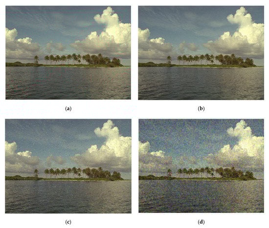
Figure 1.
Examples of the test image with different quality: (a) excellent (distortion type #2—additive noise in color components)—mean opinion score (MOS) = 6.15, peak signal-to-noise ratio (PSNR) = 40.773 dB, PSNRHA = 36.935 dB, Mean Deviation Similarity Index (MDSI) = 0.19; (b) good (distortion type #5—high frequency noise)—MOS = 5.6154, PSNR = 34.799 dB, PSNRHA = 39.5 dB, MDSI = 0.1892; (c) middle (distortion type #6—impulse noise)—MOS = 3.9737, PSNR = 27.887 dB, PSNRHA = 29.208 dB, MDSI = 0.3413; (d) bad (distortion type #3—spatially correlated noise)—MOS = 3.2368, PSNR = 28.842 dB, PSNRHA = 26.1 dB, MDSI = 0.3887.
Taking this into account, it has been decided that the NN output should be in the same limits as the MOS. This means that error minimization with respect to MOS can be used as the target function in the NN training. If needed, MOS (NN output) can be easily recalculated to another scale like, e.g., from 0 to 1.
The penultimate question concerns input pre-processing. It is known that it is often recommended in the NN theory to carry out some preliminary normalization of input data (features) if they have different ranges of variation [61]. This is true for elementary metrics, as for example, PSNR and PSNR-HVS-M, both expressed in dB, can vary in wide limits (even from 10 dB to 60 dB) but, for distorted images in TID2013, they vary in narrower limits. PSNR used for setting five levels of distortions, has five values approximately reached (21, 24, 27, 30, and 33 dB) although, in fact, the values of this metric for images in TID2013 vary from about 13 dB to ≈41 dB. Consecutively, PSNR-HVS-M varies from 14 dB to 59 dB, which mainly corresponds to “operation limits” starting from very annoying distortions to practically perfect quality (invisible distortions). The MDSI varies from 0.1 to 0.55 for images in TID2013 where the larger values correspond to lower visual quality. Some other metrics like SSIM, MS-SSIM, and FSIM vary in the limits from 0 to 1, where the latter limit corresponds to perfect quality. In fact, most values of these metrics are concentrated in the upper third part of this interval (see the scatter plot in Figure 2 for the color version of the metric FSIM, referred to as FSIMc). An obvious general tendency of the increase in FSIMc when MOS becomes larger is observed. Meanwhile, two important phenomena may also be noticed. Firstly, there is a certain diversity of the metric’s values for the same MOS. Secondly, the dependence of FSIMc on MOS (or MOS on FSIMc) is nonlinear.
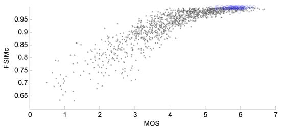
Figure 2.
The scatter plot of color version of Feature SIMilarity (FSIMc) vs. MOS (blue circles correspond to images for which distortions have not been detected).
In this sense, linearization (fitting) is often used to get not only the high values of SROCC but the conventional (Pearson) correlation factor (coefficient) as well [69]. Then, two hypotheses are possible. The first one is that the NN, being nonlinear and able to adapt to peculiarities of input data, will “manage” this nonlinearity of input–output dependence “by itself” (denote this hypothesis as H1). The second hypothesis (H2) is that elementary metric pre-processing in the form of fitting can be beneficial for further improvement of combined metric performance (optimization).
Concerning fitting needed for realization of H2, there are several commonly accepted options. One of them is to apply the Power Fitting Function (PFF) y(x) = a ∙ xb + c, where a, b, and c are the adjustable parameters. The fitting results can be characterized by the root mean square error (RMSE) of the scatter plot points after fitting with respect to the fitted curve (the smaller RMSE, the better). The results obtained for the elementary metrics considered above (in Table 2) are given in the left part of Table 3. As one can see, the best fitting result (the smallest RMSE) is obtained for the metric MDSI (it equals to 0.3945). The results for the metrics that are among the best according to SROCC, e.g., Contrast and Visual Saliency Similarity Induced index (CVSSI), Multiscale Contrast Similarity Deviation (MCSD), PSNRHA, Gradient Magnitude Similarity Deviation (GMSD), see data in Table 2, are almost equally good, too.
Table 3.
Metric fitting results and parameters for the Power Fitting Function (PFF) and second order polynomial (Poly2); better RMSE values are shown in bold format.
Another fitting model that can be applied is, e.g., Poly2 y(x) = p1 ∙ x2 + p2 ∙ x + p3, where p1, p2, and p3 are parameters to be adjusted to produce the best fit. The results are very similar. For example, for MDSI, the minimal RMSE equal to 0.3951 is observed. For PSNRHA, RMSE = 0.4013 is achieved, i.e., slightly better than using the PFF. The detailed data obtained for Poly2 fit are presented in the right part of Table 3. For clarity, the better of the two RMSE results are marked by the bold format in Table 3. Then, three options are possible in combined NN design: 1) to use the PFF for all elementary metrics; 2) to apply Poly2 for all elementary metrics; 3) to choose the best fitting for each elementary metric and to apply it.
Earlier in [53], different possible monotonous functions including linear fitting have been considered for combining elementary metrics. As practice has shown, they produce worse results with higher RMSE in comparison to PFF and Poly2.
The next considered issue is what structures and parameters of NNs can be chosen and optimized. As it has been noted above, we concentrate on conventional structures. We prefer to apply the multilayer NN instead of a deep learning approach because in this way many design aspects are clear. It prevents the overtraining problems and allows for a good generalization. In particular, the number of neurons in the input layer can be equal to the number of elementary metrics used. In addition, this solution can be easily adopted by using TID2013, avoiding the need for a large training set of data.
Concerning this number, different options are possible, including the use of all 50 considered elementary metrics. It is also possible to restrict to the best metrics from Table 2 and employ elementary metrics that have certain properties, for example, metrics that have SROCC > 0.9 for the considered types of distortions (there are 22 such metrics), SROCC > 0.92 (14 metrics), or SROCC > 0.93 (7 metrics).
Nevertheless, the theory of NNs states that it is reasonable to apply such input parameters that can “add” or “complement” information to each other, i.e., are not highly correlated. One possible approach is the evaluation of cross-correlation function to determine the similarity between all pairs of metrics and after that to exclude the worst in highly correlated pairs.
Instead of that, in this paper, a very useful approach called Lasso regularization [111] (Lasso is an abbreviation for Least Absolute Shrinkage and Selection Operator) has been applied for the selection of the most unique metrics for NNs. In machine learning, Lasso and Ridge regularizations are used to introduce additional limitations to the model and decrease the problem of overfitting.
The key feature of Lasso is that this method may introduce zero weights for the “noisy” and the least important data. For the task of metrics combination, it means that Lasso regularization can determine the elementary metrics that are the least useful for combining and leave the other (“most informative”) ones. This study adopts the implementation of Lasso available in MATLAB® so that, for different thresholds, zero coefficients for metrics that can be excluded can be estimated. According to that, the number of such non-zero values (NNZ) for each metric has been determined, assuming the following conditions: (a) NNZ > 20 (out of 100 values); (b) NNZ > 30; (c) NNZ > 40; (d) NNZ > 50; (e) NNZ > 60.
Since the network output is the combined metric, one neuron is present in the output layer, but the number of hidden layers and the number of neurons in each hidden layer can be different. Two variants have been analyzed—two and four hidden layers. Furthermore, two variants of the numbers of neurons in the hidden layers have been considered, namely an equal number of neurons in each hidden layer and a twice smaller number of neurons in each successive hidden layer.
As the activation function in hidden layers, the hyperbolic tangent sigmoid transfer function is used, which also provides the normalization in the range (−1,1), whereas a linear function is used for the output layer.
An example of the NN structure is presented in Figure 3. In this case, there are nine inputs and the number of neurons in hidden layers decreases gradually.
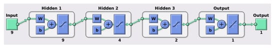
Figure 3.
An exemplary structure of the neural network with 9 inputs used in experiments.
In addition to the NN structure, some other factors might influence its performance, such as the methodology of NN training and testing, stability of training results, the number of epochs, etc. Due to the limited set of 1625 images for the NN training and testing, this constraint complicates our task. According to a traditional methodology, an available set should be divided into training and verification ones in some proportion. In the conducted experiments, 70% of images have been used for training and the remaining images for verification. Since the division of images into sets is random, training and verification results can be random as well. To partly get around this uncertainty, the best data are presented below for each version of the trained NN (producing the largest SROCC at training stage) of a given structure.
Concerning the training stage—each NN has been trained to provide as high SROCC as possible. Obviously, some other training strategies are also possible. In particular, it is possible to use the Pearson correlation coefficient (PCC) to be maximized. Nevertheless, the results of the additional use of the PCC for the training are not considered in this paper.
To give more understanding of which NN structures have been analyzed and what parameters have been used, the main characteristics are presented in Table 4, where the number of input elementary metrics is provided in each case. As can be seen, there are quite a lot of possible NN structures.
Table 4.
The numbers of elementary metrics used as the inputs for different configurations of neural networks (NN)s under conditions of different fitting and restrictions imposed on an elementary metric set.
6. Neural Network Training and Verification Results
The main criteria of the NN training and verification are the SROCC values. Four SROCCs have been analyzed: SROCCtrain(Max), SROCCtrain(Lasso), SROCCtest(Max), and SROCCtest(Lasso) that correspond to the training and test (verification) cases using maximal and Lasso-determined numbers of inputs. Starting from the NN with two hidden layers, where preliminary fitting is not used, the obtained results are presented in Figure 4. Digits near each point in the presented plots show the numbers of neurons in hidden layers. Data in Figure 4a relate to the case when the numbers of neurons in hidden layers are the same, whilst the plots in Figure 4b correspond to situation when the numbers of neurons steadily diminish.
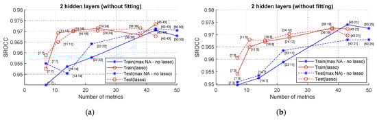
Figure 4.
SROCC values for NNs with two hidden layers with different numbers of inputs: (a) equal number of neurons in hidden layers; (b) twice smaller number of neurons in hidden layers.
The analysis of data shows the following:
- If Lasso is not used, the increase in the number of metrics leads to a general tendency of increasing both SROCCtrain and SROCCtest; meanwhile, for more than 40 inputs, the improvement is not observed;
- If Lasso regularization is applied, the results are not so good if the number of inputs (Ninp) is smaller than 20; but if it exceeds 20, the performance practically does not depend on Ninp; this means that the Lasso method allows the simplification of the NN structure, minimizing the number of inputs and neurons in the other layers;
- The best (largest) SROCC values exceed 0.97, demonstrating that a sufficient improvement (compared to the best elementary metric) is attained due to the use of the NN and parameters’ optimization;
- SROCCtrain and SROCCtest are practically the same for each configuration of the analyzed NN, so training results can be considered as stable;
- No essential difference in results has been found for equal or non-equal numbers of neurons in hidden layers.
Concerning another number of hidden layers, namely four, the obtained plots are given in Figure 5. The analysis of the obtained data makes it possible to draw two main conclusions. Firstly, there are no obvious advantages in comparison to the case of using NNs with two hidden layers. Secondly, for all other conclusions given above, concerning SROCCtrain and SROCCtest, the influence of Ninp and Lasso regularization are the same, i.e., it is reasonable to apply a limited number, e.g., 24 elementary metrics determined by Lasso.
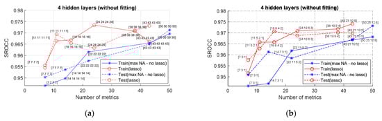
Figure 5.
SROCC values for NNs with four hidden layers with different numbers of inputs: (a) equal number of neurons in hidden layers; (b) twice smaller number of neurons in hidden layers.
The next question to be answered is: “does preliminary fitting help?” The answer to it is presented in Figure 6 with two sets of plots. Both sets are obtained for the NNs with two hidden layers and with an equal number of neurons in them. The plots in Figure 6a are obtained for the PFF, and in Figure 6b—for the best fit. A comparison of the plots corresponding to each other in Figure 6 shows that there is no sufficient difference in the choice of fitting. Moreover, comparison to the corresponding plots in Figure 4a indicates that preliminary fitting does not produce sufficient performance improvement compared to the cases when it is not used. This means that the trained NNs provide this pre-processing by themselves.
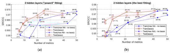
Figure 6.
SROCC values for NNs with two hidden layers with different numbers of inputs and an equal number of neurons in hidden layers with two ways of fitting: (a) PFF; (b) the best fitting.
The other conclusions that stem from the analysis of the plots in Figure 6 are practically the same as earlier. The lasso method ensures that the performance close to optimal can be provided for Ninp slightly larger than 20. The maximal attained values of SROCC are above 0.97 and smaller than 0.975. The results for four hidden layers and non-equal numbers of neurons in the hidden layers have been analyzed as well, and the best results are practically at the same level.
To prove that the number of hidden layers does not have any essential influence on the performance of the combined NN-based metrics, the metric characteristics for three and five hidden layers of NNs that used PFF for elementary metric pre-processing and equal numbers of neurons in all layers are presented in Figure 7. The analysis shows that the maximal attained values of the SROCC are even smaller than for NNs with two layers.
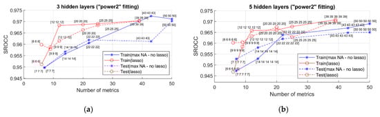
Figure 7.
SROCC values for NNs with equal numbers of neurons in hidden layers for PFF with: (a) three layers; (b) five layers.
Completing the analysis based on SROCC, it is possible to state the following:
- there are many configurations of NNs that provide approximately the same SROCC;
- keeping in mind the desired simplicity, the use of NNs with two hidden layers without fitting, and with a number of inputs of about 20, is recommended.
Nevertheless, two other aspects are interesting as well—what are the elementary metrics “recommended” by Lasso in this case, and are the conclusions drawn from SROCC analysis in agreement with conclusions that stem from the analysis for other criteria? Answering the first question, two good NN configurations can be found in Figure 4a, namely NNs with 16 and 24 inputs. The elementary metrics used by the NN with 16 inputs, as well as with 24 inputs, are listed in Table 5. As can be seen, all 16 metrics from the first set are also present in the second set.
Table 5.
Elementary metrics used by the neural network for 16 and 24 inputs with SROCC values.
The first observation is that the metrics MDSI, CVSSI, PSNRHA, GMSD, IGM, HaarPSI, ADM, IQM2, which are among the top-20 in Table 2, are present among the chosen ones. Some moderately good metrics, such as DSS, are also chosen. There are elementary metrics that are efficient according to data in Table 2 but they are not chosen, for example, MCSD, PSNRHMAm, PSIM. Although for PSNRHMAm, the reason for excluding this metric by Lasso may be its high correlation with PSNRHVS and PSNRHA, the situation is not as clear for MCSD and PSIM. Meanwhile, the sets contain such metrics as WASH and MSVD that, according to data in Table 2, do not perform well. In addition, both sets contain PSNR, and the second set also contains MSE, strictly connected to PSNR. This means that, although Lasso allows making the sets of recommended elementary metrics narrower, the result of its operation is not optimal.
Nevertheless, there are several positive outcomes of the design using Lasso. They become obvious from the analysis of data presented in Table 6. It may be observed that there are several good configurations of NNs that provide a SROCC of about 0.97 for the number of inputs of about 20 (this is also shown in plots). Moreover, these NNs ensure RMSE values that are considerably smaller than for the best elementary metric after linearization (see data in Table 3 where the best values are larger than 0.39). In addition, the values of the Pearson correlation coefficient (PCC) are also large and exceed 0.97, indicating very good linearity properties of the designed combined metrics.
Table 6.
Performance characteristics of designed NN-based combined quality metrics.
Having calculated the SROCC, RMSE and PCC values, it is possible to carry out a more thorough analysis. The first observation is that SROCC, RMSE and PCC are highly correlated in our case. Larger SROCC and PCC correspond to smaller RMSE. The best results, according to all three criteria, are produced by the NN with configuration #3, although, considering the NN complexity, the configuration #2 is good as well. The number of inputs smaller than 16 (e.g., 11 or 12 in configurations #1, #4, #5) leads to worse values of the considered criteria. The use of the NN configurations with preliminary fitting, a decreasing number of neurons in hidden layers, and a larger number of hidden layers (configurations ##4–9), does not produce improvements in comparison to the corresponding configurations #1 and #2. Thus, the application of the NN configuration #2 will be further analyzed.
Table 6 contains three columns marked by the heading “The best network” and three columns marked by “The top 5 results”. It has been mentioned earlier that the results of the NN learning depend on the random division of distorted images into training and testing sets. Because of this, to analyze the stability of training, we have calculated the mean SROCC, RMSE and PCC values for the top five results of NN training for each configuration as well as their standard deviations provided in brackets. A comparison of SROCC, RMSE and PCC for the top five results to the corresponding values for the best network shows that the difference is small. Moreover, the conclusions that can be drawn as the result of the analysis of these “average” results concerning NN performance fully coincide with conclusions drawn from the analysis for the best network.
7. Analysis of Computational Efficiency
In addition, the computational efficiency should be briefly discussed. For the NN-based metric with 16 inputs, the calculation of PSNR, MDSI, PSNRHVS, ADM, GMSD, WASH, IQM2, CVSSI and HaarPSI is very fast or fast, the calculation of IFC and RFSIM requires several times longer, whereas the calculation of MSVD, CWSSIM, PSNRHA, IGM, and DSI, takes even more time (about one order of magnitude). Thus, even with parallel calculations of elementary metrics, a calculation of the NN-based metric needs sufficiently more time than for such good elementary metrics as MDSI, GMSD or HaarPSI.
Hence, further research directions should be directed to the combination of possibly fast elementary metrics, providing a possibly good balance between the MOS prediction monotonicity (as well as accuracy) and computational efficiency. The average calculation time of the considered elementary metrics determined for 512 × 384 pixels images from the TID2013 dataset is provided in Table 7. Time data was evaluated using a notebook with Intel i5 4th generation CPU and 8 GB RAM controlled by the Linux Ubuntu 18.04 operating system, using MATLAB® 2019b software.
Table 7.
Average calculation time for the images from the TID2013 database.
8. Verification for Three-Channel Remote Sensing Images
The analysis of metrics’ performance and their verification for multichannel RS images is a complex problem. Obviously, the best solution could be to have a database of reference and distorted RS images and MOS for each distorted image. This way of a future research is, in general, possible and expedient but it requires considerable time and effort. Firstly, a large number of observers have to be attracted to experiments. Secondly, these observers should have some skills in the analysis of RS data; this is the main problem. Thirdly, the set of images to be viewed and assessed has to be somehow agreed in the RS community.
Because of this, we are currently able to perform only some preliminary tests. The aim of the very first test is to show that the designed metric (in fact, MOS predicted by the trained NN) produces reasonable results for particular images. Regarding the images of Figure 1, for each of them the true MOS value is available. Furthermore, processing the value of each metric (PSNR, PSNRHA, MDSI) by using the linearization with the parameters previously processed (power fitting function) is also possible to obtain the corresponding estimation of MOS. Comparing these values with the MOS value predicted by NN (Table 8), it is clear that NN provides good results. Generalizing from this specific case to the TID2013 Noise&Actual subset, an interesting scatter plot can be obtained (Figure 8). A remarkable aspect is that the MOS values predicted from the selected elementary metrics can even be negative, whereas this drawback is absent when the MOS values are predicted by using NN. It is also seen that the NN-based metric provides high linearity of the relation between true and predicted MOS. Problems of MDSI for small MOS values are observed as well.
Table 8.
True and Predicted MOS Values.
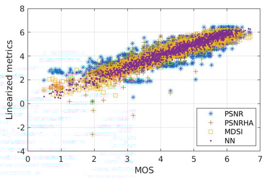
Figure 8.
Scatter plot illustrating the correlation of the four methods of MOS prediction presented in Table 8 with true MOS values (range 0–7) for the TID2013 Noise&Actual subset.
The further studies relate to four test images presented in Figure 9. These are three-channel pseudo-color images called Frisco, Diego2, Diego3, and Diego4, respectively, all of size 512 × 512 pixels, 24 bits per pixel, from the visible range of the Landsat sensor. The reasons for choosing them are twofold, as these images are of different complexity and they have been already used in some experiments [112]. The images Frisco and Diego4 are quite simple since they contain large homogeneous regions, whereas the image Diego2 has a very complex structure (a lot of small-size details and textures), and the image Diego3 is of a medium complexity.

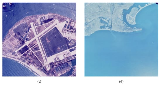
Figure 9.
Three-channel remote sensing (RS) test images: (a) Frisco; (b) Diego2; (c) Diego3; (d) Diego4.
A standard requirement of visual quality metrics is monotonicity, i.e., monotonous increasing or decreasing if the “intensity” of a given type of distortion increases. This property can be easily checked for many different types of distortions. These images have been compressed using the lossy AGU method [113], providing different quality and compression ratios (CR). This has been performed by changing the quantization step (QS) where a larger QS relates to larger introduced distortions and worse visual quality, respectively. Nevertheless, considering the possible extension of the proposed approach for multispectral RS images, as well as the highly demanded development of the RS image quality assessment database in the future, some more typical approaches to RS data compression should eventually be applied for this purpose, such as the CCSDS 123.0-B-2 standard [114].
The quality (excellent, good and so on) is determined according to the results in [61]. The collected data are presented in Table 9. An obvious tendency is that all metrics including the designed one become worse if QS (and CR, respectively) increases. The values of the NN-based metric are larger than MOS values predicted from elementary metrics for the test image Frisco, but smaller for the test image Diego2. Probably, this property is partly connected with image complexity. However, there are evidences that the designed metric “behaves” correctly. In Figure 10, the compressed images using QS = 40 are presented, for which distortions are always visible. A visual inspection (comparison) of these images to the reference images in Figure 9a,b shows that distortions are more visible for the test image Diego2. This is clearly confirmed by the values of PSNRHA (36.32 dB and 32.63 dB, respectively—see Table 9). PSNR shows the same tendency, although MDSI does not indicate this. Hence, some cases may be encountered when conclusions drawn from the analysis of different quality metrics can be different.
Table 9.
Predicted MOS Values for Two RS Test Images Using Linearization.
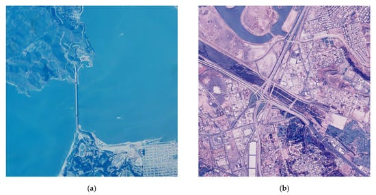
Figure 10.
Compressed images with quantization step (QS) = 40: (a) Frisco; (b) Diego2.
The analysis for the case of additive white Gaussian noise that has been added to the considered four three-channel images has also been carried out. Four values of noise variance have been used to correspond to four upper levels of distortions exploited in TID2013. The mean MOS values (averaged for 25 test images in TID2013) have also been obtained that correspond to these values of noise variance. For each image, PSNR, PSNRHA, and MDSI have been calculated and the corresponding predicted values of MOS have been determined. The NN-based metric has been calculated as well. The obtained results are presented in Table 10.
Table 10.
Predicted MOS values for four RS test images distorted by an additive white Gaussian noise.
The analysis shows that all metrics become worse (PSNR, PSNRHA and the designed metric decrease, and MDSI increases) if noise variance increases, i.e., the monotonicity property is preserved. The predicted MOS values are quite close to the mean MOS, whereas for good and middle quality PSNRHA, MDSI and the NN-based metric provide better MOS prediction than PSNR. However, for bad quality images, the situation is the opposite.
9. Conclusions
The task of assessing the visual quality of remote sensing images subject to different types of degradations has been considered. It has been shown that there are no commonly accepted metrics and, therefore, their design is desired. The problems that can be encountered have been mentioned and their solution has been proposed. The already existing database of distorted color images, for which it is possible to choose images with the types of distortions often observed in remote sensing, has been employed for this purpose. Its use allows the determination of existing visual quality metrics that perform well for the types of degradations that are of interest. The best of such metrics provides a SROCC with a MOS of about 0.93, which is considered as a very good result. Moreover, the database TID2013 allows the design of visual quality metrics based on the use of elementary visual quality metrics as inputs. Several configurations of NNs and methods of input data pre-processing have been studied. It has been shown that even simple NNs without input pre-processing (linearization) having two hidden layers are able to provide SROCC values of about 0.97. PCC values are of the same order, meaning that the relation between NN output and MOS values is practically linear.
Some elementary metrics and the designed one have then been verified for three-channel remote sensing images with two types of degradations, demonstrating the monotonicity of the proposed metric’s behavior. Besides, it has been shown that the designed metric produces an accurate evaluation of MOS that allows the classification of remote sensing images according to their quality. Since, as shown in the paper, from the visual quality point of view, color images and RS images (after applying the necessary operation to visualize them) have similar characteristics, this manuscript provides the first evidence that a full-reference image quality metric, developed using a dataset (TID2013) that is actually not a remote sensing dataset, works well when applied to RGB images obtained by remote sensing data.
In the future, the ways of accelerating NN-based metrics by means of restricting the set of possible inputs are planned to be analyzed, considering the computational efficiency of the input metrics as well. We also hope that some perceptual experiments, with the help of some specialists in RS image analysis for image quality assessment, will be carried out. Although for different types of RS data, different types of degradations can be important, we have considered only those ones that are quite general and are present in TID2013. For example, the characteristics of clouds can be additional feature(s) used as elementary metrics in the quality characterization of particular types of RS data in future research.
One of the limitations of the proposed method is the necessity of calculation of several metrics, which are not always fast. To overcome this issue, some of them may be calculated in parallel, although hardware acceleration possibilities should be provided in such cases.
Another shortcoming is the fact that many metrics are developed for grayscale images and hence they may be applied for single channel only (or independently for three channels leading to three independent results). Hence, a relevant direction of our further research will be related to the optimization of color to greyscale conversion methods used for the individual elementary metrics. In some cases, an appropriate application of elementary metrics for multichannel images may also require changes of data types and dynamic ranges. Although the color to greyscale conversion based on the International Telecommunication Union (ITU) Recommendation BT.601-5 (with the use of RGB to YCbCr conversion in fact limiting the range of the Y component to the range [16,235]), has been assumed in this paper, the results of individual elementary metrics obtained using various color spaces and conversion methods may lead to further increases in the combined metrics’ performance.
Author Contributions
Conceptualization, V.L.; Data curation, O.I. and K.O.; Formal analysis, V.L. and O.I.; Investigation, O.I. and K.O.; Methodology, V.L. and K.O.; Software, O.I.; Supervision, K.E.; Writing—original draft, V.L.; Writing—review & editing, K.E. All authors have read and agreed to the published version of the manuscript.
Funding
The research is partially co-financed by the Polish National Agency for Academic Exchange (NAWA) and the Ministry of Education and Science of Ukraine under the project no. PPN/BUA/2019/1/00074 entitled “Methods of intelligent image and video processing based on visual quality metrics for emerging applications”.
Acknowledgments
The Authors would like to thank the anonymous Reviewers as well as the Editor for their valuable comments and suggestions helping to improve the revised version of the paper.
Conflicts of Interest
The authors declare no conflict of interest. The funders had no role in the design of the study; in the collection, analyses, or interpretation of data; in the writing of the manuscript, or in the decision to publish the results.
References
- Schowengerdt, R.A. Remote Sensing, Models, and Methods for Image Processing, 3rd ed.; Academic Press: Burlington, MA, USA, 2007; ISBN 978-0-12-369407-2. [Google Scholar]
- Khorram, S.; van der Wiele, C.F.; Koch, F.H.; Nelson, S.A.C.; Potts, M.D. Future Trends in Remote Sensing. In Principles of Applied Remote Sensing; Springer International Publishing: Cham, Switzerland, 2016; pp. 277–285. ISBN 978-3-319-22559-3. [Google Scholar]
- Gonzalez-Roglich, M.; Zvoleff, A.; Noon, M.; Liniger, H.; Fleiner, R.; Harari, N.; Garcia, C. Synergizing global tools to monitor progress towards land degradation neutrality: Trends.Earth and the World Overview of Conservation Approaches and Technologies sustainable land management database. Environ. Sci. Policy 2019, 93, 34–42. [Google Scholar] [CrossRef]
- Marcuccio, S.; Ullo, S.; Carminati, M.; Kanoun, O. Smaller Satellites, Larger Constellations: Trends and Design Issues for Earth Observation Systems. IEEE Aerosp. Electron. Syst. Mag. 2019, 34, 50–59. [Google Scholar] [CrossRef]
- Kussul, N.; Lemoine, G.; Gallego, F.J.; Skakun, S.V.; Lavreniuk, M.; Shelestov, A. Parcel-Based Crop Classification in Ukraine Using Landsat-8 Data and Sentinel-1A Data. IEEE J. Sel. Top. Appl. Earth Obs. Remote Sens. 2016, 9, 2500–2508. [Google Scholar] [CrossRef]
- European Space Agency First Applications from Sentinel-2A. Available online: http://www.esa.int/Our_Activities/Observing_the_Earth/Copernicus/Sentinel-2/First_applications_from_Sentinel-2A (accessed on 8 May 2020).
- Joshi, N.; Baumann, M.; Ehammer, A.; Fensholt, R.; Grogan, K.; Hostert, P.; Jepsen, M.; Kuemmerle, T.; Meyfroidt, P.; Mitchard, E.; et al. A Review of the Application of Optical and Radar Remote Sensing Data Fusion to Land Use Mapping and Monitoring. Remote Sens. 2016, 8, 70. [Google Scholar] [CrossRef]
- Deledalle, C.-A.; Denis, L.; Tabti, S.; Tupin, F. MuLoG, or How to Apply Gaussian Denoisers to Multi-Channel SAR Speckle Reduction? IEEE Trans. Image Process. 2017, 26, 4389–4403. [Google Scholar] [CrossRef] [PubMed]
- Zhong, P.; Wang, R. Multiple-Spectral-Band CRFs for Denoising Junk Bands of Hyperspectral Imagery. IEEE Trans. Geosci. Remote Sens. 2013, 51, 2260–2275. [Google Scholar] [CrossRef]
- Ponomaryov, V.; Rosales, A.; Gallegos, F.; Loboda, I. Adaptive Vector Directional Filters to Process Multichannel Images. IEICE Trans. Commun. 2007, E90-B, 429–430. [Google Scholar] [CrossRef]
- Van Zyl Marais, I.; Steyn, W.H.; du Preez, J.A. Onboard image quality assessment for a small low earth orbit satellite. In Proceedings of the 7th IAA Symposium on Small Satellites for Earth Observation, Berlin, Germany, 4–8 May 2009. Paper IAA B7-0602. [Google Scholar]
- Hagolle, O.; Huc, M.; Pascual, D.V.; Dedieu, G. A multi-temporal method for cloud detection, applied to FORMOSAT-2, VENµS, LANDSAT and SENTINEL-2 images. Remote Sens. Environ. 2010, 114, 1747–1755. [Google Scholar] [CrossRef]
- Li, X.; Wang, L.; Cheng, Q.; Wu, P.; Gan, W.; Fang, L. Cloud removal in remote sensing images using nonnegative matrix factorization and error correction. ISPRS J. Photogramm. Remote Sens. 2019, 148, 103–113. [Google Scholar] [CrossRef]
- Li, Y.; Clarke, K.C. Image deblurring for satellite imagery using small-support-regularized deconvolution. ISPRS J. Photogramm. Remote Sens. 2013, 85, 148–155. [Google Scholar] [CrossRef]
- Xia, H.; Liu, C. Remote Sensing Image Deblurring Algorithm Based on WGAN. In Service-Oriented Computing—ICSOC 2018 Workshops; Liu, X., Mrissa, M., Zhang, L., Benslimane, D., Ghose, A., Wang, Z., Bucchiarone, A., Zhang, W., Zou, Y., Yu, Q., Eds.; Lecture Notes in Computer Science; Springer International Publishing: Cham, Switzerland, 2019; Volume 11434, pp. 113–125. ISBN 978-3-030-17641-9. [Google Scholar]
- Christophe, E. Hyperspectral Data Compression Tradeoff. In Optical Remote Sensing; Prasad, S., Bruce, L.M., Chanussot, J., Eds.; Springer: Berlin/Heidelberg, Germany, 2011; pp. 9–29. ISBN 978-3-642-14211-6. [Google Scholar]
- Blanes, I.; Magli, E.; Serra-Sagrista, J. A Tutorial on Image Compression for Optical Space Imaging Systems. IEEE Geosci. Remote Sens. Mag. 2014, 2, 8–26. [Google Scholar] [CrossRef]
- Zemliachenko, A.N.; Kozhemiakin, R.A.; Uss, M.L.; Abramov, S.K.; Ponomarenko, N.N.; Lukin, V.V.; Vozel, B.; Chehdi, K. Lossy compression of hyperspectral images based on noise parameters estimation and variance stabilizing transform. J. Appl. Remote Sens. 2014, 8, 083571. [Google Scholar] [CrossRef]
- Penna, B.; Tillo, T.; Magli, E.; Olmo, G. Transform Coding Techniques for Lossy Hyperspectral Data Compression. IEEE Trans. Geosci. Remote Sens. 2007, 45, 1408–1421. [Google Scholar] [CrossRef]
- Xu, T.; Fang, Y. Remote sensing image interpolation via the nonsubsampled contourlet transform. In Proceedings of the 2010 International Conference on Image Analysis and Signal Processing, Zhejiang, China, 9–11 April 2010; pp. 695–698. [Google Scholar]
- Al-Shaykh, O.K.; Mersereau, R.M. Lossy compression of noisy images. IEEE Trans. Image Process. 1998, 7, 1641–1652. [Google Scholar] [CrossRef] [PubMed]
- Shi, X.; Wang, L.; Shao, X.; Wang, H.; Tao, Z. Accurate estimation of motion blur parameters in noisy remote sensing image. In Proceedings of the SPIE Sensing Technology + Applications; Huang, B., Chang, C.-I., Lee, C., Li, Y., Du, Q., Eds.; SPIE: Baltimore, MD, USA, 21 May 2015; p. 95010X. [Google Scholar]
- Abramov, S.; Uss, M.; Lukin, V.; Vozel, B.; Chehdi, K.; Egiazarian, K. Enhancement of Component Images of Multispectral Data by Denoising with Reference. Remote Sens. 2019, 11, 611. [Google Scholar] [CrossRef]
- Dellepiane, S.G.; Angiati, E. Quality Assessment of Despeckled SAR Images. IEEE J. Sel. Top. Appl. Earth Obs. Remote Sens. 2014, 7, 691–707. [Google Scholar] [CrossRef]
- Rubel, O.; Lukin, V.; Rubel, A.; Egiazarian, K. NN-Based Prediction of Sentinel-1 SAR Image Filtering Efficiency. Geosciences 2019, 9, 290. [Google Scholar] [CrossRef]
- Rubel, O.; Rubel, A.; Lukin, V.; Carli, M.; Egiazarian, K. Blind Prediction of Original Image Quality for Sentinel SAR Data. In Proceedings of the 2019 8th European Workshop on Visual Information Processing (EUVIP), Rome, Italy, 28–31 October 2019; pp. 105–110. [Google Scholar]
- Christophe, E.; Leger, D.; Mailhes, C. Quality criteria benchmark for hyperspectral imagery. IEEE Trans. Geosci. Remote Sens. 2005, 43, 2103–2114. [Google Scholar] [CrossRef]
- García-Sobrino, J.; Blanes, I.; Laparra, V.; Camps-Valls, G.; Serra-Sagristà, J. Impact of Near-Lossless Compression of IASI L1C data on Statistical Retrieval of Atmospheric Profiles. In Proceedings of the 4th On-Board Payload Data Compression Workshop (OBPDC), Venice, Italy, 23–24 October 2014. [Google Scholar]
- Lukin, V.; Abramov, S.; Krivenko, S.; Kurekin, A.; Pogrebnyak, O. Analysis of classification accuracy for pre-filtered multichannel remote sensing data. Expert Syst. Appl. 2013, 40, 6400–6411. [Google Scholar] [CrossRef]
- Hanley, J.A.; McNeil, B.J. A method of comparing the areas under receiver operating characteristic curves derived from the same cases. Radiology 1983, 148, 839–843. [Google Scholar] [CrossRef]
- Congalton, R.G.; Green, K. Assessing the Accuracy of Remotely Sensed Data: Principles and Practices; Mapping science series; Lewis Publications: Boca Raton, FL, USA, 1999; ISBN 978-0-87371-986-5. [Google Scholar]
- Zhou, H.; Gao, H.; Tian, X. A Super-resolution Reconstruction Method of Remotely Sensed Image Based on Sparse Representation. Sens. Transducers J. 2013, 160, 229–236. [Google Scholar]
- Aswathy, C.; Sowmya, V.; Soman, K.P. Hyperspectral Image Denoising Using Low Pass Sparse Banded Filter Matrix for Improved Sparsity Based Classification. Procedia Comput. Sci. 2015, 58, 26–33. [Google Scholar] [CrossRef][Green Version]
- Kumar, T.G.; Murugan, D.; Rajalakshmi, K.; Manish, T.I. Image enhancement and performance evaluation using various filters for IRS-P6 Satellite Liss IV remotely sensed data. Geofizika 2015, 32, 179–189. [Google Scholar] [CrossRef]
- Yang, K.; Jiang, H. Optimized-SSIM Based Quantization in Optical Remote Sensing Image Compression. In Proceedings of the 2011 Sixth International Conference on Image and Graphics, Hefei, China, 12–15 August 2011; pp. 117–122. [Google Scholar]
- Khosravi, M.R.; Sharif-Yazd, M.; Moghimi, M.K.; Keshavarz, A.; Rostami, H.; Mansouri, S. MRF-Based Multispectral Image Fusion Using an Adaptive Approach Based on Edge-Guided Interpolation. J. Geogr. Inf. Syst. 2017, 9, 114–125. [Google Scholar] [CrossRef]
- Agudelo-Medina, O.A.; Benitez-Restrepo, H.D.; Vivone, G.; Bovik, A. Perceptual Quality Assessment of Pan-Sharpened Images. Remote Sens. 2019, 11, 877. [Google Scholar] [CrossRef]
- Moreno-Villamarin, D.E.; Benitez-Restrepo, H.D.; Bovik, A.C. Predicting the Quality of Fused Long Wave Infrared and Visible Light Images. IEEE Trans. Image Process. 2017, 26, 3479–3491. [Google Scholar] [CrossRef] [PubMed]
- Jagalingam, P.; Hegde, A.V. A Review of Quality Metrics for Fused Image. Aquat. Procedia 2015, 4, 133–142. [Google Scholar] [CrossRef]
- Yuan, T.; Zheng, X.; Hu, X.; Zhou, W.; Wang, W. A Method for the Evaluation of Image Quality According to the Recognition Effectiveness of Objects in the Optical Remote Sensing Image Using Machine Learning Algorithm. PLoS ONE 2014, 9, e86528. [Google Scholar] [CrossRef]
- Wang, Z.; Bovik, A.; Sheikh, H.; Simoncelli, E. Image quality assessment: From error visibility to Structural Similarity. IEEE Trans. Image Process. 2004, 13, 600–612. [Google Scholar] [CrossRef]
- Wang, Z.; Bovik, A. A universal image quality index. IEEE Signal Process. Lett. 2002, 9, 81–84. [Google Scholar] [CrossRef]
- Guo, J.; Yang, F.; Tan, H.; Wang, J.; Liu, Z. Image matching using structural similarity and geometric constraint approaches on remote sensing images. J. Appl. Remote Sens. 2016, 10, 045007. [Google Scholar] [CrossRef]
- Liu, D.; Li, Y.; Chen, S. No-reference remote sensing image quality assessment based on the region of interest and structural similarity. In Proceedings of the 2nd International Conference on Advances in Image Processing—ICAIP ’18, Chengdu, China, 16–18 June 2018; ACM Press: New York, NY, USA, 2018; pp. 64–67. [Google Scholar]
- Krivenko, S.S.; Abramov, S.K.; Lukin, V.V.; Vozel, B.; Chehdi, K. Lossy DCT-based compression of remote sensing images with providing a desired visual quality. In Proceedings of the Image and Signal Processing for Remote Sensing XXV; Bruzzone, L., Bovolo, F., Benediktsson, J.A., Eds.; SPIE: Strasbourg, France, 7 October 2019; p. 36. [Google Scholar]
- Lin, W.; Jay Kuo, C.-C. Perceptual visual quality metrics: A survey. J. Vis. Commun. Image Represent. 2011, 22, 297–312. [Google Scholar] [CrossRef]
- Chandler, D.M. Seven Challenges in Image Quality Assessment: Past, Present, and Future Research. ISRN Signal Process. 2013, 2013, 1–53. [Google Scholar] [CrossRef]
- Niu, Y.; Zhong, Y.; Guo, W.; Shi, Y.; Chen, P. 2D and 3D Image Quality Assessment: A Survey of Metrics and Challenges. IEEE Access 2019, 7, 782–801. [Google Scholar] [CrossRef]
- Zhai, G.; Min, X. Perceptual image quality assessment: A survey. Sci. China Inf. Sci. 2020, 63, 211301. [Google Scholar] [CrossRef]
- Ponomarenko, N.; Jin, L.; Ieremeiev, O.; Lukin, V.; Egiazarian, K.; Astola, J.; Vozel, B.; Chehdi, K.; Carli, M.; Battisti, F.; et al. Image database TID2013: Peculiarities, results and perspectives. Signal Process. Image Commun. 2015, 30, 57–77. [Google Scholar] [CrossRef]
- Lin, H.; Hosu, V.; Saupe, D. KADID-10k: A Large-scale Artificially Distorted IQA Database. In Proceedings of the 2019 Eleventh International Conference on Quality of Multimedia Experience (QoMEX), Berlin, Germany, 5–7 June 2019; pp. 1–3. [Google Scholar]
- Sun, W.; Zhou, F.; Liao, Q. MDID: A multiply distorted image database for image quality assessment. Pattern Recognit. 2017, 61, 153–168. [Google Scholar] [CrossRef]
- Ieremeiev, O.; Lukin, V.; Ponomarenko, N.; Egiazarian, K. Robust linearized combined metrics of image visual quality. Electron. Imaging 2018, 2018, 260-1–260-6. [Google Scholar] [CrossRef]
- Okarma, K. Combined Full-Reference Image Quality Metric Linearly Correlated with Subjective Assessment. In Artificial Intelligence and Soft Computing; Rutkowski, L., Scherer, R., Tadeusiewicz, R., Zadeh, L.A., Zurada, J.M., Eds.; Lecture Notes in Computer Science; Springer: Berlin/Heidelberg, Germany, 2010; Volume 6113, pp. 539–546. ISBN 978-3-642-13207-0. [Google Scholar]
- Okarma, K. Combined image similarity index. Opt. Rev. 2012, 19, 349–354. [Google Scholar] [CrossRef]
- Okarma, K. Extended Hybrid Image Similarity—Combined Full-Reference Image Quality Metric Linearly Correlated with Subjective Scores. Electron. Electr. Eng. 2013, 19, 129–132. [Google Scholar] [CrossRef]
- Liu, T.-J.; Lin, W.; Kuo, C.-C.J. Image Quality Assessment Using Multi-Method Fusion. IEEE Trans. Image Process. 2013, 22, 1793–1807. [Google Scholar] [CrossRef] [PubMed]
- Lukin, V.V.; Ponomarenko, N.N.; Ieremeiev, O.I.; Egiazarian, K.O.; Astola, J. Combining Full-Reference Image Visual Quality Metrics by Neural Network; Rogowitz, B.E., Pappas, T.N., de Ridder, H., Eds.; International Society for Optics and Photonics: San Francisco, CA, USA, 2015; p. 93940K. [Google Scholar]
- Bosse, S.; Maniry, D.; Muller, K.-R.; Wiegand, T.; Samek, W. Deep Neural Networks for No-Reference and Full-Reference Image Quality Assessment. IEEE Trans. Image Process. 2018, 27, 206–219. [Google Scholar] [CrossRef]
- Bosse, S.; Maniry, D.; Wiegand, T.; Samek, W. A deep neural network for image quality assessment. In Proceedings of the 2016 IEEE International Conference on Image Processing (ICIP), Phoenix, AZ, USA, 25–28 September 2016; pp. 3773–3777. [Google Scholar]
- Ponomarenko, N.; Lukin, V.; Astola, J.; Egiazarian, K. Analysis of HVS-Metrics’ Properties Using Color Image Database TID. In Advanced Concepts for Intelligent Vision Systems; Battiato, S., Blanc-Talon, J., Gallo, G., Philips, W., Popescu, D., Scheunders, P., Eds.; Lecture Notes in Computer Science; Springer International Publishing: Cham, Switzerland, 2015; Volume 9386, pp. 613–624. ISBN 978-3-319-25902-4. [Google Scholar]
- Lukin, V.; Zemliachenko, A.; Krivenko, S.; Vozel, B.; Chehdi, K. Lossy Compression of Remote Sensing Images with Controllable Distortions. In Satellite Information Classification and Interpretation; B. Rustamov, R., Ed.; IntechOpen: London, UK, 2019; ISBN 978-1-83880-566-1. [Google Scholar]
- Yule, G.U.; Kendall, M.G. An Introduction to the Theory of Statistics, 14th ed.; Charles Griffin & Co.: London, UK, 1950. [Google Scholar]
- Goossens, B.; Pizurica, A.; Philips, W. Removal of Correlated Noise by Modeling the Signal of Interest in the Wavelet Domain. IEEE Trans. Image Process. 2009, 18, 1153–1165. [Google Scholar] [CrossRef] [PubMed]
- Ponomarenko, N.; Silvestri, F.; Egiazarian, K.; Carli, M.; Astola, J.; Lukin, V. On between-coefficient contrast masking of DCT basis functions. In Proceedings of the Third International Workshop on Video Processing and Quality Metrics for Consumer Electronics, VPQM 2007, Scottsdale, AZ, USA, 25–26 January 2007; Volume 4. [Google Scholar]
- Wang, Z.; Simoncelli, E.P.; Bovik, A.C. Multiscale structural similarity for image quality assessment. In Proceedings of the 37th Asilomar Conference on Signals, Systems and Computers, Pacific Grove, CA, USA, 9–12 November 2003; pp. 1398–1402. [Google Scholar]
- Solomon, J.A.; Watson, A.B.; Ahumada, A. Visibility of DCT basis functions: Effects of contrast masking. In Proceedings of the IEEE Data Compression Conference (DCC’94), Snowbird, UT, USA, 29–31 March 1994; IEEE Computer Society Press: Los Alamitos, CA, USA, 1994; pp. 361–370. [Google Scholar]
- Avcibaş, I.; Sankur, B.; Sayood, K. Statistical evaluation of image quality measures. J. Electron. Imaging 2002, 11, 206–223. [Google Scholar] [CrossRef]
- Ziaei Nafchi, H.; Shahkolaei, A.; Hedjam, R.; Cheriet, M. Mean Deviation Similarity Index: Efficient and Reliable Full-Reference Image Quality Evaluator. IEEE Access 2016, 4, 5579–5590. [Google Scholar] [CrossRef]
- Gu, K.; Li, L.; Lu, H.; Min, X.; Lin, W. A Fast Reliable Image Quality Predictor by Fusing Micro- and Macro-Structures. IEEE Trans. Ind. Electron. 2017, 64, 3903–3912. [Google Scholar] [CrossRef]
- Zhang, L.; Shen, Y.; Li, H. VSI: A Visual Saliency-Induced Index for Perceptual Image Quality Assessment. IEEE Trans. Image Process. 2014, 23, 4270–4281. [Google Scholar] [CrossRef]
- Ponomarenko, N.; Ieremeiev, O.; Lukin, V.; Egiazarian, K.; Carli, M. Modified image visual quality metrics for contrast change and mean shift accounting. In Proceedings of the 2011 11th International Conference The Experience of Designing and Application of CAD Systems in Microelectronics (CADSM), Polyana-Svalyava, Ukraine, 23–35 February 2011; pp. 305–311. [Google Scholar]
- Ieremeiev, O.; Lukin, V.; Ponomarenko, N.; Egiazarian, K. Full-reference metrics multidistortional analysis. Electron. Imaging 2017, 2017, 27–35. [Google Scholar] [CrossRef]
- Sheikh, H.R.; Bovik, A.C. Image information and visual quality. IEEE Trans. Image Process. 2006, 15, 430–444. [Google Scholar] [CrossRef]
- Mansouri, A.; Aznaveh, A.M.; Torkamani-Azar, F.; Jahanshahi, J.A. Image quality assessment using the singular value decomposition theorem. Opt. Rev. 2009, 16, 49–53. [Google Scholar] [CrossRef]
- Ponomarenko, N.; Lukin, V.; Zelensky, A.; Egiazarian, K.; Carli, M.; Battisti, F. TID2008-a database for evaluation of full-reference visual quality assessment metrics. Adv. Mod. Radioelectron. 2009, 10, 30–45. [Google Scholar]
- Shnayderman, A.; Gusev, A.; Eskicioglu, A.M. An SVD-based grayscale image quality measure for local and global assessment. IEEE Trans. Image Process. 2006, 15, 422–429. [Google Scholar] [CrossRef] [PubMed]
- Zhang, L.; Zhang, L.; Mou, X.; Zhang, D. FSIM: A Feature Similarity Index for Image Quality Assessment. IEEE Trans. Image Process. 2011, 20, 2378–2386. [Google Scholar] [CrossRef] [PubMed]
- Zhang, L.; Zhang, L.; Mou, X. RFSIM: A feature based image quality assessment metric using Riesz transforms. In Proceedings of the 2010 IEEE International Conference on Image Processing, Hong Kong, China, 26–29 September 2010; pp. 321–324. [Google Scholar]
- Mitsa, T.; Varkur, K.L. Evaluation of contrast sensitivity functions for the formulation of quality measures incorporated in halftoning algorithms. In Proceedings of the IEEE International Conference on Acoustics Speech and Signal Processing, Minneapolis, MN, USA, 27–30 April 1993; Volume 5, pp. 301–304. [Google Scholar]
- Damera-Venkata, N.; Kite, T.D.; Geisler, W.S.; Evans, B.L.; Bovik, A.C. Image quality assessment based on a degradation model. IEEE Trans. Image Process. 2000, 9, 636–650. [Google Scholar] [CrossRef] [PubMed]
- Sheikh, H.R.; Bovik, A.C.; de Veciana, G. An information fidelity criterion for image quality assessment using natural scene statistics. IEEE Trans. Image Process. 2005, 14, 2117–2128. [Google Scholar] [CrossRef] [PubMed]
- Aja-Fernandez, S.; Estepar, R.S.J.; Alberola-Lopez, C.; Westin, C.-F. Image Quality Assessment based on Local Variance. In Proceedings of the 2006 International Conference of the IEEE Engineering in Medicine and Biology Society, New York, NY, USA, 30 August–3 September 2006; pp. 4815–4818. [Google Scholar]
- Egiazarian, K.; Astola, J.; Ponomarenko, N.; Lukin, V.; Battisti, F.; Carli, M. Two new full-reference quality metrics based on HVS. In Proceedings of the Second International Workshop on Video Processing and Quality Metrics, Scottsdale, AZ, USA, 22–24 January 2006; Volume 4. [Google Scholar]
- Chandler, D.M.; Hemami, S.S. VSNR: A Wavelet-Based Visual Signal-to-Noise Ratio for Natural Images. IEEE Trans. Image Process. 2007, 16, 2284–2298. [Google Scholar] [CrossRef]
- Sampat, M.P.; Wang, Z.; Gupta, S.; Bovik, A.C.; Markey, M.K. Complex Wavelet Structural Similarity: A New Image Similarity Index. IEEE Trans. Image Process. 2009, 18, 2385–2401. [Google Scholar] [CrossRef]
- Wang, Z.; Li, Q. Information Content Weighting for Perceptual Image Quality Assessment. IEEE Trans. Image Process. 2011, 20, 1185–1198. [Google Scholar] [CrossRef]
- Li, S.; Zhang, F.; Ma, L.; Ngan, K.N. Image Quality Assessment by Separately Evaluating Detail Losses and Additive Impairments. IEEE Trans. Multimed. 2011, 13, 935–949. [Google Scholar] [CrossRef]
- Liu, A.; Lin, W.; Narwaria, M. Image Quality Assessment Based on Gradient Similarity. IEEE Trans. Image Process. 2012, 21, 1500–1512. [Google Scholar] [CrossRef]
- Zhang, L.; Li, H. SR-SIM: A fast and high performance IQA index based on spectral residual. In Proceedings of the 2012 19th IEEE International Conference on Image Processing, Orlando, FL, USA, 30 September–3 October 2012; pp. 1473–1476. [Google Scholar]
- Zhang, X.; Feng, X.; Wang, W.; Xue, W. Edge Strength Similarity for Image Quality Assessment. IEEE Signal Process. Lett. 2013, 20, 319–322. [Google Scholar] [CrossRef]
- Chang, H.-W.; Yang, H.; Gan, Y.; Wang, M.-H. Sparse Feature Fidelity for Perceptual Image Quality Assessment. IEEE Trans. Image Process. 2013, 22, 4007–4018. [Google Scholar] [CrossRef] [PubMed]
- Reenu, M.; David, D.; Raj, S.S.A.; Nair, M.S. Wavelet Based Sharp Features (WASH): An Image Quality Assessment Metric Based on HVS. In Proceedings of the 2013 2nd International Conference on Advanced Computing, Networking and Security, Mangalore, India, 15–17 December 2013; pp. 79–83. [Google Scholar]
- Wu, J.; Lin, W.; Shi, G.; Liu, A. Perceptual Quality Metric with Internal Generative Mechanism. IEEE Trans. Image Process. 2013, 22, 43–54. [Google Scholar] [CrossRef] [PubMed]
- Xue, W.; Zhang, L.; Mou, X.; Bovik, A.C. Gradient Magnitude Similarity Deviation: A Highly Efficient Perceptual Image Quality Index. IEEE Trans. Image Process. 2014, 23, 684–695. [Google Scholar] [CrossRef] [PubMed]
- Dumic, E.; Grgic, S.; Grgic, M. IQM2: New image quality measure based on steerable pyramid wavelet transform and structural similarity index. Signal Image Video Process. 2014, 8, 1159–1168. [Google Scholar] [CrossRef]
- Balanov, A.; Schwartz, A.; Moshe, Y.; Peleg, N. Image quality assessment based on DCT subband similarity. In Proceedings of the 2015 IEEE International Conference on Image Processing (ICIP), Quebec City, QC, Canada, 27–30 September 2015; pp. 2105–2109. [Google Scholar]
- Wang, T.; Zhang, L.; Jia, H.; Li, B.; Shu, H. Multiscale contrast similarity deviation: An effective and efficient index for perceptual image quality assessment. Signal Process. Image Commun. 2016, 45, 1–9. [Google Scholar] [CrossRef]
- Gu, K.; Wang, S.; Zhai, G.; Lin, W.; Yang, X.; Zhang, W. Analysis of Distortion Distribution for Pooling in Image Quality Prediction. IEEE Trans. Broadcast. 2016, 62, 446–456. [Google Scholar] [CrossRef]
- Temel, D.; Prabhushankar, M.; AlRegib, G. UNIQUE: Unsupervised Image Quality Estimation. IEEE Signal Process. Lett. 2016, 23, 1414–1418. [Google Scholar] [CrossRef]
- Prabhushankar, M.; Temel, D.; AlRegib, G. MS-UNIQUE: Multi-model and Sharpness-weighted Unsupervised Image Quality Estimation. Electron. Imaging 2017, 2017, 30–35. [Google Scholar] [CrossRef][Green Version]
- Reisenhofer, R.; Bosse, S.; Kutyniok, G.; Wiegand, T. A Haar wavelet-based perceptual similarity index for image quality assessment. Signal Process. Image Commun. 2018, 61, 33–43. [Google Scholar] [CrossRef]
- Yang, G.; Li, D.; Lu, F.; Liao, Y.; Yang, W. RVSIM: A feature similarity method for full-reference image quality assessment. EURASIP J. Image Video Process. 2018, 2018, 6. [Google Scholar] [CrossRef]
- Jia, H.; Zhang, L.; Wang, T. Contrast and Visual Saliency Similarity-Induced Index for Assessing Image Quality. IEEE Access 2018, 6, 65885–65893. [Google Scholar] [CrossRef]
- Ponomarenko, M.; Egiazarian, K.; Lukin, V.; Abramova, V. Structural Similarity Index with Predictability of Image Blocks. In Proceedings of the 2018 IEEE 17th International Conference on Mathematical Methods in Electromagnetic Theory (MMET), Kiev, Ukraine, 2–5 July 2018; pp. 115–118. [Google Scholar]
- Egiazarian, K.; Ponomarenko, M.; Lukin, V.; Ieremeiev, O. Statistical Evaluation of Visual Quality Metrics for Image Denoising. In Proceedings of the 2018 IEEE International Conference on Acoustics, Speech and Signal Processing (ICASSP), Calgary, AB, Canada, 15–20 April 2018; pp. 6752–6756. [Google Scholar]
- Bosse, S.; Maniry, D.; Muller, K.-R.; Wiegand, T.; Samek, W. Neural network-based full-reference image quality assessment. In Proceedings of the 2016 Picture Coding Symposium (PCS), Nuremberg, Germany, 4–7 December 2016; pp. 1–5. [Google Scholar]
- Prashnani, E.; Cai, H.; Mostofi, Y.; Sen, P. PieAPP: Perceptual Image-Error Assessment Through Pairwise Preference. In Proceedings of the 2018 IEEE/CVF Conference on Computer Vision and Pattern Recognition, Salt Lake City, UT, USA, 18–23 June 2018; pp. 1808–1817. [Google Scholar]
- Seo, S.; Ki, S.; Kim, M. JND-SalCAR: A Novel JND-based Saliency-Channel Attention Residual Network for Image Quality Prediction. arXiv 2019, arXiv:1902.05316 Cs. [Google Scholar]
- Athar, S.; Wang, Z. A Comprehensive Performance Evaluation of Image Quality Assessment Algorithms. IEEE Access 2019, 7, 140030–140070. [Google Scholar] [CrossRef]
- Tibshirani, R. Regression Shrinkage and Selection Via the Lasso. J. R. Stat. Soc. Ser. B Methodol. 1996, 58, 267–288. [Google Scholar] [CrossRef]
- Kozhemiakin, R.A.; Rubel, O.; Abramov, S.K.; Lukin, V.V.; Vozel, B.; Chehdi, K. Efficiency Analysis for 3D Filtering of Multichannel Images. In Image and Signal Processing for Remote Sensing XXII; Bruzzone, L., Bovolo, F., Eds.; SPIE: Edinburgh, UK, 18 October 2016; p. 1000406. [Google Scholar]
- Ponomarenko, N.; Lukin, V.; Egiazarian, K.; Astola, J. DCT Based High Quality Image Compression. In Image Analysis; Kalviainen, H., Parkkinen, J., Kaarna, A., Eds.; Lecture Notes in Computer Science; Springer: Berlin/Heidelberg, Germany, 2005; Volume 3540, pp. 1177–1185. ISBN 978-3-540-26320-3. [Google Scholar]
- Consultative Committee for Space Data Systems (CCSDS). Low-Complexity Lossless and Near-Lossless Multispectral and Hyperspectral Image Compression; CCSDS 123.0-B-2 Recommended Standard, Blue Book, no. 1; CCDSS NASA: Washington, DC, USA, 2019.
© 2020 by the authors. Licensee MDPI, Basel, Switzerland. This article is an open access article distributed under the terms and conditions of the Creative Commons Attribution (CC BY) license (http://creativecommons.org/licenses/by/4.0/).