High-Throughput Phenotyping Analysis of Potted Soybean Plants Using Colorized Depth Images Based on A Proximal Platform

1
College of Electrical and Information, Heilongjiang Bayi Agricultural University, DaQing 163319, China
2
Agronomy College, Heilongjiang Bayi Agricultural University, DaQing 163319, China
3
Key Laboratory of Modern Precision Agriculture System Integration Research, Ministry of Education, China Agricultural University, Beijing 100083, China
*
Author to whom correspondence should be addressed.
Remote Sens. 2019, 11(9), 1085; https://doi.org/10.3390/rs11091085
Submission received: 7 April 2019
/
Revised: 4 May 2019
/
Accepted: 5 May 2019
/
Published: 7 May 2019
(This article belongs to the Special Issue Estimation of Crop Phenotyping Traits using Unmanned Ground Vehicle and Unmanned Aerial Vehicle Imagery)
Abstract
:Canopy color and structure can strongly reflect plant functions. Color characteristics and plant height as well as canopy breadth are important aspects of the canopy phenotype of soybean plants. High-throughput phenotyping systems with imaging capabilities providing color and depth information can rapidly acquire data of soybean plants, making it possible to quantify and monitor soybean canopy development. The goal of this study was to develop a 3D imaging approach to quantitatively analyze soybean canopy development under natural light conditions. Thus, a Kinect sensor-based high-throughput phenotyping (HTP) platform was developed for soybean plant phenotyping. To calculate color traits accurately, the distortion phenomenon of color images was first registered in accordance with the principle of three primary colors and color constancy. Then, the registered color images were applied to depth images for the reconstruction of the colorized three-dimensional canopy structure. Furthermore, the 3D point cloud of soybean canopies was extracted from the background according to adjusted threshold, and each area of individual potted soybean plants in the depth images was segmented for the calculation of phenotypic traits. Finally, color indices, plant height and canopy breadth were assessed based on 3D point cloud of soybean canopies. The results showed that the maximum error of registration for the R, G, and B bands in the dataset was 1.26%, 1.09%, and 0.75%, respectively. Correlation analysis between the sensors and manual measurements yielded R2 values of 0.99, 0.89, and 0.89 for plant height, canopy breadth in the west-east (W–E) direction, and canopy breadth in the north-south (N–S) direction, and R2 values of 0.82, 0.79, and 0.80 for color indices h, s, and i, respectively. Given these results, the proposed approaches provide new opportunities for the identification of the quantitative traits that control canopy structure in genetic/genomic studies or for soybean yield prediction in breeding programs.
1. Introduction
Soybean has been the most important cash crop in recent years; it has also become an important source of food worldwide. Consequently, improvements in soybean production and quality are crucial for meeting the food requirements of over nine billion people by 2050 [1]. Innovative genomic research and breeding programs for soybean can be regarded as the most effective solution for increasing yield. Soybean varieties with high yields and high stress resistance will be preferentially selected for these programs. Although soybean genotypes can be precisely studied with outstanding genetic technologies [2,3], soybean phenotypes have encountered a bottleneck due to their manual measurement in large-scale breeding programs.
The plant phenotype is the physical expression of the genotype, and all physical interactions with environmental effects influence plant organs [4]. Phenotyping is the measurement of phenotypic traits at spatial and temporal resolutions at the level of complex traits, such as yield, or at a detailed subtrait level for factors impacting yield [5], allowing researchers to gather information about plant architecture. Commonly measured subtraits include the geometric traits (height, canopy breadth, and volume) and physiological information (chlorophyll, nitrogen, phosphorus, and potassium contents) of crops [6], which have great scientific value for breeders and geneticists [7,8]. These phenotypic traits are essential not only for quantitative analysis of genotype–environment interactions [9,10], but also for optimizing field management activities such as cultivation, fertilization and irrigation [11,12].
Geometric traits such as plant height and canopy breadth are important in investigations of plant morphology and affect plant yield and total biomass. Plant height is a quantitative trait controlled by multiple genes and consists of multiple lengths between the internodes of main stem. Canopy breadth is the average width of a plant canopy in the north–south (N–S) and west–east (W–E) directions. These factors not only determine the light distribution within plant canopies, but also serve as indicators for evaluating the efficiency and effectiveness of agronomic management, related to fertilization, irrigation, thinning, and harvesting [13,14,15]. Thus, monitoring changes in height and canopy breadth at different times allows agronomists and breeders to determine the health and growth of the plants over time.
In addition to the above geometric traits, the color information caused by spectral reflectance in the visible spectrum is another important color characteristic for phenotyping analysis, especially for reflecting nutrient status. Strong correlations between the leaf N concentration (LNC) and image color indices are observed [16]. Additionally, the significant relationship between deficiency of nitrogen and color characteristic has been proven in soybean plants in an outdoor environment [17].
The color characteristic has been successfully employed to classify healthy plants versus unhealthy plants [18,19,20,21]. Visual inspection and image processing techniques are the major recognition methods for evaluating plant health conditions. Visual inspection of canopy color by farmers is the most common practice for reflecting whether plants are well-fertilized or not during the season. However, this method involves much subjectivity in the results of assessment. The application of digital imaging can provide a more objective, yet still practical and convenient, approach for plant monitoring and plant health assessment. Color indices, which are representative indicators of color characteristics are effective for inverting growth conditions in the process of image analysis and have proven to be more relevant to many requirements of plant monitoring for assessing the health condition of plants [22].
Color indices calculated in different color spaces, such as Red-Green-Blue (RGB) and Hue- Saturation-Intensity (HSI) color spaces, have been emphasized for potential use in the rapid, noninvasive predication of health condition in crops such as wheat, rice and corn. Numerous studies have proven the efficiency of color image analysis for evaluating physiological indicators. Baresel [23] successfully used color information in the RGB color space to estimate the leaf chlorophyll content of wheat. In addition, Yadav [24] demonstrated that R and G values were correlated with the nutrition content of potato plants. In addition to the achievements in the RGB color space described above, the HSI color space also plays an important role in obtaining color indices. Padmaja [25] indicated that the spectral properties of hue, saturation, and intensity were linearly correlated with the health condition of paan in India. Sass [26] further verified that the hue value was correlated with the chlorophyll content estimated via a destructive method. The above studies confirmed the abilities of color indices to assess plant health.
Increasing the throughput of phenotyping is a great challenge in plant genetics, physiology, and breeding [27]. To improve the accuracy and efficiency of phenotyping methods, different types of sensor techniques, such as the use of RGB (Red-Green-Blue) cameras, ToF (Time of Flight) cameras, and 3D laser-scanning devices [28,29,30], have been introduced.
A multilocular stereo vision system consisting of two or three color cameras has also been employed for crop height measurement [31]. Although reasonable estimates of crop height could be obtained, multiview stereo algorithms for three-dimensional (3D) reconstruction of the plant canopies restricted the speed of phenotypic analysis [32]. In addition, changes in light intensity affected the results of 3D reconstruction, which in turn decreased the accuracy of plant height calculation. Time-of-flight (ToF) cameras have been proven to be useful image acquisition devices for phenotyping research based on vertical top-view and side-view measurements of a plant canopy [33]. 3D cloud points can be obtained with a very high frame rate (40 frames/s); however, their resolution is relatively low (200 × 200 pixels), which restricts the capacity of high-throughput phenotyping analysis. A terrestrial laser scanner is a remote-sensing device used to measure the distance from sensors to an object of interest based on the ToF principle. This technique has gained increasing attention in precision agriculture and forestry applications due to its high accuracy and reading speed rate [34]. Although this laser technique exhibits a very high resolution, it also presents disadvantages. For automatic phenotypic analysis of plant structure, 3D point clouds generated by laser scanners must be properly extracted from a large amount of 3D data and must be classified. In addition, the high cost and limited availability of laser-scanning devices as well as their lack of color information have hindered their widespread application.
Taking all of these factors into account, there is a compelling demand for a relatively low-cost 3D imaging techniques with a higher resolution for plant phenotyping. Currently, RGB-D cameras, such as the Kinect v2 camera, are widely applied for plant characterization in agriculture. Kinect v2, based on the ToF principle, can capture 3D depth data in real time. High signal noise and systematic bias can be mitigated when depth scans in combination with a super-resolution approach were applied on Kinect v2 [35]. The use of this depth cameras have proposed for the detection of weeds in maize fields, concluding that discrimination of weeds and crops can be performed with low-cost sensors in the same way as with expensive laser scanners [36]. Additionally, this depth camera was used to acquire images of sorghum to generate segmented, 3D plant reconstructions from the images, and standard measures of shoot architecture, such as shoot height, leaf angle, leaf length, and shoot compactness, were measured from 3D plant reconstructions in a laboratory environment [37].
Motivated by the desire to overcome the drawbacks mentioned above, we demonstrate in this study that it is viable to study the phenotypic traits of soybean plants using Kinect sensors based on a proximal platform in a natural environment. The specific study objectives were as follows: (1) register color-distorted images based on the principle of three primary colors and color constancy; (2) calculate geometric characteristics, including plant height and canopy breadth, nondestructively in groups of soybean plants under a natural light environment; and (3) calculate color information for soybean canopies in HSI color space and further extract the best color indices to express the color characteristics of soybean canopies. This technique provides not only an alternative to the high-throughput characterization of potted plant phenotypes under natural light conditions, but also a reference method for phenotyping analysis in field conditions.
2. Materials and Methods
2.1. Experimental Treatments and Measurement of Phenotypic Traits
The plantation experiment was conducted in May 2018 at Heilongjiang Bayi Agricultural University. A total of 45 potted soybean plants from three varieties (Fudou6, Kangxian9, and Kangxian13) were cultivated. The design of the plantation experiment was in accordance with a randomized complete block design. There were 15 replicates of each variety, which were planted in polyvinyl chloride (PVC) pots (30-cm diameter and 18.5-cm height) prior to disinfection and germination treatment of the soybean seeds. A total of 45 potted soybean plants were divided into three groups, and each group contained 15 potted soybean plants (five samples for each variety). Fifteen kilograms of soil and sand (2:1 w/w) were mixed together and then added to each PCV pot. The nitrogen, phosphorus, and potassium nutrient compositions of each pot were 50 mg/kg, 30 mg/kg, and 30 mg/kg, respectively. Plant height and canopy breadth were measured once a week with rulers from June 2018 to September 2018 and were compared with the extracted values from depth images.
2.2. Proximal Platform-Based Data Acquisition System
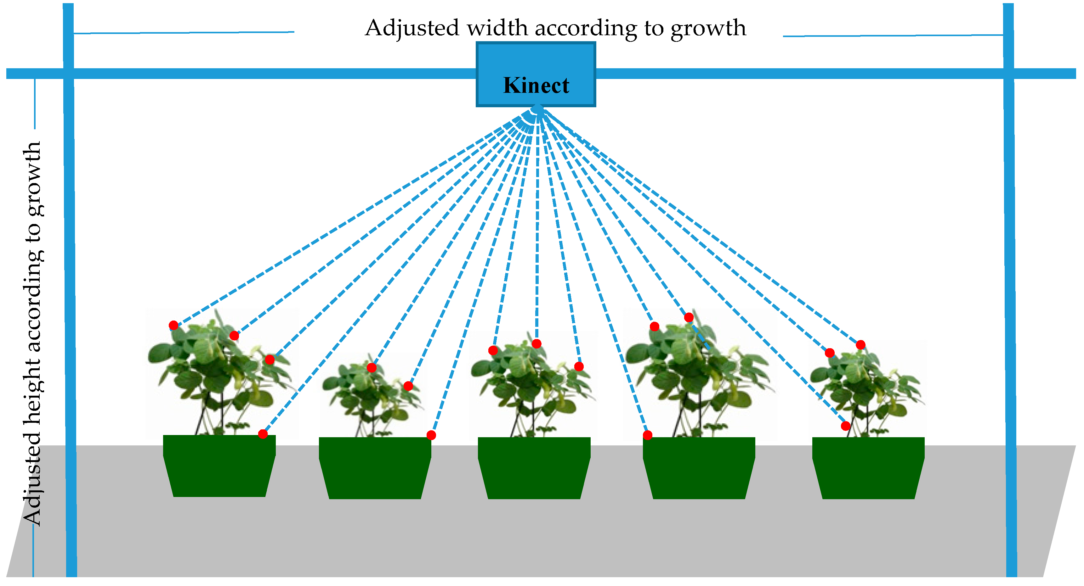
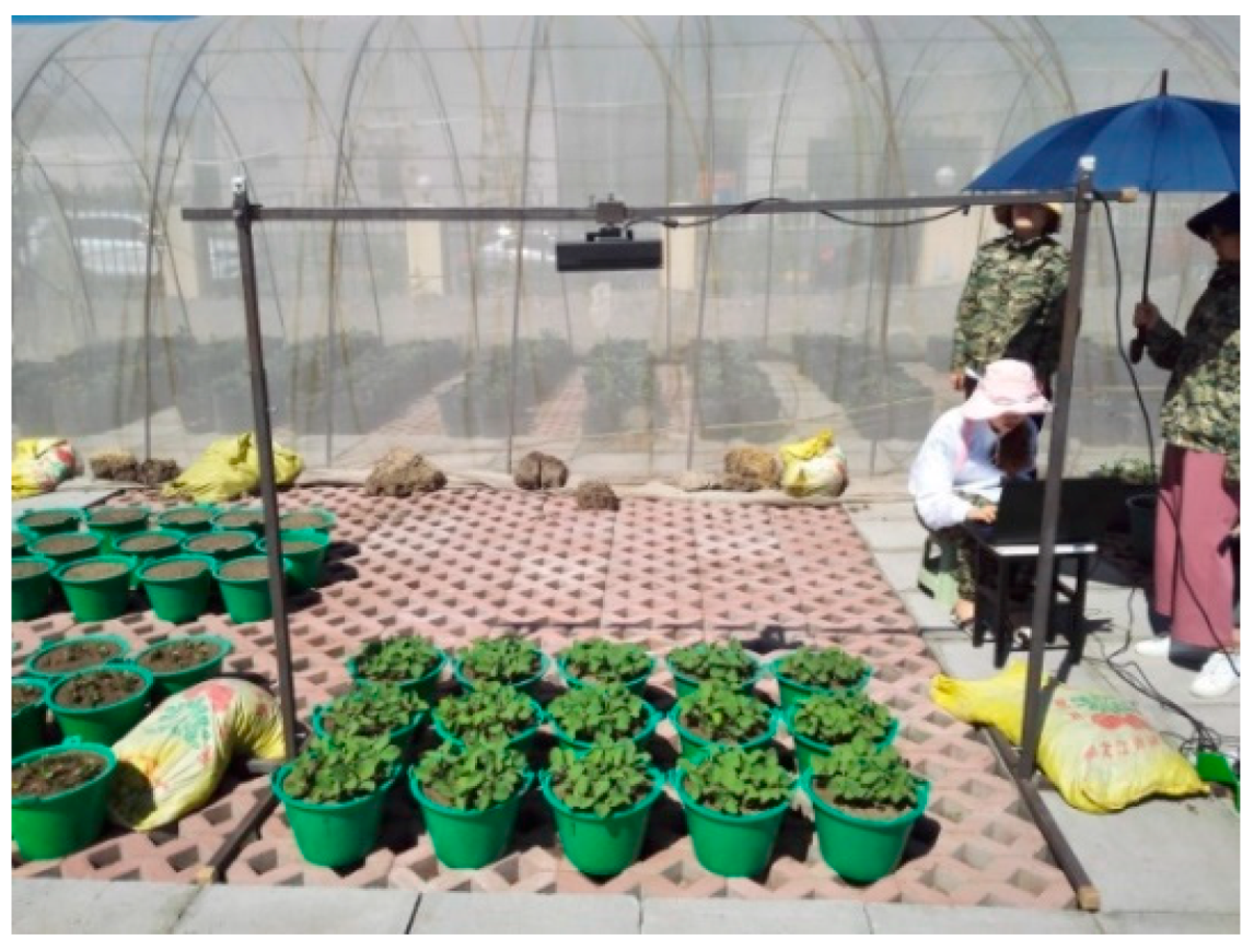
The proximal platform used for acquiring three dimensional (3D) data for soybean canopies was composed of three important parts: a Kinect v2 sensor, an iron frame allowing height and width adjustment and a data acquisition terminal.
The Kinect v2 sensor (Kinect-v2, Microsoft, Redmond, WA, USA), originally designed for natural interaction in computer gaming environments, can simultaneously acquire RGB images (1920 by 1080 pixels), depth images (512 by 484 pixels), and infrared images (512 by 484 pixels) of soybean canopies, with a field of view (FOV) of 70 degrees (H) by 60 degrees (V) and a measurement rate of 30 frames per second. With increasing distance, the accuracy decreases from a standard deviation (SD) of a few millimeters to approximately 40 mm, and the point-to-point distance decreases from 0.9 mm to 7 mm due to a FOV of 57 degrees (H) by 43 degrees (V) for Kinect V1 sensor [38], and reduced from 0.02 mm to 4 mm under a FOV of 70 degrees (H) by 60 degrees (V) for Kinect V2 sensor [39]. With the growth of soybean plants, plant height and canopy breadth gradually increase; thus, an iron frame with adjustable height and width was constructed to fix the Kinect senor, for the purpose of capturing the best 3D point cloud data of soybean canopies. The Kinect v2 sensor was installed on this frame and oriented vertically towards ground level (Figure 1). To acquire one group of soybean plants at the same time in different growth stages, the mounting height of the sensor ranged from 1500 mm to 2000 mm.
The mounting height plays a significant role in the proximal platform, since it affects the distance from the Kinect sensor to the measured distance points. Mounting height is also an important factor influencing the number of rows that can be simultaneously scanned by the Kinect sensor. Thus, based on the premise of ensuring distance accuracy, the Kinect sensor should simultaneously scan as many rows as possible without missing any plants, to increase the throughput of data acquisition.
The sensor was connected to a laptop (G50-45, Lenovo Technology Corporation, China) through a USB 3.0 interface and was controlled by in-house-developed software with store function, to obtain color images and 3D distance images simultaneously. Each group of plants was placed on the ground at the center of the sensor’ s FOV under natural conditions and was imaged at least six times for the calculation of phenotypic traits.
2.3. Overall Process Flow for Calculating Phenotypic Traits
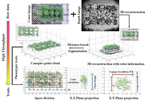
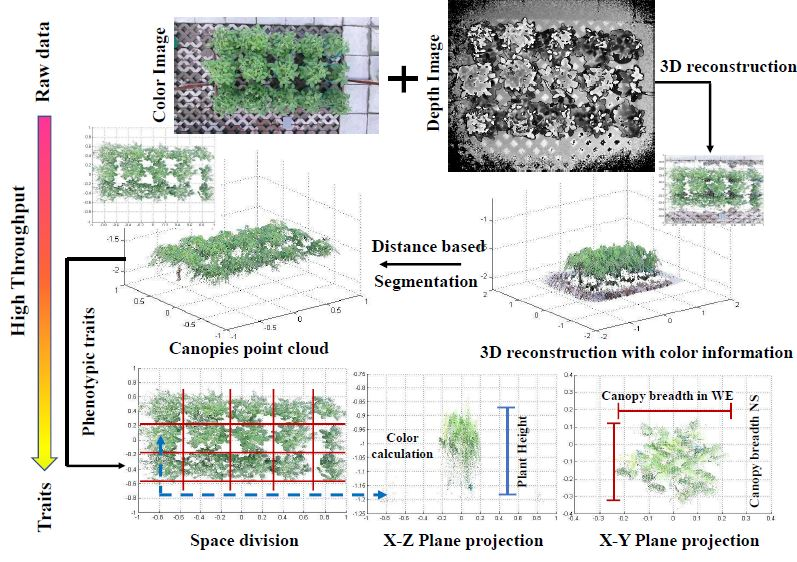
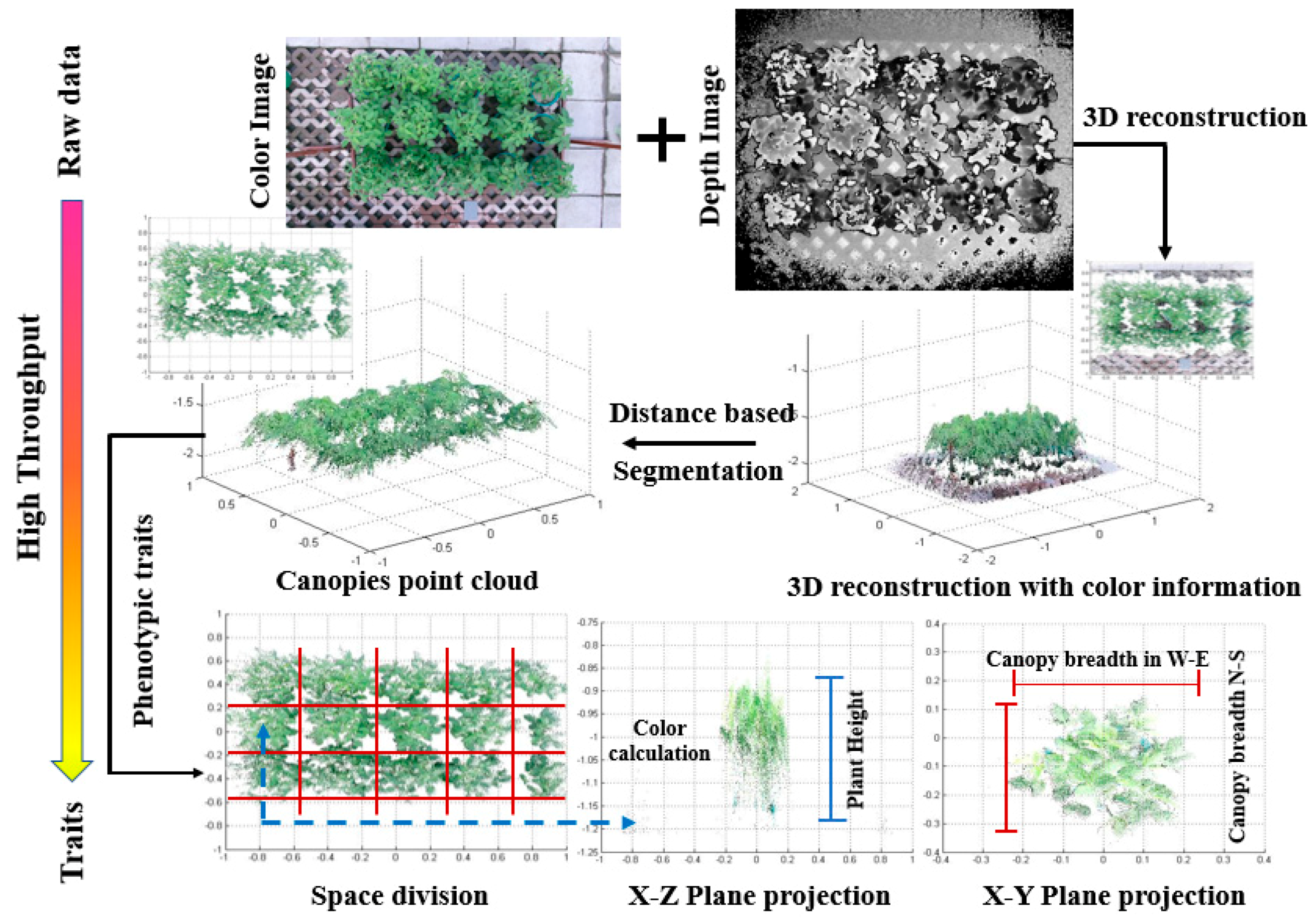
A technological process was developed to calculate the phenotypic traits of soybean plants by using the acquired color and depth images (Figure 2). The process included the following steps:
First, the color image and depth image of one group of soybean plants were collected by the Kinect sensor with the associated in-house-developed software. Second, the color image was registered in accordance with the R, G, and B values of a standard grad card. The raw depth and registered color images were then reconstructed to form colorized point clouds using a built-in function provided by the Software Development Kit (SDK) of Kinect v2. Additionally, soybean canopies were extracted from the complexed background based on distance information. Furthermore, a group of colorized 3D images of soybean plants were divided into fifteen single areas for 15 pots automatically according to spatial information. Finally, the reconstructed 3D plant points were used to calculate the following three phenotypic traits for each soybean plant: (1) the plant height (H) was the shortest distance from the upper boundary of the main photosynthetic tissues (excluding inflorescences) of a plant to the ground level [40]; (2) the canopy breadth, which consisted of two aspects: the width across-row (WAR) distance is the distance along the x-axis, while the width in-row (WIR) distance is the distance along the y-axis [30]; and (3) the color indices in the HSI color space.
These values above were also manually measured every week for reference. The 3D measurements and manual measurements were compared through simple linear regressions, and the determination coefficient R2 was used as an accuracy indicator.
2.4. Registration of Color Images
The color characteristic expresses the spectral reflection of visible light by soybean canopies. This important phenotypic trait can not only be used to extract target areas in image processing, but also reflects the growth of crops. Thus, it is essential to acquire true color information for soybean canopies. The quality of visible light imaging is greatly affected by the solar azimuth and light intensity under natural light conditions, which results in color distortion. Thus, for the purpose of expressing the true color of soybean canopies, color distortion must be registered before coloring the 3D cloud points using color information.
At present, most image processing software can register the appearance of color images; however, it only remains consistent in the visual sense, which is not suitable for occasions requiring quantitative analysis. In the application of color image recognition and analysis, an appropriate color correction algorithm must be sought to transform a color image obtained under certain light conditions to a color image under the predetermined standard light conditions, to guarantee the color constancy of the object under different light intensities. Recently, many methods have been used to eliminate or minimize the effects of light. The affine invariant theory and central moment analysis of color histograms were used to correct the effect of light on color information [41]. In addition, the black and white balance method was applied in color registration, through analysis of the color accumulation histogram of the reference plate of gray changes from black to white [42]. Although the above methods can effectively correct the color distortion problem, the algorithm is complex and time-consuming. In this study, a simple and effective color correction method was proposed based on the principle of three primary colors and color constancy.
A gray card (R = 128, G = 128, and B = 128), referenced for accurate exposure detection, was placed in the shooting scene and photographed together with the soybean plants. According to the good linear relationship of the photoelectric conversion of the photoelectric sensor, the mean R, G, and B values of the gray card were used as the reference for color registration. The correction coefficients of R, G, and B for the nonstandard image were obtained through comparing the reference values with the mean values of R, G, and B from the gray card of the nonstandard image, and the color of each pixel in the distorted color image was then registered according to the correction coefficients. This method is simple and requires little calculation without knowing the reflectivity of the subject and the channel response characteristics as well as the zero coordinates of the imaging system. The mean values of R, G, and B from the gray card of a nonstandard image were calculated as follows:
where , and were mean values of R, G, and B respectively, is the size of the color image and represents the coordinates of the pixels. In standard light conditions, the mean value of R, G, and B from the gray card should be 128, respectively; consequently, the registration coefficients of R, G, and B were , , , respectively. Thus, the R, G, and B value of each pixel after registration could be expressed as follows:
where, and represented the registered values of , and respectively.
The registration accuracy of the gray card represented that of the whole color image. The error of registration (E) for the gray card could be calculated through the changes in R, G, and B values after registration using Equations (7)–(9), which represented the registration error for the whole color image.
Thus, the color information of each pixel for the whole color image acquired in natural light conditions could be registered using Equations (4)–(6), which were further used for calculating color indices.
2.5. Calculation of Color Indices
Contrasting RGB and HSI color spaces, although the HSI color space is transformed from the RGB color space, it reflects the mechanism of color perception by the human visual system. Thus, the HSI color space was used to calculate color indices to express the color characteristics of soybean canopies.
A reconstructed 3D image with color information was investigated in the HSI color space. The color distortion affected by light was registered prior to RGB decomposition, in which the R, G, and B channels of the image were extracted. Color characteristics, including H, S, and I components, were obtained from the R, G, and B values of the 3D soybean canopy. All of the points in the 3D point cloud were traversed to calculate the H, S, and I values. We applied the following scheme to obtain the color indices from the HIS color space, which were used to express the color characteristics.
where , , and are the three color indices and , , and represent the values of the H, S, and I channels at 3D coordinates (x, y, and z), respectively. The efficiency of the calculation results depended on the accuracy of color registration.
2.6. Calculation of Plant Height
Plant height in the single plant layout may be more indicative of plant growth and development. In the agronomy research field, the plant height of soybean plants is conventionally measured using rulers or a handheld laser rangefinder. However, these manual measurement methods are time-consuming and labor-intensive and are therefore not suitable for high-throughput measurements. In addition, the geometric structure of soybean plants may be much more complex than that of other major field crops, such as rice and wheat. Therefore, a dense and valid 3D point should be acquired to ensure that the highest positions of soybean canopies are scanned by the Kinect sensor within an effective shooting range. To account for ambient effects, such as light intensity and wind power, the depth accuracy of the Kinect v2 camera was evaluated by measuring plant height in natural conditions.
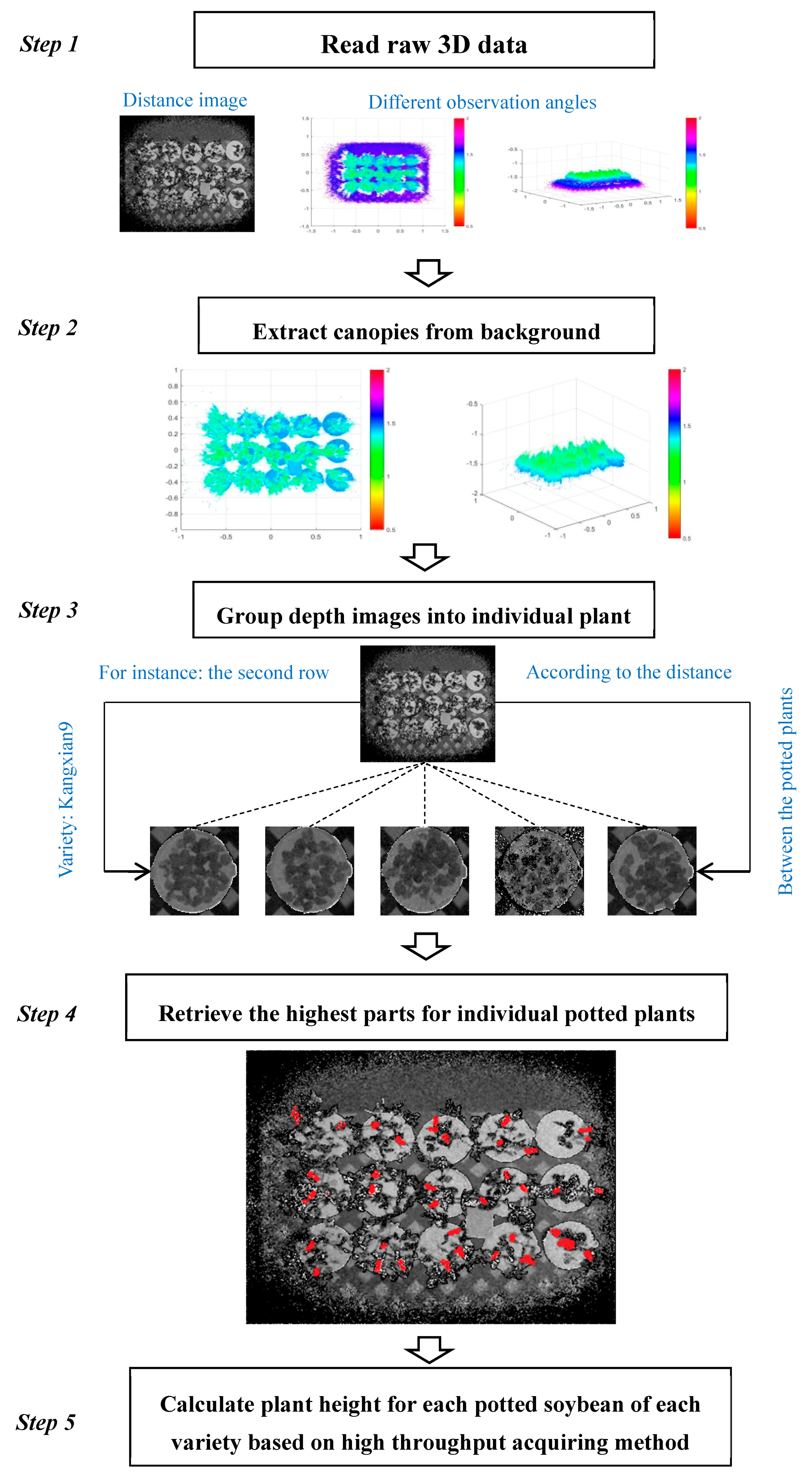
An algorithm with a detailed flowchart was developed to calculate the plant height of potted soybean plants by using the acquired depth images (Figure 3). The algorithm included five steps:
First, the raw 3D distance images were read by a program developed in MATLAB (MATLAB 2015b, The Math-Works Inc., MA, USA). The X, Y, and Z coordinates of all the 3D points were stored in a matrix. To distinguish canopies and background, different colors were assigned to 3D points according to distance information with the color bar in the MATLAB environment.
Second, point clouds of soybean plants may contain irrelevant objects, such as the ground surface and weeds. Therefore, it was necessary to extract the soybean canopy from background objects. Point clouds were rasterized to depth images, so the pixels of the soybean canopies were differentiated from those of the background in the depth images by using spatial information, including height and position.
Third, individual potted soybean plants were successively separated from a group image containing 15 potted soybean plants, in accordance with the diameters of pots and the intervals between the pots. It should be noted that the intervals were also variable values: as the canopy grows, the interval must be manually increased to prevent overlap of adjacent canopies.
Fourth, the highest parts of individual potted plants were retrieved for further calculation of plant height. The highest point was defined as an average height value of 50 pixels that exhibited the 50 minimum values in a valid distance range. The distance values were sorted from high to low in the range of X and Y coordinates for each potted plant separated in the third step, and the top 50 highest points in the sequence were selected to generate the height profiles.
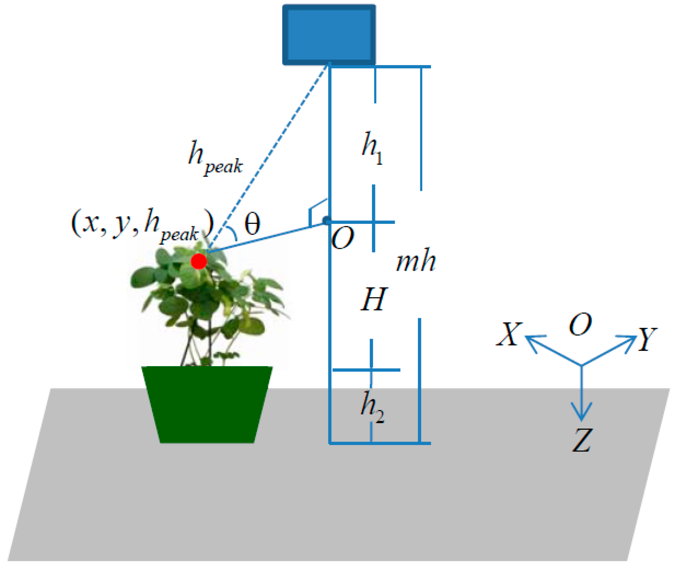
Fifth, one of the groups of potted soybean plants was used to describe the calculation principle of plant height. The calculation method is demonstrated in Figure 4. The average value of the selected points in the fourth step was used to calculate the plant height for each potted soybean plant of each variety using Equations (13) and (14).
where is the coordinate of the highest point, is the distance from the Kinect sensor to the highest point , is the vertical distance from the Kinect sensor to the highest point , is the height of pot, is the mounting height of the Kinect sensor, and is the plant height.
2.7. Calculation of Canopy Breadth
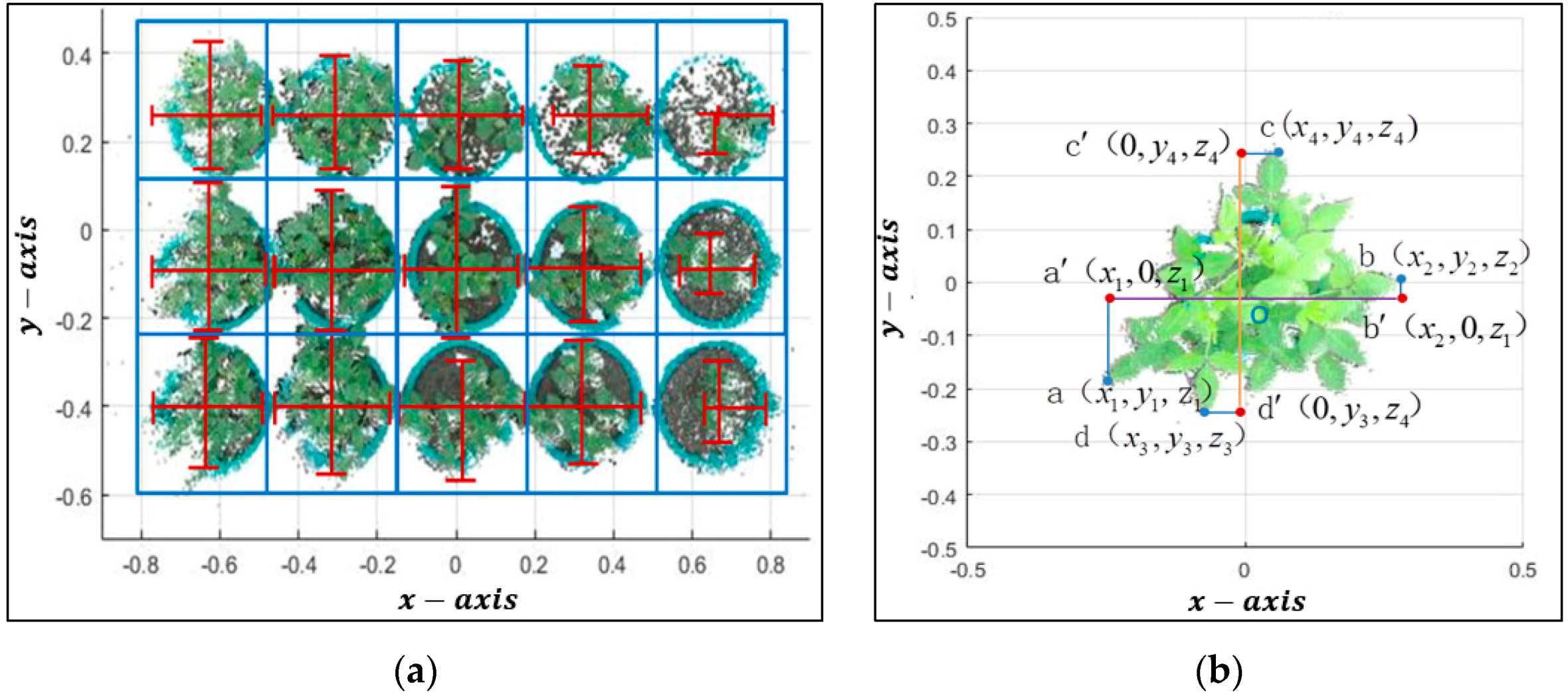
Canopy breadth is not only consistently related to the ratio of the leaf area per plant, but also is an essential factor determining the light distribution [43]. For canopy breadth, the point cloud of a soybean canopy was segregated into three segments across the row direction and five segments in the row direction. The maximum length in each direction was calculated in each segment (Figure 5a).
Based on the division of group canopies in step 3 of Section 2.6, the coordinates of the boundary points for each individual plant were recorded in the row direction and across the row direction (Figure 5a). Points a and b were the 3D boundary points in the row direction, which were projected onto X axis of the X–Y plane in the same horizontal plane. Points c and d were the 3D boundary points across the row direction, which were projected onto the Y axis of the X–Y plane (Figure 5b). The canopy breadth was calculated using Equations (15) and (16).
where DIS represents the distance between two boundary points in each direction, and are the projection points on the X axis of points a and b, respectively, and and are the projection points on the Y axis of points c and d, respectively For inclusion in the same horizontal plane, the z value of was adjusted to from , and the z value of was adjusted to from .
3. Results
3.1. Accuracy of Color Registration
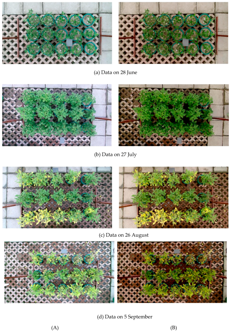
Soybean canopy data were acquired under natural light conditions (Figure 6), including sunny or cloudy days, and wind speeds less than 0.9 m/s. Light intensity and mounting height of Kinect at the time of data collection were listed in Table 1. Although vertical shooting mode can minimize the impact of light on the imaging effect of color images, distortion still exists in color images and affects the expression of the true spectral reflectance. How accurately the color distortion of soybean canopies is registered when captured under natural light conditions is critical for accurate determination of color characteristics. For the purpose of registering color distortion, the gray card used as a reference was placed anywhere within the shooting area. The registration process was performed using the scheme presented in Section 2.4. Color images were captured during growth stages in natural light conditions with a light intensity lower than 1000 Lux. For illustration of the registration effects, the color images obtained on 28 June, 27 July, 26 August, and 5 September were registered; these dates represented the branch period, flowering period, scabby period, and seed-filling period, respectively (Figure 7).
To verify the effectiveness of the registration algorithm, the area of the gray card was extracted for each image using Photoshop software (Version: CS6.0). In addition, the mean values of the R, G, and B bands of the gray card in color-distorted images and color-registered images were calculated. Table 1 indicates that the mean values of R, G, and B of four color-distorted images under natural light conditions presented in Figure 7A deviated from the reference values to a large extent, due to effect of the light intensity, while the mean values of R, G, and B of the four color-registered images in Figure 7B after registration were very close to reference values, which proved the high registration accuracy of the color for soybean canopies. The maximum error of registration for R, G, and B bands in the dataset was 1.26%, 1.09%, and 0.75%, respectively. The results demonstrated the effectiveness of the registration algorithm with respect to color constancy and its usefulness for further calculation of color indices (Table 2).
3.2. Extraction of the Soybean Canopy Based on 3D Point Cloud
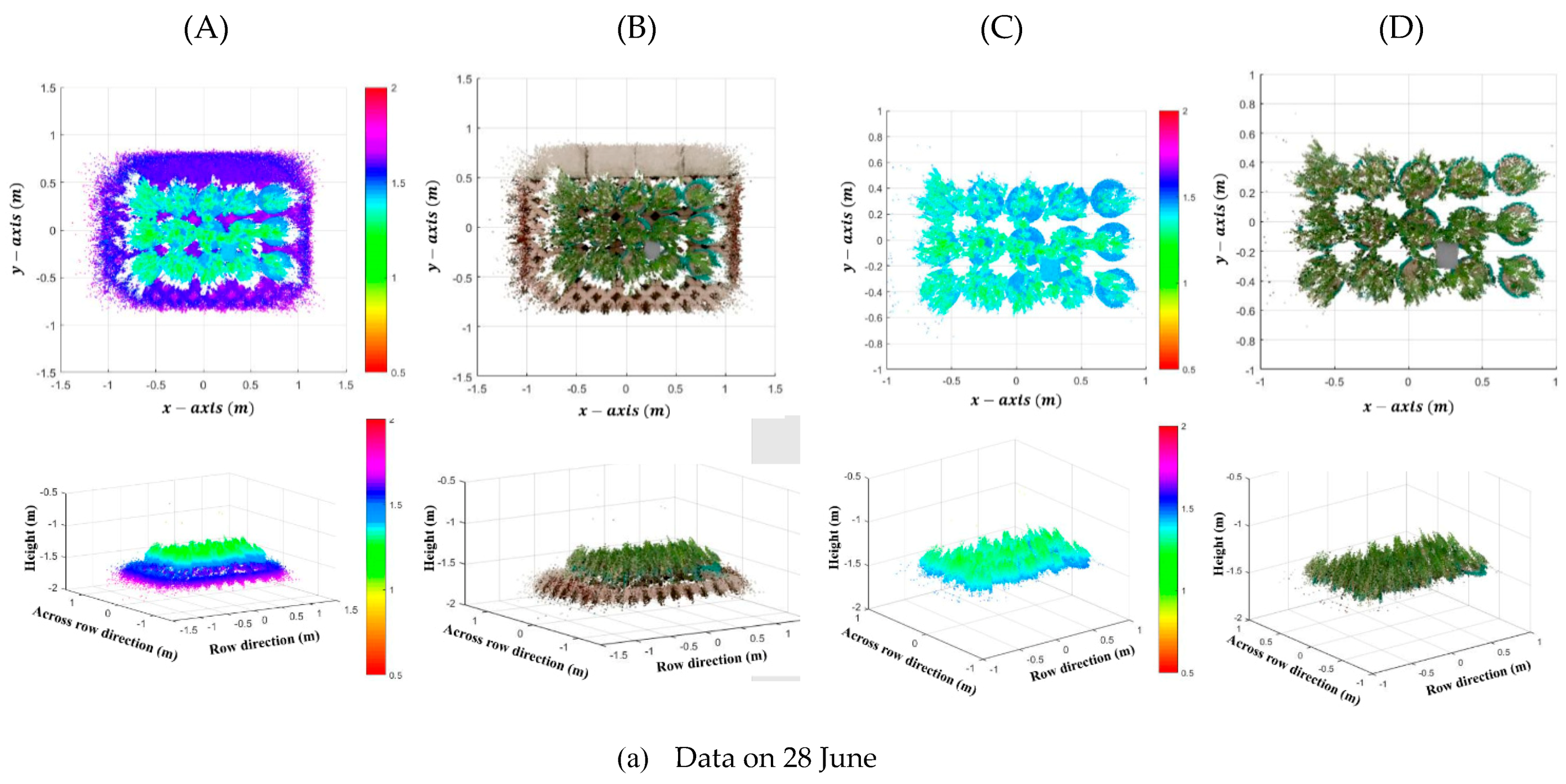
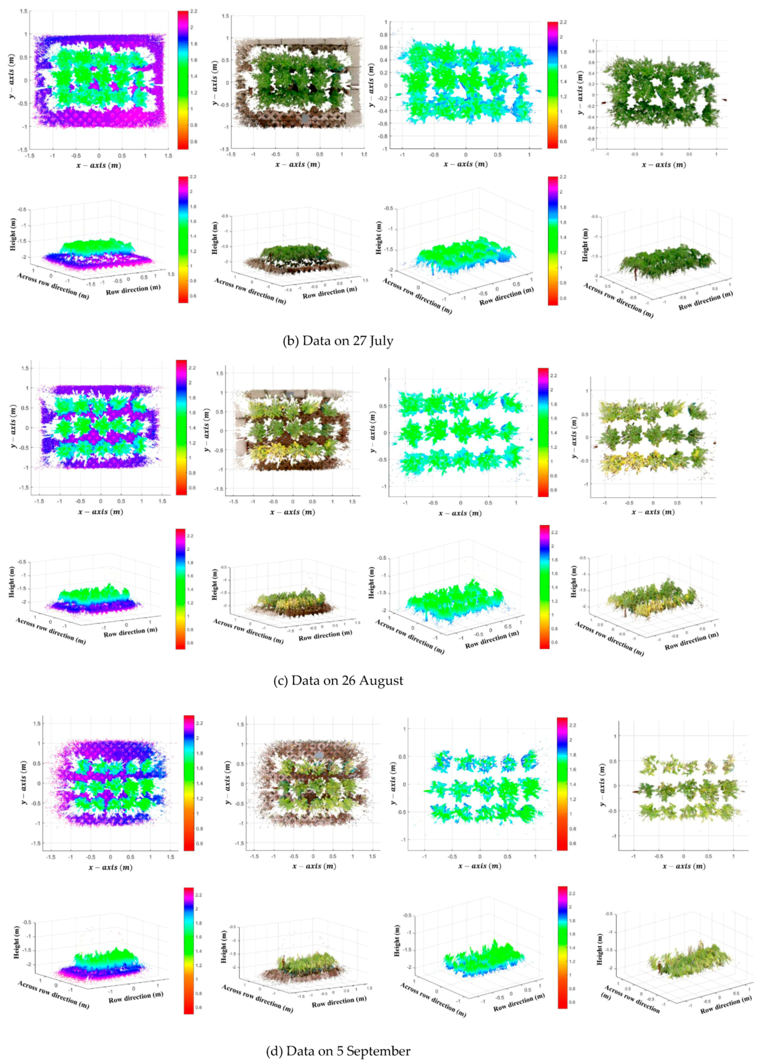
For illustration purposes, the raw data acquired on 28 June, 27 July, 26August, and 5 September were selected to demonstrate the reconstruction results. The raw depth and corresponding registered color images could be reconstructed to generate point clouds with color information using a built-in function provided by the Kinect v2 SDK sensor. An accurate 3D reconstruction effect could be achieved due to exact calibration between the color camera and the depth camera using this consolidation program.
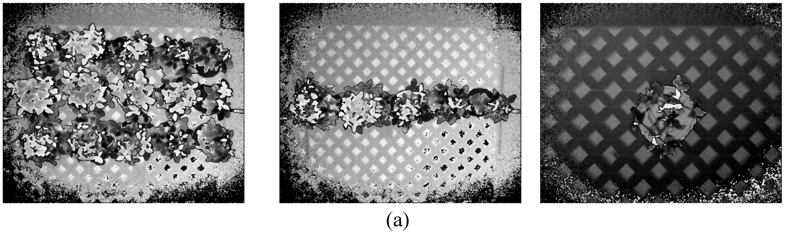
Soybean canopy extraction strongly affected the accuracy of trait calculation. In particular, the removal of background items, such as the ground and pots, significantly impacted the values of the extracted geometric and color traits. The raw distance information of the soybean canopies and background could be expressed using the raw distance images (Figure 8A). Colorized 3D points of raw data could be clearly formed through fusion of the 3D distance information and the registered color information (Figure 8B). For the purpose of extracting 3D points and color information, the adjusted threshold area of the distance was set to remove the background according to different growth stages. Threshold area Z was (1.30 m < Z < 1.45 m), (1.30 m < Z < 1.70 m), (1.30 m < Z < 1.80 m), and (1.30 m < Z < 1.90 m) at the branch period, flowering period, scabby period, and seed-filling period, respectively. Thus, the 3D distance information of the soybean canopies could be exactly segmented from the raw data in accordance with the threshold indicated above (Figure 8C), and the color information registered on 3D distance points could be simultaneously extracted (Figure 8D). The validity of the extraction of the soybean canopy could be evaluated based on the calculation accuracy for phenotypic traits.
3.3. Accuracy of Plant Height
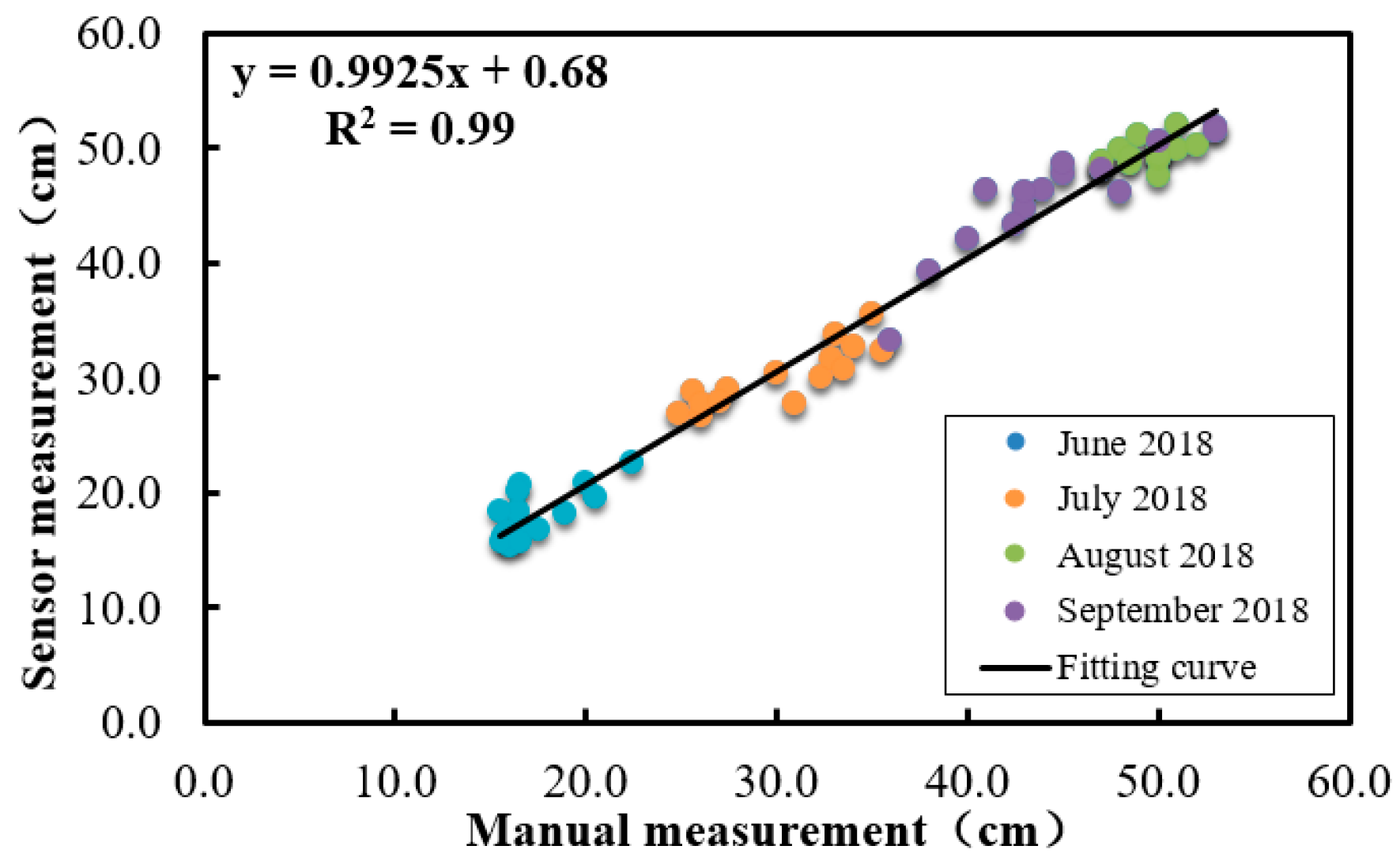
Sensor measurements of plant height at four months were subjected to comparison with the ground truth. Manual measurements and sensor measurements were taken every seven days on average; thus, each month included four measurements. There were total 60 sets of data after averaging the measurement values for each month. For the average plant height of each potted soybean plant in each month, the sensor measurements were strongly correlated (adjusted R2 = 0.99) with the manual measurements (Figure 9), and root mean squared error (RSME), mean relative error (MRE), and mean absolute error (MAE) were 1.92 cm, 5.1%, 1.58 cm, respectively (Table 3). Height increased with the growth stage except in the seed-filling period. In the canopy development stage, the transpiration capacity of plant leaves was increased, and leaf morphology and size gradually stabilized to receive more sunlight for photosynthesis. Therefore, at the canopy growth stage, the upper leaves of the canopy occluded the lower ones, resulting in minor variation in calculation of plant height in the seed-filling period. In addition, the soybean canopies encountered continued major rains, resulting in nutrient loss from the soil and were in turn infested with insect pests in the seed-filling period during the data collection period, leading to falloff of the upper leaves. Thus, some height measurements from this period were lower than their counterparts in the other three periods.
3.4. Accuracy of Canopy Breadth
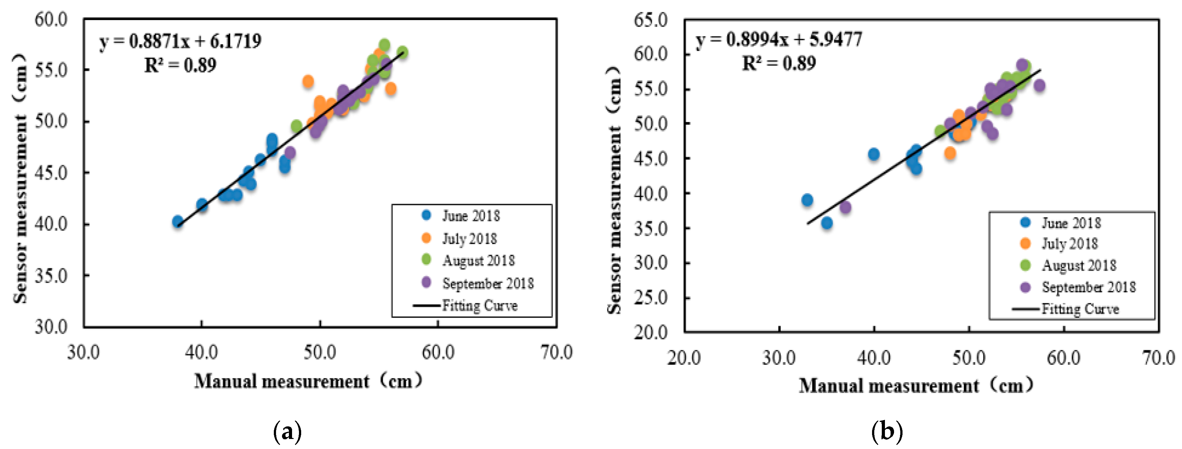
Overall, the average canopy breadth determined from the sensor measurements was in good agreement with the ground truth (Figure 10). Values of RSME, MRE, and MAE for canopy breadth in the W–E direction were 1.23 cm, 2.4%, and 0.9 cm respectively, and 1.85 cm, 2.9%, and 1.44 cm for canopy breadth in the N–S direction, respectively (Table 3). Similar to the variation tendency of plant height, the sensor measurement values of canopy breadth, including the WAR and WIR directions, gradually increased in the branch, flowering, and scabby periods and decreased in the seed-filling period. In the calculation of canopy breadth, there were three additive error sources. First, in addition to the weather effects, the overlap of canopy edges made them undetectable to the Kinect sensors in terms of growth. Second, leaves began to shrink and fall off, resulting in a reduction of canopy size. Third, from the device itself, the Kinect sensors could not capture depth information for an occluded object from a single vertical view, leading to partial loss of data.
3.5. Calculation of Color Indices
A crucial focus of this section is to propose a practical method for reflecting health status that provides quantified color characteristics to crop experts for diagnosing the diseases and nutrient conditions of soybean plants.
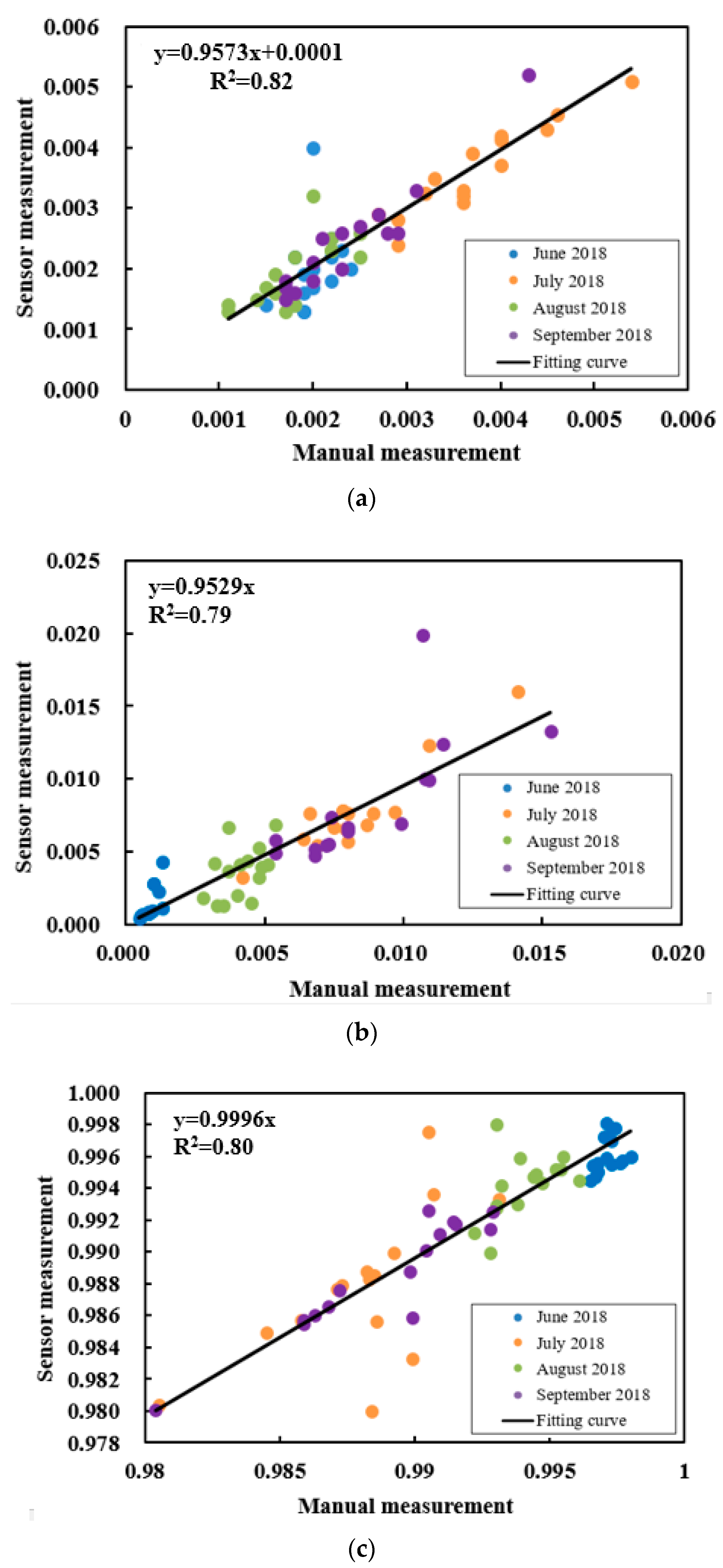
In this research, the R, G, and B values of each 3D point cloud were extracted from the reconstructed soybean canopies and converted to HSI color space. Color indices, including H, S, and I, were calculated according to Equations (10)–(12), respectively. Meanwhile, color indices calculated for canopies that extracted from 2D color images using photoshop software were regarded as manual measurement values for comparing with the counterpart calculated from 3D canopies. Figure 11 showed that sensor measurement values of color indices h, s, and i were strongly correlated with manual measurement values with determination coefficient R2 of 0.82, 0.79, and 0.80 respectively. Values of RSME, MRE, and MAE were 0.0004, 7.8%, and 0.0003 for color index h, 0.0018, 8.5%, 0.0013 for color index s, and 0.0022, 7.1%, 0.0013 for color index i, respectively (Table 3). The calculation accuracy of the color indices depended on the effectiveness of color registration as described in Section 2.4. In addition, this good linear regression results further verified the effectiveness of color information reconstructed to 3D canopies.
3.6. Comparison of Phenotypic Traits for Different Varieties
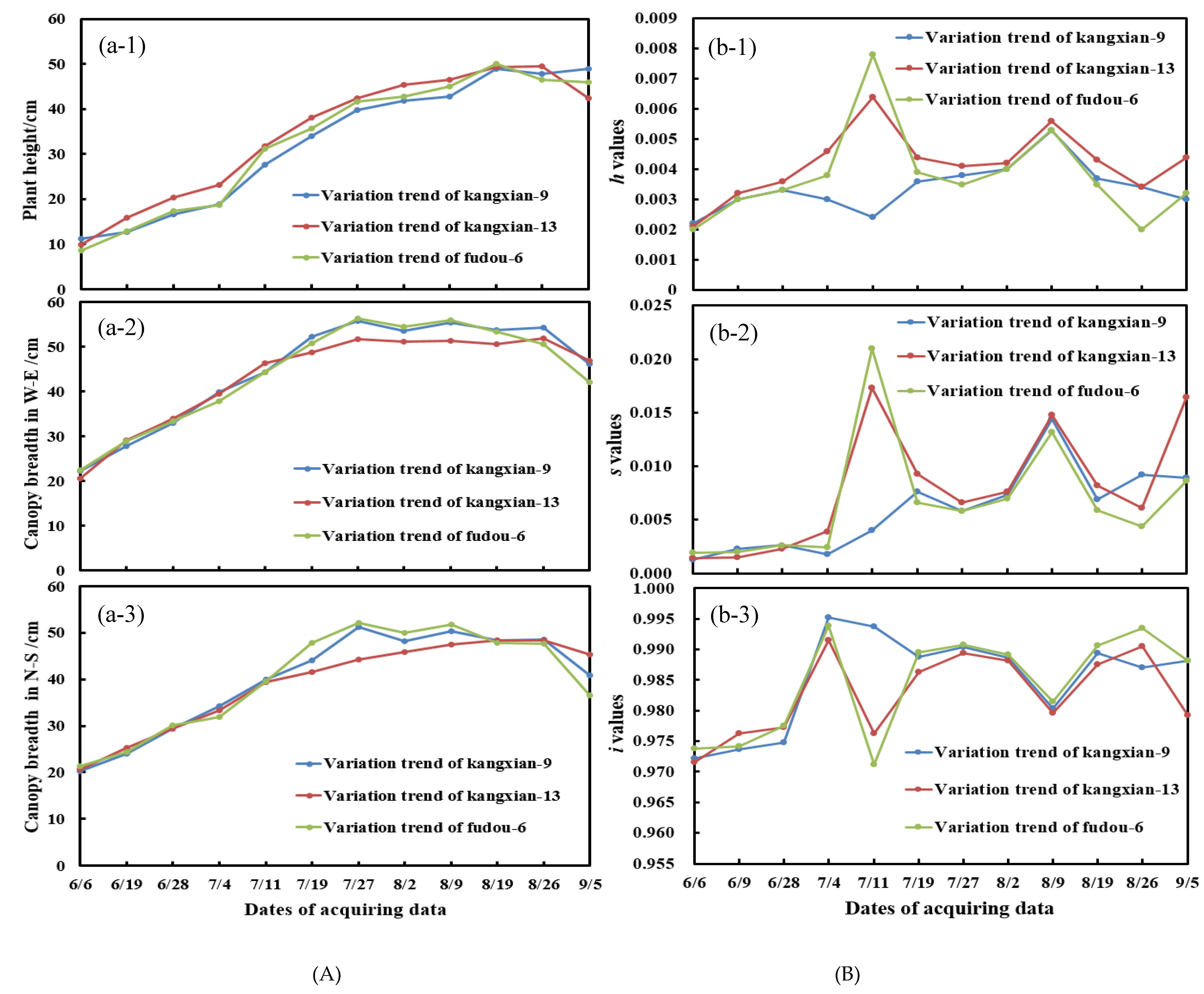
Phenotypic traits for three different varieties based on time series were analyzed; plant height and canopy breadth increased gradually under the same conditions of cultivation and management. The variation trend of phenotypic traits are determined by the genotype of crop varieties. Kangxian 13 is a compact variety with tall plant height and narrow canopy breadth. On the contrary, Kangxian 9 and Fudou 6 are open scattered varieties with relatively short plant height and relatively wide canopy breadth. Thus, the average plant height of Kangxian 13 was higher than the other two varieties, and the average canopy breadth at scabby period was lower than the other two varieties. There was no obvious difference between varieties of Kangxian 9 and Fudou 6 (Figure 12a-1). For canopy breadth, they grew at almost the same height from 6 June to 11 July (branch period and flowering period), while variety of Kangxian 13 grew slower than the others either in W–E direction or N–S direction from 11 July to 26 August (scabby period and early seed-filling period). In addition, on September 5th (seed-filling period), the canopy breadth of Kangxian 13 was wider than that of Kangxian 9 and Fudou 6, Fudou 6 had the lowest canopy breadth of all (Figure 12a-2 and a-3).
Although variation of color indices was much more dramatic than the counterpart of plant height and canopy breadth, they also showed certain regularity. From 6 June to 28 June (branch period), values of H, S, and I showed the same variation with increasing tendency. However, color indices change as the soybean plants grow, values of H, S, and I displayed different variation trend. For color index h, the variation trend of Kangxian 9 was the opposite to that of Kangxian 13 and Fudou 6 from 28 June to 2 August (scabby period and early seed-filling period), while these three varieties showed similar variation trend from 2 August to 5 September (seed filling period). The range of variation was [0.021,0.064], [0.0022,0.0053], and [0.002,0.0078] for Kangxian 13, Kangxian 9, and Fudou 6, respectively, (Figure 11b). For color index s, Kangxian 13 and Fudou 6 presented similar variation trend from 6 June to 26 August, while Kangxian 9 displayed reverse trend comparing to Kangxian 13 and Fudou 6 from 19 August to 5 September. The range of variation for index s was [0.0014,0.0173], [0.0013,0.0144], and [0.0019, 0.0132] for Kangxian 13, Kangxian 9, and Fudou 6, respectively (Figure 12b-2). For color index i, except the stage from 19 August to 5 September, variation trend of Kangxian 9 was similar to that of Kangxian 13 and Fudou 6, with variation range of [0.9715,0.9915], [0.9722, 0.9952], and [0.9712, 0.9938] for Kangxian 13, Kangxian 9, and Fudou 6, respectively (Figure 12b-3).
Figure 12 illustrates that in the whole growth stages of crop plants, the degree of changes in the values of phenotype traits occurred as a result of the changes of composition such as Chlorophyll, nitrogen, or moisture contents [44,45]. These phenotypic traits and corresponding variation trends will further help breeders carry out breeding and testing of soybean plants.
Figure 12a shows that canopy structure tends to be stable in the later period (from 19 August 2018 to 5 September 2018) of soybean growth stages. Thus, calculated results of 19 August 2018 were selected for statistical analysis. In this study, there was no significant difference about plant height and canopy breadth between Kangxian 9, Kangxian 13, and Fudou 6 (Table 4). In addition, there was also no significant difference between the three varieties about color indices h and i under the same fertilizer and water management, while there was clear distinction about color index s which can be used for distinguish these three varieties. Thus, the proposed methods had strong universality, being suitable for calculating plant height, canopy breadth, and color characteristics of soybean plants effectively and providing reasonable description of phenotypic traits for breeders.
4. Discussion
The application of a Kinect sensor in the acquisition of soybean canopy information in natural light conditions could reduce costs and increase the utilization of imaging techniques in the field of phenotypic research, benefitting the plant science community [46,47]. The image acquisition platform has been demonstrated to be capable of using Kinect sensor for data collection in a high-throughput fashion under natural light conditions. In this study, a group of soybean canopies in three rows and five columns was simultaneously collected for geometric and color calculation. This relatively high throughput was a major benefit of the proximal platform compared to manual measurements and the side view scanning method utilized in related research [48,49]. Although high accuracy has been achieved based on the acquisition system and calculation method proposed in this paper, it still needs to be improved further.
4.1. Analysis of the Experimental Results
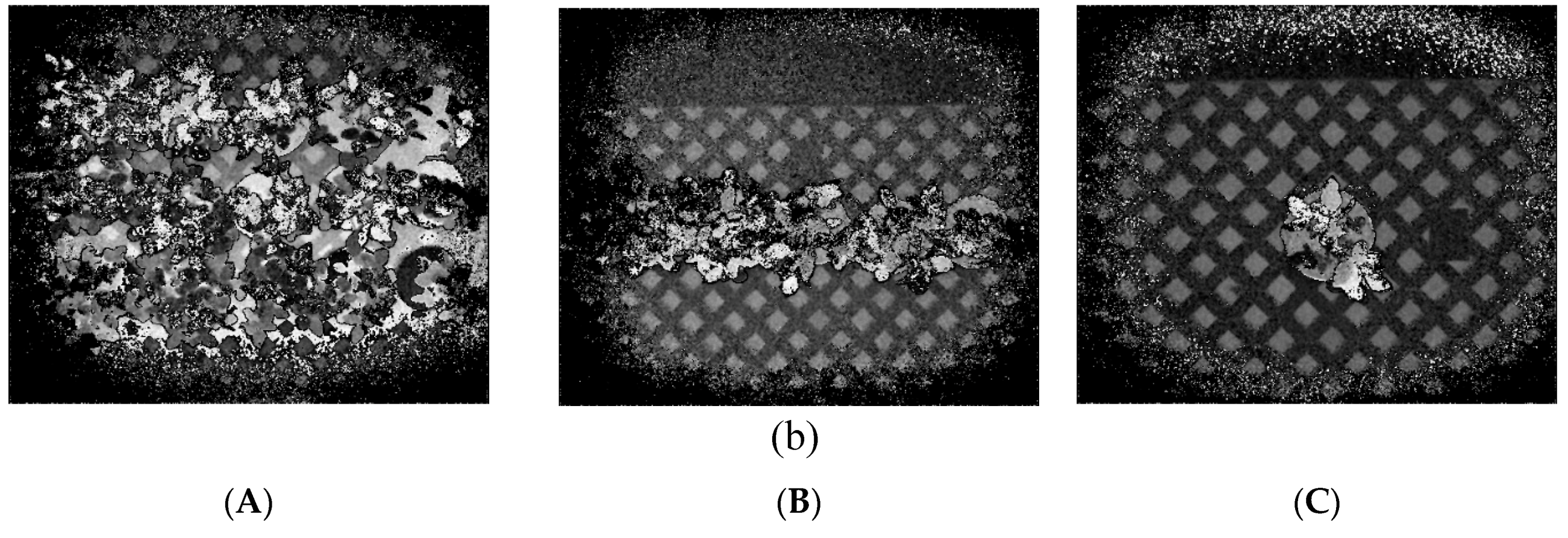
The geometric traits calculated via the image processing method were positively correlated with the manual measurements. One-to-one comparison of geometric traits resulted in R2 values of 0.99, 0.89, and 0.89 for plant height and canopy breadth in the W–E and N–S directions, respectively. Although the experiments were conducted under natural light conditions, it would be better to acquire data under shaded conditions in practice, such as on cloudy days or using shading structures. Due to the limited performance of the depth sensor, the infrared emitters, and the surfaces’ materials, which are sensitive to ambient light, especially sun light, the 3D depth information changes over time. Even if the Kinect sensor is stationary, a 3D point will vary by several millimeters [39]. Thus, shaded conditions can avoid changes of external light to a large extent and potentially keep the quality of a 3D point cloud. For phenotyping analysis of cotton plants, shaded components were designed for the Kinect sensor on tractor to guarantee the quality of 3D data [50,51]. In terms of imaging effects, data acquisition under natural conditions with a light intensity lower than 500 Lux could result in a better image quality, while severe noise will occur in distant images acquired under natural conditions with a light intensity of more than 1000 Lux (Figure 13). The degradation of point cloud quality was mainly reflected in the edges of the leaves, leading to a reduction in the number of valid point clouds. This phenomenon has been demonstrated by a previous study that indicated that no more than a half of points can be accurately acquired by Kinect sensors under strong light conditions, ultimately resulting in a decrease in the image acquisition throughput [52]. This phenomenon was the reason that the calculation accuracy for canopy breadth was lower than that of plant height, due to missing edge points of leaves. Thus, it is better to acquire data for soybean canopies in shady locations under natural conditions.
For color images, light intensity can have a great impact on the imaging effect; however, this color distortion can be largely eliminated by the algorithm proposed in Section 2.4. However, the accuracy of color registration depended on the quality of the gray card. Dust and prolonged exposure to sunlight cause discoloration that affects the accuracy of the gray card as a reference. Therefore, a new gray card must be used for each data acquisition to ensure high registration accuracy for the entire color image.
4.2. Limitation and Scalability of the Acquisition System
The present study verifies the ability to use Kinect v2 and proposes algorithms to calculate the plant height, canopy breadth, and color indices of soybean plants in a rapid and accurate fashion. However, two factors constrain the performance of the proposed approach. First, Kinect sensors are sensitive to strong light intensities, which limits the data acquisition time. Second, Kinect for Windows SDK 2.0 introduced the Kinect Fusion function that enables us to use Kinect for Windows sensors to perform 3D geometric reconstruction of real scenes, and currently supports exporting 3D data formats such as. Obj and. STL [53]. In addition, it also enables real-time 3-D modeling of objects on Graphic Processing Unit (GPU)-accelerated machines [54]. High speed and convenience is the biggest advantage of the SDK 2.0 compared to traditional 3D modeling method [55]. However, reconstruction of colorized 3D cloud points based on fusion function using Kinect SDK must be executed on a computer running an operating system of Windows 8 (or later) connected to the Kinect v2 camera, which might restrict the throughput of 3D reconstruction [52]. This limitation can be addressed using in-house-developed synchronous acquisition software through registration between depth and color images. Kinect v2 is not a new device for calculating phenotypic traits. However, the present study demonstrated that Kinect v2 can provide accurate geometric trait measurements, which creates new opportunities for field-based soybean plant phenotyping. In particular, the state-of-the-art, high-throughput phenotyping platform for soybean plants can be further improved with a high-clearance tractor equipped with a real-time kinematic GPS in field conditions. It should be noted that only depth and color information were utilized in the present study, while other information was not taken full advantage of, which leaves a large space for development. For instance, obtaining the ROI coordinates and the position of an object within the SDK will be useful for the identification of internodes for the further calculation of branch angles. In addition, according to the imaging principle [56], if the output of electric signal of imaging components such as CCD or CMOS is too strong, the phenomenon of “oversaturation” will appear [57,58]. Thus, avoidance of acquiring color images in strong light is one of the effective ways to overcome the oversaturation problem.
4.3. Future Work
The plant height, canopy breadth, and color indices of the three genotypes of soybean plants were calculated using Kinect v2 and the approach proposed in this study. However, from a plant science and breeding perspective, a promising approach should be considered in future work to increase the throughput at larger observational scales by capturing multiple soybean plants in group mode and measuring other phenotypic traits, such as stem diameter, branch angles, and the leaf area index, as much as possible. These traits could be used to assist plant breeders in the selection of soybean genotypes. For example, they are used as indicators to identify early maturing soybean cultivars that can reduce yield losses due to diseases [59,60] and insect–pest complexes [61]. From a technical perspective, geometric traits can also be accurately measured using other imaging sensors, such as light detection and ranging (LIDAR) sensors, and color indices can be accurately acquired using a near-infrared spectroscopy camera.
In addition to the static traits indicated above, dynamic traits, such as growth rates [51], will be considered in our future work, which could provide information about the growth behavior of soybean plants throughout their growth stages. The detection of such variations in growth rates might permit the identification of genes controlling soybean plant growth patterns or the selection of soybean genotypes with strong resistance for high production or harvesting strategies.
5. Conclusions
The synchronous acquisition platform and data processing algorithms described herein provide an inexpensive solution for accurately quantifying the geometric and color traits of soybean canopies under natural light conditions. The main achievements of this study are summarized as follows:
(1) To measure plant height, canopy breadth, and color indices, a proximal platform equipped with a Kinect v2 camera was built as a synchronous acquisition system for the high-throughput acquisition of color and depth information for soybean canopies in groups.
(2) The distortion phenomenon of color images was recognized prior to reconstruction of the colorized three-dimensional structures of soybean canopies in accordance with the principle of three primary colors and color constancy. For the R, G, and B bands of gray card, the maximum errors of registration were 1.26%, 1.09%, and 0.75%, respectively, which demonstrated the effectiveness of the registration algorithm. Color indices were further calculated in the HSI color space.
(3) Colorized 3D soybean canopies were reconstructed and extracted from the background. Algorithms for plant height and canopy breadth were proposed considering a group of soybean plants. Correlation analysis between the sensors and manual measurements yielded R2 values of 0.99, 0.89, and 0.89 for plant height and canopy breadth in the WAR and WIR directions, respectively, in addition, R2 values for color indices H, S, and I were 0.82, 0.79, and 0.80 respectively, confirming the usefulness of applying the synchronous acquisition platform and data processing algorithms in phenotypic studies.
(4) Statistical analysis indicated that there was significant difference about color index s between Kangxian 9, Kangxian 13, and Fudou 6, while there was no obvious distinction about plant height and canopy breadth as well as color for indices h and i.
Author Contributions
H.G., X.M. and G.L. conceived and designed the experiments; J.F. and K.Z. performed the experiments and acquired the 3D data of soybean canopy; X.M., J.F. and K.Z. calculated plant parameters; S.Y. directed the soybean planting; X.M. wrote the paper.
Funding
This study was funded jointly by National Natural Science Foundation of China (31601220), Natural Science Foundation of Heilongjiang Province (QC2016031), China Postdoctoral Science Foundation (2016M601464), and Support Program for Natural Science Talent of Heilongjiang Bayi Agricultural University (ZRCQC201806).
Acknowledgments
The authors would like to thank the two anonymous reviewers, academic editors for their precious suggestions that significantly improved the manuscript.
Conflicts of Interest
The authors declare no conflict of interest.
References
- Tilman, D.; Balzer, C.; Hill, J.; Befort, B. Global food demand and the sustainable intensification of agriculture. Proc. Natl. Acad. Sci. USA 2011, 108, 20260–20264. [Google Scholar] [CrossRef] [Green Version]
- Eriksson, D.; Brinch-Pedersen, H.; Chawade, A.; Holme, I.; Hvoslef-Eide, T.A.K.; Ritala, A. Scandinavian perspectives on plant gene technology: Applications, policies and progress. Physiol. Plant. 2018, 162, 219–238. [Google Scholar] [CrossRef]
- Halewood, M.; Chiurugwi, T.; Sackville Hamilton, R.; Kurtz, B.; Marden, E.; Welch, E.; Michiels, F.; Mozafari, J.; Sabran, M.; Patron, N.; et al. Plant genetic resources for food and agriculture: Opportunities and challenges emerging from the science and information technology revolution. New Phytol. 2018, 217, 1407–1419. [Google Scholar] [CrossRef]
- Chelle, M. Phylloclimate or the Climate Perceived by Individual Plant Organs: What Is It? How to Model It? What For? New Phytol. 2005, 166, 781–790. [Google Scholar] [CrossRef] [PubMed]
- Hawkesford, M.J.; Lorence, A. Plant phenotyping: Increasing throughput and precision at multiple scales. Funct. Plant Biol. 2017, 44, v–vii. [Google Scholar] [CrossRef]
- Celesti, M.; Tol, C.V.D.; Cogliati, S.; Panigada, C.; Yang, P.; Pinto, F.; Rascher, U.; Miglietta, F.; Colombo, R.; Rossini, M. Exploring the physiological information of sun-induced chlorophyll fluorescence through radiative transfer model inversion. Remote Sens. Environ. 2018, 215, 97–108. [Google Scholar] [CrossRef]
- Garrido, M.; Paraforos, D.S.; Reiser, D.; Vázquez Arellano, M.; Griepentrog, H.; Valero, C. 3D maize plant reconstruction based on georeferenced overlapping lidar point clouds. Remote Sens. 2015, 7, 17077–17096. [Google Scholar] [CrossRef]
- Rosell, J.R.; Llorens, J.; Sanz, R.; Jaume, A.; Ribes-Dasi, M.; Masip, J. Obtaining the three-dimensional structure of tree orchards from remote 2D terrestrial LIDAR scanning. Agric. For. Meteorol. 2009, 149, 1505–1515. [Google Scholar] [CrossRef] [Green Version]
- Goggin, F.L.; Lorence, A.; Topp, C.N. Applying high-throughput phenotyping to plant–insect interactions: Picturing more resistant crops. Curr. Opin. Insect Sci. 2015, 9, 69–76. [Google Scholar] [CrossRef]
- Großkinsky, D.K.; Pieruschka, R.; Svensgaard, J.; Uwe, R.; Svend, C.; Ulrich, S.; Thomas, R. Phenotyping in the fields: Dissecting the genetics of quantitative traits and digital farming. New Phytol. 2015, 207, 950–952. [Google Scholar] [CrossRef] [PubMed]
- Lipka, A.E.; Kandianis, C.B.; Hudson, M.E.; Yu, J.; Drnevich, J.; Bradbury, P.J. From association to prediction: Statistical methods for the dissection and selection of complex traits in plants. Curr. Opin. Plant Biol. 2015, 24, 110–118. [Google Scholar] [CrossRef]
- Stamatiadis, S.; Tsadilas, C.; Schepers, J.S. Ground-based canopy sensing for detecting effects of water stress in cotton. Plant Soil 2010, 331, 277–287. [Google Scholar] [CrossRef]
- Sun, S.; Li, C.; Paterson, A.H. In-field high-throughput phenotyping of cotton plant height using LiDAR. Remote Sens. 2017, 9, 377. [Google Scholar] [CrossRef]
- Tilly, N.; Hoffmeister, D.; Cao, Q.; Huang, Q.; Lenz-Wiedemann, S.; Miao, V.; Bareth, Y. Multitemporal crop surface models: Accurate plant height measurement and biomass estimation with terrestrial laser scanning in paddy rice. J. Appl. Remote Sens. 2014, 8, 083671. [Google Scholar] [CrossRef]
- Sritarapipat, T.; Rakwatin, P.; Kasetkasem, T. Automatic rice crop height measurement using a field server and digital image processing. Sensors 2014, 14, 900–926. [Google Scholar] [CrossRef]
- Wang, Y.; Wang, D.; Shi, P.; Omasa, K. Estimating rice chlorophyll content and leaf nitrogen concentration with a digital still color camera under natural light. Plant Methods 2014, 10, 36. [Google Scholar] [CrossRef] [PubMed] [Green Version]
- Guan, H.; Li, J.; Ma, X. Recognition of soybean nutrient deficiency based on color characteristics of canopy. J. Northwest A F Univ. 2016, 44, 136–142. [Google Scholar]
- Do Amaral, E.S.; Silva, D.V.; Dos Anjos, L.; Schilling, A.C.; Dalmolin, Â.C.; Mielke, M.S. Relationships between reflectance and absorbance chlorophyll indices with RGB (Red, Green, Blue) image components in seedlings of tropical tree species at nursery stage. New For. 2018. [Google Scholar] [CrossRef]
- Mohan, P.J.; Gupta, S.D. Intelligent image analysis for retrieval of leaf chlorophyll content of rice from digital images of smartphone under natural light. Photosynthetica 2019, 57, 388–398. [Google Scholar] [CrossRef]
- Chen, Z.; Wang, X.; Wang, H. Preliminary research on total nitrogen content prediction of sandalwood using the error-in-variable models based on digital image processing. PLoS ONE 2018, 13, e0202649. [Google Scholar] [CrossRef]
- Shi, C.; Qian, J.; Han, S.; Fan, B.; Yang, X.; Wu, X. Developing a machine vision system for simultaneous prediction of freshness indicators based on tilapia (Oreochromis niloticus) pupil and gill color during storage at 4 °C. Food Chem. 2018, 243, 134–140. [Google Scholar] [CrossRef]
- De Ocampoa, A.L.P.; Albob, J.B.; de Ocampoc, K.J. Image analysis of foliar greenness for quantifying relative plant health. Ed. Board 2015, 1, 27–31. [Google Scholar]
- Baresel, J.P.; Rischbeck, P.; Hu, Y.; Kipp, S.; Barmeier, G.; Mistele, B.; Schmidhalter, U. Use of a digital camera as alternative method for non-destructive detection of the leaf chlorophyll content and the nitrogen nutrition status in wheat. Comput. Electron. Agric. 2017, 140, 25–33. [Google Scholar] [CrossRef]
- Yadav, S.P.; Ibaraki, Y.; Gupta, S.D. Estimation of the chlorophyll content of micropropagated potato plants using RGB based image analysis. Plant Cell Tissue Organ Cult. 2010, 100, 183–188. [Google Scholar] [CrossRef]
- Padmaja, V.; Dey, M.A.K. Evaluation of leaf chlorophyll content by a non-invasive approach. Evaluation 2015, 3, 7–10. [Google Scholar]
- Sass, L.; Majer, P.; Hideg, E. Leaf hue measurements: A high-throughput screening of chlorophyll content. Methods Mol. Biol. 2012, 918, 61–69. [Google Scholar] [PubMed]
- Mishra, K.B.; Mishra, A.; Klem, K. Plant phenotyping: A perspective. Indian J. Plant Physiol. 2016, 21, 514–527. [Google Scholar] [CrossRef]
- Fiorani, F.; Schurr, U. Future scenarios for plant phenotyping. Ann. Rev. Plant Biol. 2013, 64, 267–291. [Google Scholar] [CrossRef]
- Mahlein, A.K.; Oerke, E.C.; Steiner, U.; Dehne, H.W. Recent advances in sensing plant diseases for precision crop protection. Eur. J. Plant Pathol. 2012, 133, 197–209. [Google Scholar] [CrossRef]
- Marchese, M.; Falconieri, A.; Pergola, N.; Tramutoli, V. Monitoring the Agung (Indonesia) Ash Plume of November 2017 by Means of Infrared Himawari 8 Data. Remote Sens. 2018, 6, 919. [Google Scholar] [CrossRef]
- Carlone, L.; Dong, J.; Fenu, S.; Rains, G.; Dellaert, F. Towards 4D crop analysis in precision agriculture: Estimating plant height and crown radius over time via expectation-maximization. In Proceedings of the ICRA Workshop on Robotics in Agriculture, Seattle, WA, USA, 30 May 2015. [Google Scholar]
- Kaess, M.; Johannsson, H.; Roberts, R.; Ila, V.; Leonard, J.J.; Dellaert, F. iSAM2: Incremental smoothing and mapping using the bayes tree. Int. J. Robot. Res. 2011, 31, 216–235. [Google Scholar] [CrossRef]
- Guan, H.; Liu, M.; Ma, X.; Yu, S. Three-dimensional reconstruction of soybean canopies using multisource imaging for phenotyping analysis. Remote Sens. 2018, 10, 1206. [Google Scholar] [CrossRef]
- Ma, X.; Feng, J.; Guan, H.; Liu, G. Prediction of Chlorophyll Content in Different Light Areas of Apple Tree Canopies based on the Color Characteristics of 3D Reconstruction. Remote Sens. 2018, 10, 429. [Google Scholar] [CrossRef]
- Cui, Y.; Schuon, S.; Chan, D.; Thrun, S.; Theobalt, C. 3D shape scanning with a time-of-flight camera. In Proceedings of the 2010 IEEE Conference on Computer Vision and Pattern Recognition (CVPR), San Francisco, CA, USA, 13–18 June 2010; pp. 1173–1180. [Google Scholar]
- Andújar, D.; Dorado, J.; Fernández-Quintanilla, C.; Ribeiro, A. An Approach to the use of depth cameras for weed volume estimation. Sensors 2016, 16, 972. [Google Scholar] [CrossRef]
- Mccormick, R.F.; Truong, S.K.; Mullet, J.E. 3D sorghum reconstructions from depth images identify QTL regulating shoot architecture. Plant Physiol. 2016, 172, 823–834. [Google Scholar] [CrossRef]
- Shi, Y.; He, P.; Hu, S.; Zhang, Z.; Geng, N.; He, D. Reconstruction Method of Tree Geometric structures from point clouds based on angle-constrained space colonization algorithm. Trans. Chin. Soc. Agric. Mach. 2018, 49, 207–216. [Google Scholar]
- Yang, L.; Zhang, L.; Dong, H.; Alelaiwi, A.; Saddik, A.E. Evaluating and Improving the Depth Accuracy of Kinect for Windows v2. IEEE Sens. J. 2015, 15, 4275–4285. [Google Scholar] [CrossRef]
- Jiang, Y.; Li, C.; Robertson, J.S.; Xu, R.; Paterson, A.H. Gphenovision: A ground mobile system with multi-modal imaging for field-based high throughput phenotyping of cotton. Sci. Rep. 2018, 8, 1213. [Google Scholar] [CrossRef]
- Bai, X.; Liu, L.; Xu, G. Colour chart histogram based supervise colour constancy. J. Tsinghua Univ. Sci. Tech. 1997, 37, 1–6. (In Chinese) [Google Scholar]
- Guo, Y.; Ge, Q.; Guo, N. Colour correction based on white balance. J. Comput. Eng. Appl. 2005, 20, 56–59. [Google Scholar]
- Muharam, F.M.; Bronson, K.F.; Maas, S.J.; Ritchie, G.L. Inter-relationships of cotton plant height, canopy width, ground cover and plant nitrogen status indicators. Field Crop. Res. 2014, 169, 58–69. [Google Scholar] [CrossRef] [Green Version]
- Peter, P.J.; Roosjen, B.B.; Juha, M.S.; Harm, M.; Bartholomeus, L.K.; Clevers, J.G.P.W. Improved estimation of leaf area index and leaf chlorophyll content of a potato crop using multi-angle spectral data—potential of unmanned aerial vehicle imagery. Int. J. Appl. Earth Obs. Geoinform. 2018, 66, 14–26. [Google Scholar]
- Taise, R.; Kunrath, G.L.; Victor, O.S.; François, G. Water use efficiency in perennial forage species: Interactions between nitrogen nutrition and water deficit. Field Crops Res. 2018, 222, 1–11. [Google Scholar]
- Rueda-Ayala, V.P.; Peña, J.M.; Höglind, M.; Bengochea-Guevara, J.M.; Andújar, D. Comparing UAV-Based Technologies and RGB-D Reconstruction Methods for Plant Height and Biomass Monitoring on Grass Ley. Sensors 2019, 19, 535. [Google Scholar] [CrossRef]
- Hu, Y.; Wang, L.; Xiang, L.; Wu, Q.; Jiang, H. Automatic non-destructive growth measurement of leafy vegetables based on kinect. Sensors 2018, 18, 806. [Google Scholar] [CrossRef] [PubMed]
- Zhang, L.; Grift, T.E. A LiDAR-based crop height measurement system for Miscanthus Giganteus. Comput. Electron. Agric. 2012, 85, 70–76. [Google Scholar] [CrossRef]
- Rosell Polo, J.R.; Sanz, R.; Llorens, J.; Arnó, J.; Escolà, A.; Ribes-Dasi, M.; Masip, J.; Camp, F.; Gràcia, F.; Solanelles, F.; et al. A tractor-mounted scanning LiDAR for the non-destructive measurement of vegetative volume and surface area of tree-row plantations: A comparison with conventional destructive measurements. Biosyst. Eng. 2009, 102, 128–134. [Google Scholar] [CrossRef]
- Jiang, Y.; Li, C.; Paterson, A.H. High throughput phenotyping of cotton plant height using depth images under field conditions. Comput. Electron. Agric. 2016, 130, 57–68. [Google Scholar] [CrossRef]
- Jiang, Y.; Li, C.; Paterson, A.H.; Sun, S.; Xu, R.; Robert, J. Quantitative Analysis of Cotton Canopy Size in Field Conditions Using a consumer-Grade RGB-D Camera. Front. Plant Sci. 2018, 8, 2233. [Google Scholar] [CrossRef] [PubMed]
- Lachat, E.; Macher, H.; Landes, T.; Grussenmeyer, P. Assessment and calibration of a rgb-d camera (kinect v2 sensor) towards a potential use for close-range 3d modeling. Remote Sens. 2015, 7, 13070–13097. [Google Scholar] [CrossRef]
- Chhokra, P.; Chowdhury, A.; Goswami, G.; Vatsa, M.; Singh, R. Unconstrained Kinect video face database. Inform. Fusion 2018, 44, 113–125. [Google Scholar] [CrossRef]
- Mateo, F.; Soria-Olivas, E.; Carrasco, J.; Bonanad, S.; Querol, F.; Pérez-Alenda, S. HemoKinect: A Microsoft Kinect V2 Based Exergaming Software to Supervise Physical Exercise of Patients with Hemophilia. Sensors 2018, 18, 2439. [Google Scholar] [CrossRef] [PubMed]
- Timmi, A.; Coates, G.; Fortin, K.; Ackland, D.; Bryant, A.L.; Gordon, I.; Pivonka, P. Accuracy of a novel marker tracking approach based on the low-cost Microsoft Kinect v2 sensor. Med. Eng. Phys. 2018, 59, 63–69. [Google Scholar] [CrossRef]
- Zhang, Z.; Cheng, X.; Jiang, Z. Excessive saturation effect of visible light CCD. High Power Laser Part. Beams 2008, 6, 917–920. (In Chinese) [Google Scholar]
- Li, Q.; Li, G. Investigation into the Elimination of Excessive Saturation in CCD Images. Microcompu. Inform. 2010, 26, 97–99. [Google Scholar]
- Zhang, Q.; Huang, S.H.; Zhao, X.; Fu-Qi, S.I.; Zhou, H.J.; Wang, Y. The design and implementation of ccd refrigeration system of imaging spectrometer. Acta Photonica Sinica 2017, 46, 171–177. (In Chinese) [Google Scholar]
- Azadbakht, M.; Ashourloo, D.; Aghighi, H.; Radiom, S.; Alimohammadi, A. Wheat leaf rust detection at canopy scale under different LAI levels using machine learning techniques. Comput. Electron. Agric. 2019, 156, 119–128. [Google Scholar] [CrossRef]
- Vidal, T.; Gigot, C.; de Vallavieille-Pope, C.; Huber, L.; Saint-Jean, S. Contrasting plant height can improve the control of rain-borne diseases in wheat cultivar mixture: Modelling splash dispersal in 3-D canopies. Ann. Bot. 2018, 121, 1299–1308. [Google Scholar] [CrossRef]
- Singh, A.; Sah, L.P.; GC, Y.D.; Devkota, M.; Colavito, L.A.; Rajbhandari, B.P.; Muniappan, R. Evaluation of pest exclusion net to major insect pest of tomato in Kavre and Lalitpur. Nepal. J. Agric. Sci. 2018, 16, 128–137. [Google Scholar]
Figure 1.
Configuration used in this study.

Figure 2.
Flowchart of the extraction of phenotypic traits from colored 3D soybean canopies.

Figure 3.
Flowchart of the processing of depth images to determine the heights of soybean plants.

Figure 4.
Calculation principle of plant height.

Figure 5.
Calculation principle of canopy breadth. (a) Division method of soybean plants, (b) calculation method of canopy breadth.
Figure 5.
Calculation principle of canopy breadth. (a) Division method of soybean plants, (b) calculation method of canopy breadth.

Figure 6.
Image acquisition system used in the soybean field.

Figure 7.
Color registration effects: (A) The color-distorted images, (B) the color-registered images from the branch period, the flowering period, the scabby period, and the seed-filling period. (a) Data on 28 June, (b) data on 27 July, (c) data on 26 August, (d) data on 5 September.
Figure 7.
Color registration effects: (A) The color-distorted images, (B) the color-registered images from the branch period, the flowering period, the scabby period, and the seed-filling period. (a) Data on 28 June, (b) data on 27 July, (c) data on 26 August, (d) data on 5 September.

Figure 8.
Effects of the extraction of soybean canopies at the branch period, flowering period, scabby period, and seed-filling period. (A) 3D reconstruction of the raw data; (B) 3D reconstruction of the raw data with color-registered information; (C) 3D reconstruction of the soybean canopy; (D) 3D reconstruction of the soybean canopy with color-registered information. (a) Data on 28 June, (b) data on 27 July, (c) data on 26 August, (d) data on 5 September.


Figure 9.
Linear regression results of sensor and manual measurements for plant height.

Figure 10.
Linear regression results of sensor and manual measurements for canopy breadth. (a) Canopy breadth in WAR direction, (b) Canopy breadth in WIR direction.
Figure 10.
Linear regression results of sensor and manual measurements for canopy breadth. (a) Canopy breadth in WAR direction, (b) Canopy breadth in WIR direction.

Figure 11.
Linear regression results of sensor and manual measurements for color indices. (a) Color index h, (b) Color index s, (c) Color index i.
Figure 11.
Linear regression results of sensor and manual measurements for color indices. (a) Color index h, (b) Color index s, (c) Color index i.

Figure 12.
Comparison of phenotypic traits for different varieties based on time series. (A) Variation tread of plant height and canopy breadth, (B) Variation trend of color indices. (a-1) Comparison of plant height; (a-2) Comparison of canopy breadth in W–E direction; (a-3) Comparison of canopy breadth in N–S direction; (b-1) Comparison of color index h; (b-2) Comparison of color index s; (b-3) Comparison of color index i.

Figure 13.
The influence of light intensity on depth data quality. (A) One group of soybean plants; (B) One row of soybean plants; (C) An individual soybean plant. (a) Data acquired under shaded conditions, (b) Data acquired under sunny conditions with strong light intensity.
Figure 13.
The influence of light intensity on depth data quality. (A) One group of soybean plants; (B) One row of soybean plants; (C) An individual soybean plant. (a) Data acquired under shaded conditions, (b) Data acquired under sunny conditions with strong light intensity.


Table 1.
Parameters of the experimental environment.
| 28 June | 27 July | 26 August | 5 September | |
|---|---|---|---|---|
| Light intensity/µmoles/m2/s | 753 | 529 | 845 | 477 |
| Mounting Height/m | 1.45 | 1.70 | 1.80 | 1.90 |
Table 2.
Efficiency of registration.
| Date | Under Natural Light Conditions | After Registration | Reference | Error of Registration | ||||||
|---|---|---|---|---|---|---|---|---|---|---|
| R | G | B | R | G | B | R = G = B | ER | EG | EB | |
| 28 June | 143.69 | 159.85 | 175.23 | 128.75 | 129.39 | 128.94 | 128 | 0.58% | 1.09% | 0.73% |
| 27 July | 164.63 | 176.98 | 211.00 | 126.96 | 127.72 | 128.21 | 128 | 0.84% | 0.2208% | 0.16% |
| 26 August | 136.11 | 154.22 | 179.26 | 126.39 | 126.84 | 128.57 | 128 | 1.26% | 0.91% | 0.44% |
| 5 September | 176.01 | 198.54 | 225.90 | 127.22 | 127.97 | 128.96 | 128 | 0.61% | 0.03% | 0.75% |
Table 3.
Accuracy of calculation results.
| PH | CB in W–E | CB in N–S | h | s | i | |
|---|---|---|---|---|---|---|
| RSME | 1.92 cm | 1.23 cm | 1.85 cm | 0.0004 | 0.0018 | 0.0022 |
| MRE | 5.1% | 2.4% | 2.9% | 7.8% | 8.5% | 7.1% |
| MAE | 1.58 cm | 0.90 cm | 1.44 cm | 0.0003 | 0.0013 | 0.0013 |
Note: Plant height (PH), Canopy breadth (CB), West–East (W–E), North–South (N–S).
Table 4.
Statistical analysis for the three varieties when canopy structures tended to be stable.
| Varieties | PH | CB in W-E | CB in N-S | h | s | i |
|---|---|---|---|---|---|---|
| Kangxian 9 | 48.86 ± 2.0330 a | 53.74 ± 0.6986 a | 48.44 ± 0.5550 a | 0.0037 ± 0.0001 a | 0.0069 ± 0.0005 b | 0.9894 ± 0.0088 a |
| Fangxian 13 | 49.28 ± 1.4412 a | 50.60 ± 2.8373 a | 48.30 ± 0.4472 a | 0.0043 ± 0.0020 a | 0.0082 ± 0.0009 a | 0.9875 ± 0.0090 a |
| Fudou 6 | 49.98 ± 1.6664 a | 53.40 ± 1.3285 a | 47.80 ± 0.8367 a | 0.0035 ± 0.0007 a | 0.0059 ± 0.0006 c | 0.9906 ± 0.0016 a |
Note: Plant height (PH), Canopy breadth (CB), West–East (W–E), North–South (N–S); a, b, and c indicate significant difference after multiple comparisons of Duncan (p < 0.05).
© 2019 by the authors. Licensee MDPI, Basel, Switzerland. This article is an open access article distributed under the terms and conditions of the Creative Commons Attribution (CC BY) license (http://creativecommons.org/licenses/by/4.0/).
Share and Cite
MDPI and ACS Style
Ma, X.; Zhu, K.; Guan, H.; Feng, J.; Yu, S.; Liu, G. High-Throughput Phenotyping Analysis of Potted Soybean Plants Using Colorized Depth Images Based on A Proximal Platform. Remote Sens. 2019, 11, 1085. https://doi.org/10.3390/rs11091085
AMA Style
Ma X, Zhu K, Guan H, Feng J, Yu S, Liu G. High-Throughput Phenotyping Analysis of Potted Soybean Plants Using Colorized Depth Images Based on A Proximal Platform. Remote Sensing. 2019; 11(9):1085. https://doi.org/10.3390/rs11091085
Chicago/Turabian StyleMa, Xiaodan, Kexin Zhu, Haiou Guan, Jiarui Feng, Song Yu, and Gang Liu. 2019. "High-Throughput Phenotyping Analysis of Potted Soybean Plants Using Colorized Depth Images Based on A Proximal Platform" Remote Sensing 11, no. 9: 1085. https://doi.org/10.3390/rs11091085
Note that from the first issue of 2016, this journal uses article numbers instead of page numbers. See further details here.