Comparing Nadir and Multi-Angle View Sensor Technologies for Measuring in-Field Plant Height of Upland Cotton

Abstract

Plant height is a morphological characteristic of plant growth that is a useful indicator of plant stress resulting from water and nutrient deficit. While height is a relatively simple trait, it can be difficult to measure accurately, especially in crops with complex canopy architectures like cotton. This paper describes the deployment of four nadir view ultrasonic transducers (UTs), two light detection and ranging (LiDAR) systems, and an unmanned aerial system (UAS) with a digital color camera to characterize plant height in an upland cotton breeding trial. The comparison of the UTs with manual measurements demonstrated that the Honeywell and Pepperl+Fuchs sensors provided more precise estimates of plant height than the MaxSonar and db3 Pulsar sensors. Performance of the multi-angle view LiDAR and UAS technologies demonstrated that the UAS derived 3-D point clouds had stronger correlations (0.980) with the UTs than the proximal LiDAR sensors. As manual measurements require increased time and labor in large breeding trials and are prone to human error reducing repeatability, UT and UAS technologies are an efficient and effective means of characterizing cotton plant height.

1. Introduction

Cotton (Gossypium sp.) is a critical natural fiber source used by the textile industry worldwide with no economically viable substitute. Upland cotton (Gossypium hirsutum L.) is the primary species grown, accounting for over 90% of the annual, global production that supports a multi-billion-dollar industry [1]. The United States is the third largest producer of cotton with the majority exported to foreign markets for production of woven fabrics and yarn for apparel and home-goods [2,3]. Increasing global demand for textile products, along with increasing competition from synthetic fibers has generated a critical need to improve cotton yield and fiber quality. However, climate uncertainty and increased demands on agricultural water sources threaten the sustainability of cotton production [4,5,6].

Cotton has an indeterminant growth habit and one of the most complex canopy architectures of any major row crop [7]. The intricate nature of cotton growth, characterized by several phenological developmental stages occurring simultaneously, coupled with environmental interactions makes breeding for improved fiber yield and quality challenging [7]. Previous studies have found that plant mapping of height, node spacing, and total nodes is an effective way to quantify cotton growth and development, and can be utilized to improve yield through crop management [8]. Of these traits, plant height is often positively correlated with fiber yield and water-use efficiency when cotton is grown with low soil moisture conditions [9,10]. These studies indicate that plant height is a useful phenotype for cotton breeders to identify high yielding lines, particularly under less-than-optimal environmental conditions. Unfortunately, manual measurements of plant height are labor intensive, prone to human error, and provide data for a limited number of plants. These factors lead to extreme inefficiencies for large scale breeding programs, in which thousands of such measurements must be collected.

Field-based high-throughput phenotyping is a novel approach for increasing plant breeding efficiency by using proximal sensors and imagers on terrestrial or aerial platforms to generate useful phenotypic data for plant characterization. The power of high-throughput phenotyping (HTP) is the ability to characterize large populations in both time and space, which improves trait capture of dynamic plant responses to environmental conditions. Over the last 10 years, a multitude of HTP platforms and sensor packages have been developed and evaluated in various agronomic crops [11,12,13]. Platforms and sensors used for plant height evaluation include ultrasonic transducers mounted on high-clearance tractors or field carts [10,14,15,16], light detection and ranging (LiDAR) systems mounted on tractors and rails [13,17,18,19,20], and compact digital color cameras mounted on either unmanned aerial systems (UAS) or terrestrial platforms [16,19,21,22].

The fundamentals of ultrasonic transducer (UT) sensors are based on the time-of-flight (TOF) principle. These devices use a transmitter to send ultrasonic pulses toward an object at frequencies higher than 20 kHz while a receiver registers the pulses reflected back from the object. Distance is calculated as half of the product of the speed of sound with the time required for the ultrasonic waves to be sent and received [10]. LiDAR sensors are also based on the TOF principle and work the same way as the UT sensors, but instead of using ultrasonic pulses, light pulses are utilized. Distance is therefore calculated as half of the product of the speed of light with the time required for the light pulse to be sent and received [20]. The fundamentals of obtaining distance measurements from digital color imaging are different from those of UT and LiDAR sensors. Digital color cameras incorporate a photodetector to measure incoming visible light rays, typically via a complimentary metal-oxide semiconductor (CMOS), with a red, green, blue (RGB) color filtering system. Electric signals from the photodetector are represented as digital numbers for each image pixel among the three RGB channels. With sufficient overlap of images from multiple viewing angles, modern photogrammetry software can 1) create an orthomosaic image by stitching individual images together and 2) represent the image scene as a three-dimensional (3-D) point cloud using structure from motion (SfM) technology to calculate distance among image features [19,23].

Many studies have utilized at least one of these technologies to estimate plant height over time, but few have reported comparisons among the methods and evaluated their efficiency and effectiveness for a breeding program. The primary goal of the present study was to assess the performance of each of these technologies to determine cotton plant height. The objectives were to (1) identify accurate UT technologies through comparisons of manual height measurements with sensor readings; (2) identify accurate, more advanced multi-angle point cloud technologies through comparisons with UT technology; and (3) examine the efficiency and effectiveness of each technology for a cotton breeding program.

2. Materials and Methods

2.1. Data Collection Platforms

2.1.1. Avenger Tractor

The primary data acquisition platform for ground-level proximal sensing was a retrofitted Avenger Pro high-clearance tractor (LeeAgra Inc., Lubbock, TX, USA) with a modified front boom to accommodate the proximal sensors (Figure 1a). The sensor boom was made from 0.04 × 0.04 m extruded aluminum T-slot tubing, framing members, and hardware (Rexroth Bosch Group, Charlotte, NC, USA). Boom dimensions were 1.29 × 3.05 × 0.80 m (l × w × h) with four adjustable arms for simultaneous data collection by multiple sensors. The height of the sensor boom was adjustable by the tractor hydraulic lift system, total range 1.04 to 2.74 m, to accommodate plant growth over time. In 2016, the sensor array to characterize plant height included Honeywell 943-F4Y-2D (Honeywell International Inc., Morristown, NJ, USA), Pepperl+Fuchs UC2000 (Pepperl+Fuchs Group, Twinsburg, OH, USA), MaxSonar MB7364 (MaxBiotix Inc., Fort Mill, SC, USA), and dB3 (Pulsar Process Measurement Inc., Niceville, FL, USA) ultrasonic transducers. In 2017, the MaxSonars and the dB3s were removed and two LiDAR sensors were added: a fixed beam sensor, LidarLite V3 (Garmin International Inc., Olathe, KS, USA), and a scanning beam sensor, LMS511-10100 PRO LiDAR unit (SICK Inc., Minneapolis, MN, USA). The sampling rate, beam angle, Z-offset, calculated field-of-view (FOV), and other specifications for each sensor are listed in

Table 1. List of abbreviations (Abbr.), operation ranges, sampling rate and logging system, beam angle, z-offset, calculated field-of-view (FOV), and approximate cost for each sensor technology used in 2016 and 2017 measurements of cotton plant height.

Year	Sensor	Abbr.	Working	Temperature	Sampling	Logging	Beam	Z-offset	FOV	Cost
			Range	Range	Rate	System	Angle	(m)	(m)	(USD)
2016	Honeywell 943-F4Y-2D	HW	~0.2 to 2 m	N/A	5 Hz	PXIe	8°	0.51	0.07	$504
	Pepperl+Fuchs UC2000	PF	~0.8 to 2 m	−25 to + 70 °C	5 Hz	PXIe	5°	0.80	0.07	$362
	MaxSonar MB7364	MS	~0.5 to 5 m	−40 to + 65 °C	5 Hz	CR1000	11.3°	1.03	0.20	$135
	Pulsar db3	db3P	~0.13 to 3 m	−30 to + 90 °C	0.5 Hz	CR1000	10°	1.03	0.18	$712
	Manual measurements	Manual			2/plot	Scanner				$200
2017	Honeywell 943-F4Y-2D	HW	~0.2 to 2 m	N/A	5 Hz	PXIe	8°	0.51	0.07	$504
	Pepperl+Fuchs UC2000	PF	~0.8 to 2 m	−25–70 °C	5 Hz	PXIe	5°	0.97	0.09	$362
	LidarLite V3	LLt	~1 to 40 m	−20–60 °C	10 Hz	CR1000	1.35°	1.04	0.02	$130
	SICK LMS511-10100	LMS511	~0 to 80 m	−30–50 °C	100 Hz	PXIe	0.68°	1.00	0.01	$10,500
	RGB camera	UAS		N/A	~2images/plot	SD card				$1350

. The FOV was calculated to estimate the canopy portion captured by the nadir angle (fixed downward) technologies (ultrasonic transducers and LidarLite V3). The placement of sensors on the boom is shown in Figure 1a,b. Note other sensors were mounted to the sensor boom but are not the subject of this manuscript and will not be discussed.

Measurements from each sensor were georeferenced by simultaneously recording position from a Trimble R6 real-time kinematic (RTK) GPS receiver (Trimble Inc., Sunnyvale, CA, USA) via the GGA and RMC NMEA strings, and heading from an inertial measurement unit (IMU) sensor (VN-100, VectorNav Technologies, LLC, Dallas, TX, USA). The RTK-GPS antenna/receiver was mounted to a vertically extended bar on the left side of the sensor boom while the IMU sensor was attached to the arm directly in-front of the receiver. Sensor offsets from the RTK-GPS receiver were measured and recorded for geospatial processing described below. Sensor information was logged on either a PXIe-1085 system (National Instruments, Austin, TX, USA) or a CR1000 data logger (Campbell Scientific, Logan, UT, USA) which were powered by a Dynasys auxiliary power unit (Tridako Energy Systems Inc., Alliance, NE, USA). All sensor outputs except for the LidarLite V3, and LMS511 were recorded as analog signals (0 to 5 V) or RS-232 communications at 5 Hz. The LidarLite V3 was recorded at 20 Hz using SDI12 communication protocol and the LMS511 at 100 Hz through an Ethernet interface.

2.1.2. Unmanned Aerial System (UAS)

Aerial images were collected via a digital color camera aboard a Phantom 4 Pro quad-copter drone (DJI, Shenzhen, China). The camera featured a 20-megapixel, 2.54 cm complimentary metal-oxide semiconductor (CMOS) and a red, green, blue (RGB) color filtering system. Camera settings included aperture at f/6.3, shutter speed at 1/640 s, ISO speed at 100, and a focal length at 9 mm. Digital images with a resolution of 5472 × 3648 pixels were collected and saved to the onboard storage card in JPG format.

2.2. Field Experimental Design and Irrigation Management

Cotton (Gossypium hirsutum L.) field trials were conducted in 2016 and 2017 at the University of Arizona, Maricopa Agricultural Center (33.068 °N, 11.971 °W, 360 m above sea level), in Maricopa, Arizona. Maricopa is in an irrigated production area of the low desert that receives less than 100 mm of rainfall during the cotton growing season (April–September). Air temperatures ranged from 11 °C nighttime lows to 48 °C daytime highs during the cotton season. The field was divided into six irrigation basins with 12 planted columns (raised beds) per basin; each basin was 118.5 m long and 12.2 m wide. In 2016, twenty-eight upland cotton lines from the regional breeders testing network (RBTN), one experimental line, and one local commercial check were planted on 18 May. In 2017, thirty-four upland cotton lines from the RBTN and one local commercial check were planted on 10 May. Experimental plots included two, 12.1 m cotton rows with 1.02 m inter-row spacing and a density of approximately 8.6 plants m⁻². There was a 1.5 m alley between adjacent plots in the same row. Plot boundaries were geospatially delineated using a geographic information system (ArcGIS v. 10.2, ESRI, Redlands, CA) to create a plot polygon map in shapefile format prior to planting (Figure 2). The eastern and western most rows of each basin were planted with the local commercial check (DP1044B2RF in 2016 and DP1549B2XF in 2017, Monsanto, St. Louis, MO, USA) to reduce edge effects. Likewise, a 2.02 m buffer of the commercial variety was planted along the north and south ends of each basin.

In both years, the cotton plants were grown under well-watered (WW) and water-limited (WL) conditions using a (0,1) alpha lattice design with three replications per treatment. To germinate seed and establish plants, the field was furrow flooded. Micro-irrigation via buried drip tape (Netafim, Fresno, CA) installed at 0.2 m depth prior to planting was used for in-season cotton irrigation, which was initiated on 8 June 2016 and 1 June 2017 after the crop was established. Irrigations were scheduled using a daily crop water use and soil water balance model based on the Food and Agricultural Organization-56 (FAO-56) method [24,25]. Meteorological data were obtained from the Arizona Meteorological Network [26] weather station approximately 280 m from the center of the field site. Irrigation applications for the water-limited treatment were reduced to 70% of the recommended amount beginning on 16 July 2016 and 12 July 2017 after approximately 50% of plants within all plots had flowered. Prior to this date, all plots received equal irrigation at 100% of the recommended amount.

2.3. Data Collections

2.3.1. Tractor

The Avenger tractor was deployed eight times each year ranging from June to September in 2016 and May to September in 2017 (

Table 2. List of collection dates, corresponding day or year (DOY) and calculated days after planting (DAP) for each platform in 2016 and 2017.

Date	DOY	DAP	Platform
9 June 2016	161	22	Avenger
14 June 2016	165	26	Manual
16 June 2016	168	29	Avenger
20 June 2016	171	32	Manual
27 June 2016	178	39	Manual
30 June 2016	182	43	Avenger
6 July 2016	188	49	Manual
7 July 2016	189	50	Avenger
11 July 2016	192	53	Manual
18 July 2016	199	60	Manual
21 July 2016	203	64	Avenger
26 July 2016	206	67	Manual
4 August 2016	217	78	Avenger
25 August 2016	238	99	Avenger
15 September 2016	259	120	Avenger
26 May 2017	146	16	Avenger
8 June 2017	159	29	Avenger
19 June 2017	170	40	Avenger
29 June 2017	180	50	Avenger
10 July 2017	191	61	Avenger
10 July 2017	191	61	UAS
25 July 2017	206	76	UAS
31 July 2017	212	82	Avenger
21 August 2017	233	103	Avenger
5 September 2017	248	118	Avenger
1 November 2017	305	175	UAS

). Prior to the start of each collection, the sensor boom was adjusted to 1 m above the cotton canopy. The distance from the soil line to the sensor boom was measured and recorded over representative plants from a single plot. The representative plants were also manually measured for plant height (cm) with a standard 3 m measuring tape. Collections were conducted around solar noon (12:00 to 14:00), and the total duration of data collection averaged 2 h to complete the 1.5 ha field. The tractor forward speed was kept constant at 0.67 m s⁻¹ during collections.

2.3.2. Manual

Manual plant heights were measured with a barcoded height stick with 0.01 m resolution and a barcode scanner (Symbol CS3000, Motorola Inc., Chicago, IL, USA). Each plot was given a unique barcode identifier, so height measurements would be associated with the correct plot. The scanned data was downloaded to a computer as a tab-delimited text (txt) file using the Symbol docking station via USB connection at the end of each collection. Cotton plant height was measured from the soil line to the terminal bud of the plant; two plants per plot, from the middle of two planted rows (mid-plot), were measured for a total of 360 measurements per collection. Collections were made between June and July in 2016 only with a total of seven collections (Table 2).

2.3.3. UAS

Using a Galaxy TabA Wi-Fi tablet computer (Samsung, Seoul, Korea) with the Pix4Dcapture flight control application (Pix4D S.A., Lausanne, Switzerland), flight plans were designed for sufficient overlap (80% front, 70% side) along flight paths to facilitate three-dimensional (3-D) point cloud reconstruction of the scene in post-processing. The flight altitude was 50 m on day of year (DOY) 191, 29 m on DOY 206, and 13 m on DOY 305 in 2017, which provided images with spatial resolution of 0.01 m or finer. Flights were conducted over the field site on the three dates in 2017 only (Table 2).

2.4. Geospatial Data Processing and Analysis

An additional polygon shapefile was created to further subdivide each plot area into 48 spatial zones for analysis of plant height (Figure 2b). The size of each zone was 0.5 m by 1.02 m (1 cotton row). The smaller zones were required particularly for determining plot-level plant height in the multi-angle view UAS and LMS511 derived 3-D point cloud data described below. Because point cloud data were scattered throughout the entire plot area, even on the bare soil inter-row areas, plant height could not be determined by simply averaging the data within the plot area. Spatially subdividing the plot area allowed for calculation of the maximum height in each zone, and the plot-level mean plant height was subsequently calculated as the mean of maximum heights across all 48 zones in the plot. This strategy was not necessarily required for the nadir view ultrasonic transducers and LidarLite V3, because the design of the data collection platform ensured that data was collected directly above the crop row. However, to maintain consistency in the data analysis among different sensing technologies, the 3-D point cloud data and ground-based sensor data were processed using an identical strategy.

2.4.1. Ultrasonic Transducers and LidarLite V3

Geoprocessing methods described by Wang et al. [27] were used to calculate geospatial coordinates for each sensor measurement and locate the data within a specific zone-level polygon. Briefly, the latitude and longitude coordinates of the RTK-GPS receiver position at each logger timestamp were projected to the Universal Transverse Mercator (UTM) coordinate system (units of meters). Using a set of trigonometric equations for coordinate system transformations, the UTM position of each sensor measurement was calculated from the vehicle position, IMU heading data, and the known lateral and forward offset distances between each sensor and the RTK-GPS antenna on the boom. After UTM coordinates were calculated, each data point located within the zone-level boundaries were annotated with unique zone identifiers using the “Join attributes” function in Quantum GIS (QGIS). The results were exported as comma separated value (csv) text files for outlier removal and determination of maximum height within each zone (Figure 3).

Raw plant height (p) was calculated as p = (s − d) − z where s = the recorded soil line to sensor boom height, d = the displacement data measured by the sensors, and z = the known z-offsets for each sensor. The HPMIXED procedure within SAS v. 9.3 (SAS Institute, Cary, NC, USA) was used to fit a mixed linear model to the calculated raw plant heights for each sensor and data collection time point to remove outliers. The model used was:

Y_ijkl = µ + α_i + β_j(k) + (αβ)_ij(k) + (γβ)_lj(k) + (γζ)_l + ε_ijkl

(1)

where Y_ijkl was an individual observation; µ was the grand mean, α_i was the effect of the ith cotton entry; β_j was the effect of the jth irrigation treatment, which was either water-limited or well-watered; (αβ)_ij was the interaction effect between the ith cotton entry and the jth irrigation treatment; (γβ)_lj(k) was the effect of the kth replicate within the jth irrigation treatment; (γζ)_l was the effect of the lth block within the j(k)th replicate interaction term; and ε_ijkl was the random error term following a normal distribution with mean 0 and variance σ². The model terms (γβ)_lj(k), (γζ)_l, and ε_ijkl were modeled as random effects with all other terms being treated as fixed effects. Significant outliers were determined by setting an upper and lower limit for the Studentized deleted residuals with a criterion of α = 0.05 based on the total number of observations and model terms [28]. Outliers were removed in an iterative fashion, then maximum heights for each zone were identified using the MAX values output from the SAS MEANS procedure (Figure 3). The outputs were averaged over the 48 zones to provide plot-level mean plant heights.

2.4.2. UAS Images

Open-source photogrammetry software (OpenDroneMap) was used to compute 3-D point clouds and orthomosaic images for each collection date. The software used a structure from motion library (OpenSfM, Mapillary AB, Malmö, Sweden) to perform feature extraction matching and 3-D point cloud computation. Construction of dense point clouds was based on the multi-view stereo algorithm of Shen [29]. Geographic coordinates from 81 ground control points (GCPs) evenly distributed across the field area were surveyed with an RTK-GPS receiver and were incorporated into the photogrammetry calculations for georeferencing purposes. Resulting orthomosaic images were visually inspected for georeferencing accuracy relative to plot boundaries, while only the 3-D point cloud data was used for subsequent analysis of plant height.

Geoprocessing methods described by Wang et al. [27] were used to calculate the spatial intersection of 3-D point cloud data within zone-level polygons and to determine the maximum height within each zone. Because values for the height dimension (i.e., Z axis) of the 3-D point clouds were relative to the flight altitude of the drone, a procedure for referencing plant data with neighboring soil surface data was necessary for calculation of absolute plant height. In this study, the issue was further complicated by the presence of raised planting beds, which created an undulating pattern of heights in the 3-D point cloud for bare soil reference areas (Figure 4). To obtain the heights of the raised beds, the analysis focused on the 1.5 m alleys between the northern and southern edge of each plot. Based on the known geographic coordinates of plot boundaries, a Python script was developed to calculate coordinates centrally located on the raised bed of each cotton row in the bare soil area between plots. Using QGIS, a shapefile was created with circular polygons of 0.5 m diameter around each raised bed point (Figure 2b), and the bed height at each location was calculated by averaging the 3-D point cloud data within each circular polygon, facilitated by spatial intersection of the two data layers (Figure 4). Bed heights at the central location of each of the 48 zones in each plot were calculated by spatial interpolation between the bed heights determined at opposing ends of the field plot. This provided unique reference heights for all 48 zones in each plot, such that absolute plant height could be determined by differencing the maximum 3-D point cloud height with the bed reference height (Figure 4). The maximum height results were averaged over the 48 zones to provide the plot-level mean plant heights.

2.4.3. SICK LMS511

Two files were needed for LiDAR data processing: one containing the LiDAR distance/angle/timestamp; and another containing the RTK-GPS latitude/longitude/timestamp. LiDAR processing consisted of two main components: conversion to the standard PCD point cloud format and selection of plant heights by plot [30]. To convert the raw LiDAR data to the PCD format, a custom R script was developed to join the distance and GPS files via timestamp to associate the latitude and longitude coordinates (x and y) of the RTK-GPS receiver position to each LiDAR scan (Figure 4). The x and y coordinates were then projected to the UTM coordinate system, and LiDAR offsets were applied as described above following Wang et al. [27]. The resulting output file was written in the ascii-text PCD format and raw plants heights were calculated as above where d = the PCD-file vertical distances. As above, geoprocessing methods described by Wang et al. [27] were used to calculate the spatial intersection of the 3-D point cloud data within zone-level polygons (Figure 4). The top 10% height quantiles for all 48 zones in each plot were determined then averaged to provide plot-level mean plant heights.

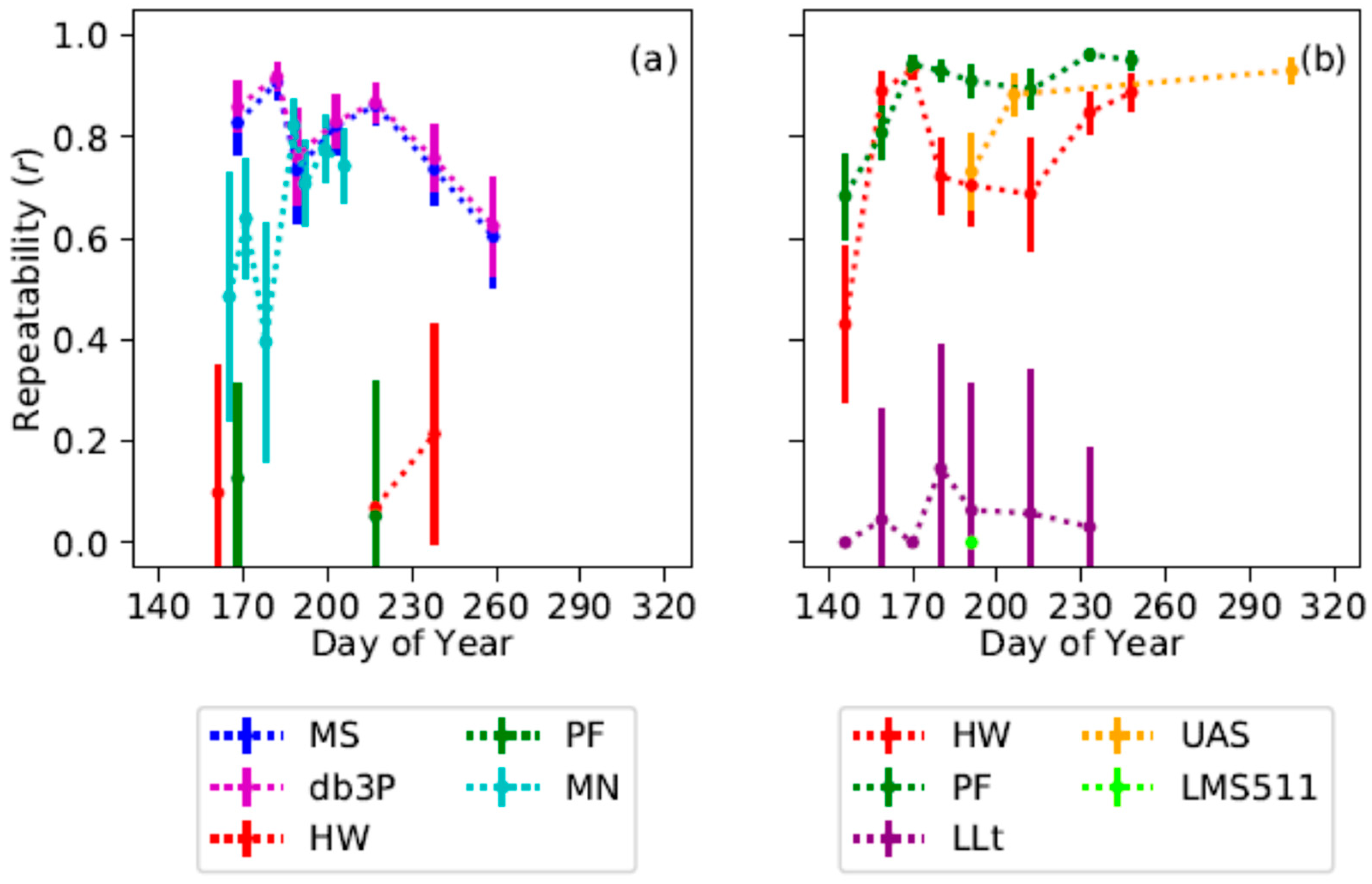
2.4.4. Sensor Performance and Plot-Level Statistical Analysis

In 2016, nadir view sensor precision and accuracy were evaluated against the manual plant height measurements. Since manual measurements were taken from the central zone of each row from each plot (mid-plot), the corresponding maximum height from each sensor was used for regression analysis (Figure 2b). As manual and tractor measurements were not conducted on the same days, measurements were paired to minimize the difference between collection dates and reduce error (Table 2). Based on the manual measurements, the cotton plants grew an average of 0.8 cm per day, so dates were paired such that four days (~3.2 cm) was the maximum difference. The r² values were calculated using a Python script with the “scipy.stats” and “numpy” packages and visualized with “pyplot”. In 2017, nadir and multi-angle view derived plot-level mean plant heights were evaluated against the Pepperl+Fuchs plot-level mean plant heights. As in 2016, not all measurements were conducted on the same days, so measurements were paired to minimize the difference between collection dates and reduce error. The r² values and visualization were performed using the Python script described above.

To identify and remove significant outliers from the plot-level means, a mixed linear model for each sensor and/or platform from each collection was fitted using ASReml-R version 3.0 [31]. The model used was the same as described above (Model 1). Outliers were identified using Studentized deleted residuals with degrees of freedom being calculated using the Kenward and Rogers approximation [32]. Once plot-level mean outliers were removed, an iterative mixed linear model fitting procedure was conducted in ASReml-R version 3.0 using Model 1 as above. To remove all non-significant random terms from the full model, likelihood ratio tests were conducted with a significance threshold set at α = 0.05 generating a final, best fitted model for each sensor and/or platform from each collection [33]. This final model was used to generate best linear unbiased estimators (BLUEs) for each cotton entry across the irrigation treatments within the respective year. Sequential tests of fixed effects were carried out with degrees of freedom being calculated with the Kenward and Rogers approximation in ASReml-R version 3.0.

For each sensor and/or platform, repeatability (r) was calculated to express the proportion of the variance due to permanent, non-localized differences between cotton entries providing a measure of technical performance (Model 2). Model 1 was reformulated so that all terms were modeled as random effects to estimate the respective variance components for use in Model 2. The variance component estimates for the full model were used to estimate r as follows:

$$r=\frac{\widehat{{\sigma }_{\alpha }^2}}{\widehat{{\sigma }_{\alpha }^2}+ \frac{\widehat{{\sigma }_{\alpha \beta }^2}}{\mathrm{n}\mathsf{\beta }}+ \frac{\widehat{{\sigma }_{\epsilon }^2}}{n\mathsf{\xi } }}$$

(2)

where $\widehat{{\sigma }_{\alpha }^2}$ was the estimated variance due to the cotton entry, $\widehat{{\sigma }_{\alpha \beta }^2}$ was the estimated variance associated with cotton entry by irrigation treatment, $\widehat{{\sigma }_{\epsilon }^2}$ was the residual error variance. The variable nβ was the harmonic mean of the number of irrigation treatments in which each cotton entry was observed, and nξ was the harmonic mean of the number of plots in which each cotton entry was observed. The denominator of Model 2 is the equivalent to the phenotypic variance, $\widehat{{\sigma }_p^2}$. Standard errors of the estimated repeatability were approximated using the delta method [34,35].

3. Results

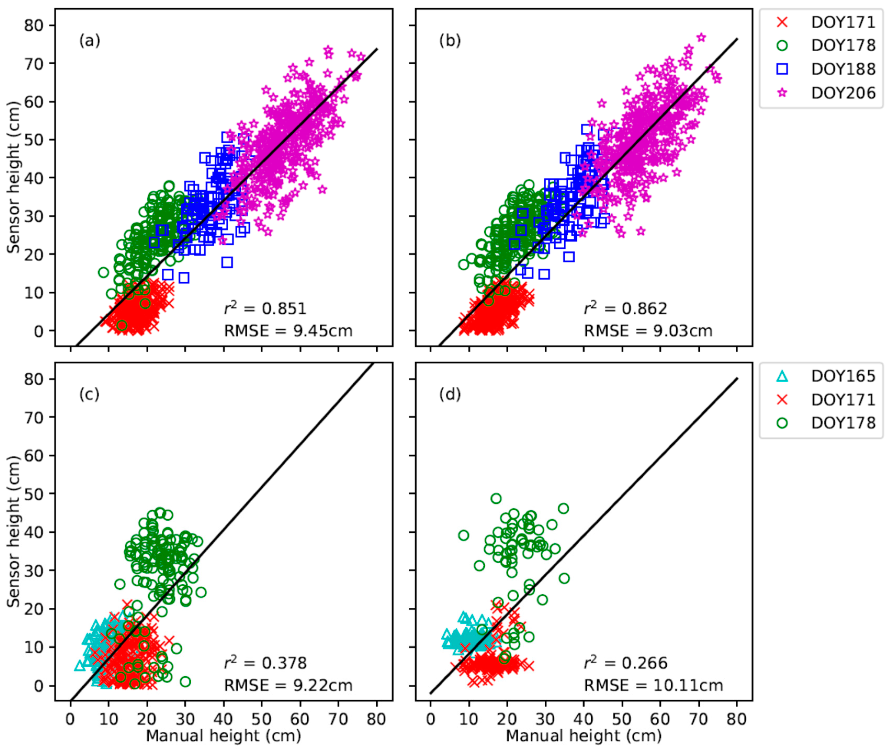
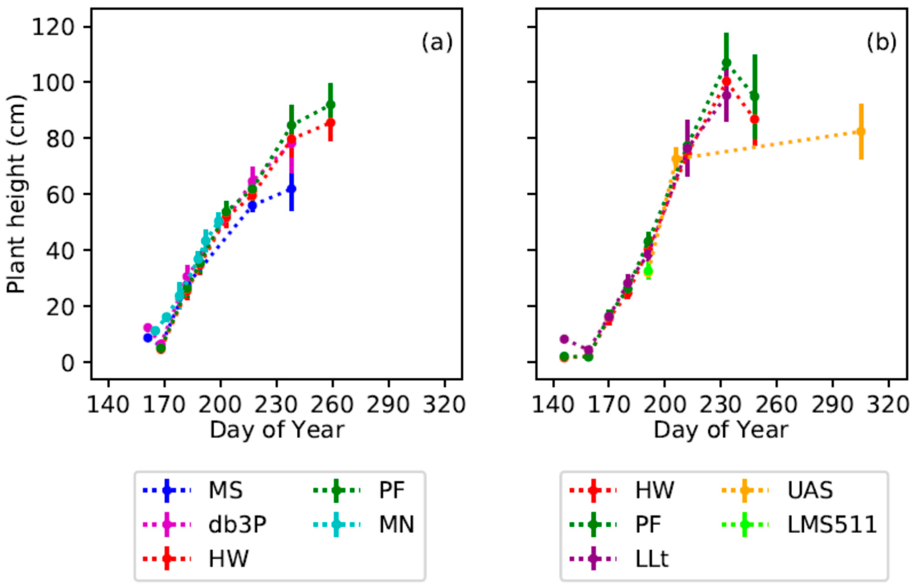
3.1. 2016 Estimates of Plant Height with Manual Measurements and Nadir View Sensors

Comparing plant heights obtained from the four nadir view ultrasonic transducers in 2016 with manual measurements revealed varying levels of agreement across the 360 mid-plot measurements. The Honeywell (HW) and Pepperl+Fuchs (PF) sensors (Figure 5a,b) showed strong correlations between the two sets of measurements (r² values 0.85 and 0.86, respectively) while the MaxSonar (MS) and db3 Pulsar (db3P) sensors (Figure 5c,d) showed weak correlations with the manual measurements (r² values 0.37 and 0.26, respectively). The root mean squared errors (RMSE) ranged from 9.03 to 10.11 cm. The RMSE was affected by the differences in collection days between the sensors and manual measurements causing increased error. All four sensors underestimated plant height when plants were small (DOY 165 and 171) which is attributed to soil interference or lower canopy leaves within the sensor field-of-view (FOV). On DOY 188 all sensors overestimated plant height, which is attributed to a mis-recording of the soil line to sensor boom height affecting the raw plant height calculations.

The standard deviation of plot-level plant height means recorded by each sensor increased over time for each variety grown (Figure 6a, Figure S1). Some increased deviation is expected with multiple varieties as each genotype will express the trait differently over time. The db3P sensor showed the greatest increase in deviation where the HW showed the least (Figure 5a, Table S1). The calculated repeatability (r) for the db3P sensor was consistently low (0.0–0.13) compared to the HW and PF sensors (Figure 7a, Table S2). This indicates more of the calculated deviation for the db3P was caused by the sensor rather than the expected genotype variation. The deviation in the manual measurements ranged from 1.19–4.59 cm (Figure 6a, Table S1) and the r increased as the season progressed (Figure 7a, Table S2). This could be attributed to the summer interns becoming more familiar with the barcode scanner equipment and demonstrates the effect human error can have on repeated manual measurements. The low deviation and high r of the HW and PF sensors indicate that temporal genotypic differences can effectively be measured by proximal UTs.

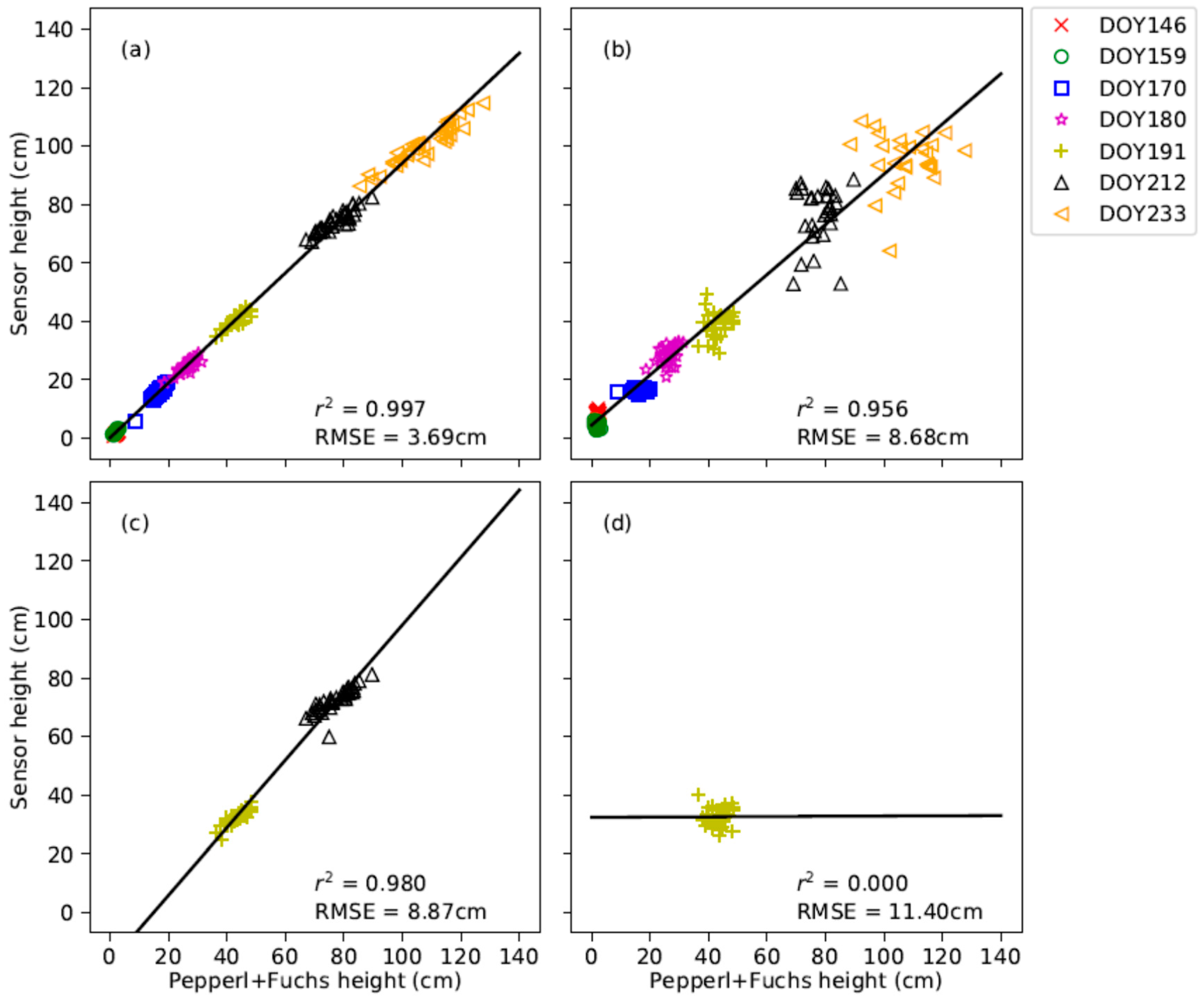
3.2. 2017 Estimates of Canopy Height with Nadir and Multi-Angle View Sensors

In 2017, the plot-level plant height means from the multi-angle view sensors, SICK-LMS511 (LMS511) and UAS derived images (UAS), and the nadir view LiDAR Lite v3 (LLt) were compared to the Pepperl+Fuchs (PF) ultrasonic transducers. The PF ultrasonics were used because of the stronger correlations and lower RMSE as compared with manual measurements in 2016 and higher repeatability. To determine across year consistency of the PFs, the Honeywell (HW) ultrasonics were retained in 2017 and compared with the PFs. A strong correlation (0.997) and a RMSE of 3.69 cm between the HW and PF sensors indicated consistency across years (Figure 8a). The RMSE for the multi-angle sensors (UAS and LMS511) and the nadir view LLt derived plant heights ranged from 8.68 to 11.40 cm. Of the two multi-angle view technologies, the UAS had the strongest correlation with the PF sensors at 0.980, which is higher than previously reported in sorghum (0.73 and 0.678) between UAS and manual measurements [16,22] (Figure 8c). The LMS511 was found to have no correlation with the PFs on the single day of collection and had the highest RMSE (11.40 cm), which is not consistent with previous findings in cotton where RMSE was estimated at 6.5 cm [20] (Figure 8d). This is due, in part, to “gaps” in the LiDAR scans as seen in the Figure 4c cross-section. These gaps are attributed tractor travel speed.

Similar to 2016, the standard deviation of the mean by each sensor increased over time (Figure 6b, Table S1). As seen in 2016 the HW sensors showed less deviation compared to the PFs during the season (Figure 6b, Table S1). The LLt showed similar deviation to the HW sensor (Figure 6b, Table S1) but had the greatest variation in estimated height over time (Figure S2c). The variation in heights are likely due to the very narrow beam angle of the sensor causing a small FOV. This reduced FOV means that instead of delineating the canopy profile, the beam penetrated the cotton canopy and returned distances from lower leaves or branches or detected profiles with reduced leaf angle (i.e., wilt) caused by the irrigation treatment at time of capture.

The HW, PF, and UAS had higher repeatability (r) ranging from 0.43 to 0.95 than the other sensors in 2017 (Figure 7b, Table S2). The HW r values were similar to findings from 2016, however the values decreased on DOYs 180, 191, and 206 (Figure 7b). These results may indicate that the HW sensor were more prone to thermal drift in this year or that the sensors need to be replaced. The PF sensor consistently had the highest r values both within and between years. The LLt consistently had low r throughout the season and reflects the increased variability seen in the growth curve (Figure 7b and Figure S2c). This indicates proximal nadir view lidar methods may not be the most effective for measuring plant height in the complex cotton canopy. These results highlight the importance of calculating FOV for nadir view fixed angle sensors to assess their suitability for measuring the desired trait.

4. Discussion

Of the four ultrasonic transducers (UT) tested in 2016, the Honeywell (HW) and Pepperl+Fuchs (PF) had the strongest correlations with manual measurements, low RMSE, low variability, and high repeatability. These two sensors had the smallest beam angles and calculated field-of-views (FOV) of the nadir view sensors aside from the LidarLite v3 (LLt). The smaller beam angles, along with the proximal position to the plants detected less variance in the canopy enabling a more accurate delineation of the canopy profile from which height was estimated. The wider beam angle and calculated FOV of the db3 Pulsar (db3P) and MaxSonar (MS) indicates the sensors also detected lower canopy leaves leading to increased variation in the collected data as these lower leaves “contaminated” the readings. Mounting the db3P and MS sensors lower, relative to the canopy profile, may improve the precision of these sensors thereby decreasing variability and increasing the repeatability of the measurements. This is supported in previous findings by Andrade-Sanchez et al. [14] where the db3P was mounted 0.3 m above the canopy and RMSE ranged from 4 cm to 7 cm with manual measurements. Transducer placement in the vertical plane (z-offset) should be determined by considering how the beam angle and sensor FOV relate to the width of the intended plant target. Better estimates of plant height can be obtained when the UT sensor views only the uppermost leaves and lower canopy leaves are excluded from view. Comparison of the HW and PF showed the PFs to have slightly higher repeatability values (r) in 2016 and maintained higher r values in 2017 indicating it is the more effective UT sensor for cotton height measurements.

The Lidar Lite v3 (LLt) gave the most accurate plant height measurements of the two LiDAR systems tested. Despite strong correlations with the PF measurements, the calculated repeatability for this sensor was consistently low, and variation in the captured data was high. This is likely due to the much narrower beam angle, approximately 1/8 that of the HW and PF sensors, which would consistently penetrate the canopy structure, missing the upper canopy leaves that are within the FOV of the ultrasonic sensors. These results were similar to those reported by Wang et al. [16] in young sorghum plants, where poor emergence showed peaks and valleys in the Lidar Lite v2 data plot profile that was smoothed out in the ultrasonic sensor profile. Given this variation, the LLt was determined to be less effective for determining cotton plant height but could be valuable in detecting other architectural or drought related traits. Further testing is needed for this sensor to determine if it will be useful for other architectural traits.

The LMS511 did not perform as expected based on previous reports by Madec et al. [19] or Sun et al. [20] who found proximal multi-angle LiDAR measurements to be an effective means of estimating plant height in cotton and wheat, respectively. There are several reasons why the LMS511 data presented in this study do not compare to those previously reported including differences in planting density, tractor speed, and mounting position. The tractor speed in this study was double the speed reported in other studies [19,20]. The faster speeds reduced the total number of scans per plot and left “gaps” in the plot profile. The reduction in data prevented identification of heights from each plot zone, skewing the plot average. A final factor to consider was the placement of the LMS511 in this study relative to that in Madec et al. [19] and Sun et al. [20]. In this study, the LMS511 was mounted in between the plot rows to capture a whole plot (i.e., two rows) in one pass. Madec et al. [19] and Sun et al. [20] mounted their LiDAR instruments directly over the plot row ensuring the tops of all plants would be captured. Mounting the LiDAR over the inter-row area diminished the ability to capture a full vertical profile of the plant, leading to underestimated plant height in some of the taller varieties. The tractor speed, sensor placement, row spacing, and collection time-of-day presented in this paper follow previous collection methods described by Pauli et al. [5], Andrade-Sanchez et al. [14], and Thompson et al. [15] for capture of heat and drought-related traits, which are the primary focus of the research occurring at this location. The results of this study suggest the LMS511 is not compatible with the previous collection methods and requires a separate platform and collection protocol to be effective. In addition, the intensive computational requirements for LiDAR data and the cost, reduces the efficiency of LiDAR for characterizing plant height in the cotton breeding program but could be valuable in detecting very detailed traits of the canopy architecture.

The UAS image-based 3-D point clouds performed the best overall for the two multi-angle view technologies tested. The correlation with the PF ultrasonics was similar to previous findings in wheat [19] but stronger than those reported in sorghum [16,22]. The sorghum studies utilized a similar approach to estimate plant height from the UAS image-based 3-D point clouds where the drone altitude during flight was used to calculate the z-axis value (soil line reference) across the entire field. Previous experience has shown that UAS altitude is not constant during overflight even though it is reported as such in the image EXIF information. Herein, a strategy was devised for referencing plant measurements to local bed measurements in the 3-D point cloud. The z-axis reference was calculated for each plot zone using four known localized bare soil reference areas per plot (two per row). A similar strategy of referencing plot data to localized bare soil data was also performed in the Madec et al. [19] study, although the methodology was different. The repeatability estimates estimated from the UAS-generated data in this study were high and increased with each collection. The change in flight altitude, which decreased with each successive flight, improved the spatial resolution of the 3-D point cloud. Future UAS flights that intend to estimate plant height should fly 15 to 30 m above the canopy and ensure sufficient alley row spacing for referencing experimental plot data to localized bare soil reference data in the alleyway area. Future data processing should also include an outlier removal step prior to calculating the final plot average, which was not done in this study. Removal of outliers would improve overall estimates of plant height by reducing variation in the data.

The results presented in this study describe the efficiency and effectiveness of different sensors for estimating plant height in cotton. The ultrasonic transducers were the easiest to deploy and had relatively simple data processing requirements. They also provided accurate estimates of plant height which were repeatable across the growing season and separate years. The only drawback with the UTs in this study was the overestimation of plant height when plants were small due to bed (soil) interference in the sensor FOV. In the future, a bed height interpolation similar to the UAS data processing could reduce the error seen with small plants. The 3-D point clouds derived from the UAS were also very effective for estimating plant height, although the computational requirements for processing the data were higher than those for ultrasonics. Also, specialized expertise and certification is legally required to deploy the UAS for research purposes. Of the two proximal LiDAR systems tested, the LidarLite v3 was more efficient and effective than the SICK despite its lower cost. Although the LiDAR Lite v3 did well and had similar efficiency in terms of deployment and data processing, it was considered less effective than the ultrasonics. However, this sensor may perform better in less complex plant architectures than cotton. The LMS511 had the least efficiency and effectiveness overall which was due to the capture method. Future studies are needed to determine the best platform and deployment protocol for this sensor; however, the cost, effort required for data capture and processing will likely still make it inefficient to characterize plant height for breeding programs with limited resources and expertise. The instrument may be most useful for characterizing discrete distance in more complex plant architectural traits like leaf angle, canopy volume, and fruit load.

5. Conclusions

Plant height is an important phenotype for cotton management and an indicator of plant health. This study shows that simple and relatively inexpensive industrial ultrasonic transducers are an effective and efficient means of measuring cotton plant height over time. Three-dimensional point clouds generated by photogrammetry from UAS-based images were also found to be an effective way to measure plant height. The LiDAR sensors explored in this study were found to be less effective and efficient overall but may have more intrinsic value for more complex traits such as leaf and branching angle.

References

1. Food and Agriculture Organization of the United States. FAOSTAT: Production/Crops. 2016. Available online: http://www.fao.org/faostat/en/#data/QC/visualize (accessed on 19 October 2018).
2. Cotton Incorporated. Monthly Economic Letter: Cotton Market Fundamentals and Price Outlook. 2016. Available online: http://www.cottoninc.com/corporate/Market-Data/MonthlyEconomicLetter (accessed on 19 October 2018).
3. National Cotton Council of America. World of Cotton. 2018. Available online: http://www.cotton.org/econ/world/ (accessed on 19 October 2018).
4. Paterson, A.H.; Saranga, Y.; Menz, M.; Jiang, C.-X.; Wright, R.J. QTL analysis of genotype x environment interactions affecting fiber quality. Theor. Appl. Genet. 2003, 106, 384–396. [Google Scholar] [CrossRef] [PubMed]
5. Pauli, D.; Andrade-Sanchez, P.; Carmo-Silva, A.E.; Gazave, E.; French, A.N.; Heun, J.; Hunsaker, D.J.; Lipka, A.E.; Setter, T.L.; Strand, R.J.; et al. Field-based high-throughput plant phenotyping reveals the temporal patterns of quantitative trait loci associated with stress-responsive traits in cotton. Genes Genomes Genet. 2016, 6, 865–879. [Google Scholar] [CrossRef] [PubMed]
6. Ware, J.O. Plant Breeding and the Cotton Industry; USDA Yearbook of Agriculture, U.S. Gov. Print Office: Washington, DC, USA, 1937; pp. 657–744.
7. Oosterhuis, D.M. Growth and Development of a Cotton Plant; Miley, W.N., Oosterhuis, D.M., Eds.; Nitrogen Nutrition of Cotton: Madison, WI, USA, 1990; pp. 1–24. [Google Scholar]
8. Hake, K.; Burch, B.; Mauney, J. Making sense out of stalks: What controls plant height and how it affects yield. In Physiology Today Newsletter; National Cotton Council: Memphis, TN, USA, 1989; p. 4. [Google Scholar]
9. Quisenberry, J.E.; Roark, B. Influence of indeterminate growth habit on yield and irrigation water-use efficiency in upland cotton. Crop Sci. 1976, 16, 762–765. [Google Scholar] [CrossRef]
10. Sui, R.; Fisher, D.K.; Reddy, K.N. Cotton yield assessment using plant height mapping system. J. Agric. Sci. 2013, 5, 23–31. [Google Scholar] [CrossRef]
11. White, J.W.; Andrade-Sanchez, P.; Gore, M.A.; Bronson, K.F.; Coffelt, T.A.; Conley, M.M.; Feldmann, K.A.; French, A.N.; Heun, J.T.; Hunsaker, D.J.; et al. Field-based phenomics for plant genetics research. Field Crops Res. 2012, 133, 101–112. [Google Scholar] [CrossRef]
12. Deery, D.; Jimenez-Berni, J.; Jones, H.; Sirault, X.; Furbank, R. Proximal remote sensing buggies and potential applications for field-based phenotyping. Agron. J. 2014, 5, 349–379. [Google Scholar] [CrossRef]
13. Lin, Y. LiDAR: An important tool for next-generation phenotyping technology of high potential for plant phenomics? Comput. Electron. Agric. 2015, 199, 61–73. [Google Scholar] [CrossRef]
14. Andrade-Sanchez, P.; Gore, M.A.; Heun, J.T.; Thorp, K.R.; Carmo-Silva, A.E.; French, A.N.; Salvucci, M.E.; White, J.W. Development and evaluation of a field-based high-throughput phenotyping platform. Funct. Plant Biol. 2014, 41, 68–79. [Google Scholar] [CrossRef] [Green Version]
15. Thompson, A.L.; Thorp, K.R.; Conley, M.; Andrade-Sanchez, P.; Heun, J.T.; Dyer, J.M.; White, J.W. Deploying a proximal sensing cart to identify drought-adaptive traits in upland cotton for high-throughput phenotyping. Front. Plant Sci. 2018, 9, 507. [Google Scholar] [CrossRef] [PubMed]
16. Wang, X.; Singh, D.; Marla, S.; Morris, G.; Poland, J. Field-based high-throughput phenotyping of plant height in sorghum using different sensing technologies. Plant Methods 2018, 14, 53. [Google Scholar] [CrossRef] [PubMed]
17. Sirault, X.; Fripp, J.; Paproki, A.; Kuffner, P.; Nguyen, C.; LI, R.; Daily, H.; Gui, J.; Furbank, R. PlantScan: A three-dimensional phenotyping platform for capturing the structural dynamic of plant development and growth. In Proceedings of the International Conference on Functional-Structural Plant Models, Helsinki, Finland, 12–13 December 2013. [Google Scholar]
18. French, A.N.; Gore, M.A.; Thompson, A.L. Cotton phenotyping with LIDAR from a track-mounted platform. In Proceedings of the Autonomous Air and Ground Sensing Systems for Agricultural Optimization and Phenotyping, Baltimore, MD, USA, 17–21 April 2016. [Google Scholar]
19. Madec, S.; Baret, F.; De Solan, B.; Thomas, S.; Dutartre, D.; Jezequel, S.; Hemmerlé, M.; Colombeau, G.; Comar, A. High-throughput phenotyping of plant height: Comparing unmanned aerial vehicles and ground LiDAR estimates. Front. Plant Sci. 2017, 8, 2002. [Google Scholar] [CrossRef] [PubMed]
20. Sun, S.; Changying, L.; Paterson, A.H. In-field high-throughput phenotyping of cotton plant height using LiDAR. Remote Sens. 2017, 9, 337. [Google Scholar] [CrossRef]
21. Busemeyer, L.; Mentrup, D.; Möller, K.; Wunder, E.; Alheit, K.; Hahn, V.; Maurer, H.; Reif, J.; Würschum, T.; Müller, J.; et al. BreedVision—A multi-sensor platform for non-destructive field-based phenotyping in plant breeding. Sensors 2013, 13, 2830–2847. [Google Scholar] [CrossRef] [PubMed]
22. Watanabe, K.; Guo, W.; Arai, K.; Takanashi, H.; Kajiya-Kanegae, H.; Kobayashi, M.; Yano, K.; Tokunaga, T.; Fujiwara, T.; Tsutsumi, N.; et al. High-throughput phenotyping of sorghum plant height using an unmanned aerial vehicle and its application to genomic prediction modeling. Front. Plant Sci. 2017, 8, 421. [Google Scholar] [CrossRef] [PubMed]
23. Troscianko, J.; Stevens, M. Image calibration and analysis toolbox—A free software suite for objectively measuring reflectance, colour and pattern. Methods Ecol. Evol. 2015, 6, 1320–1331. [Google Scholar] [CrossRef] [PubMed]
24. Allen, R.G.; Pereira, L.S.; Raes, D.; Smith, M. Crop Evapotranspiration—Guide-Lines for Computing Crop Water Requirements; FAO Irrigation and Drainage Paper 56; Food and Agriculture Organization of the United Nations: Rome, Italy, 1998. [Google Scholar]
25. Hunsaker, D.J.; Barnes, E.M.; Clarke, T.R.; Fitzgerald, G.J.; Pinter, P.J. Cotton irrigation scheduling using remotely sensed and FAO-56 basal crop coefficients. Trans. ASABE 2005, 48, 1395–1407. [Google Scholar] [CrossRef]
26. Brown, P.W. Accessing the Arizona Meteorological Network (AZMET) by Computer; Extension Report No. 8733; University of Arizona: Tucson, AZ, USA, 1989. [Google Scholar]
27. Wang, X.; Thorp, K.R.; White, J.W.; French, A.N.; Poland, J.A. Approaches for geospatial processing of field-based high-throughput plant phenomics data from ground vehicle platforms. Trans. ASABE 2016, 59, 1053–1067. [Google Scholar]
28. Kutner, M.H.; Nachtsheim, C.J.; Neter, J.; Li, W. Applied Linear Statistical Models; McGraw-Hill Irwin: New York, NY, USA, 2004. [Google Scholar]
29. Shen, S. Accurate multiple view 3D reconstruction using patch-based stereo for large-scale scenes. IEEE Trans. Image Process. 2013, 22, 1901–1914. [Google Scholar] [CrossRef] [PubMed]
30. Point Cloud Library. The PCD (Point Cloud Data) File Format. 2018. Available online: http://pointclouds.org/documentation/tutorials/pcd_file_format.php#pcd-file-format (accessed on 5 November 2018).
31. Gilmour, A.R.; Gogel, B.J.; Cullis, B.R.; Thompson, R. ASReml User Guide Release 3.0; VSN International Ltd.: Hemel Hempstead, UK, 2009. [Google Scholar]
32. Kenward, M.G.; Roger, J.H. Small sample inference for fixed effects from restricted maximum likelihood. Biometrics 1997, 53, 983–997. [Google Scholar] [CrossRef] [PubMed]
33. Littell, R.C.; Milliken, G.A.; Stroup, W.W.; Wolfinger, R.D.; Schabenberger, O. SAS for Mixed Models; SAS Institute: Cary, NC, USA, 2006. [Google Scholar]
34. Lynch, M.; Walsh, B. Genetics and Analysis of Quantative Traits; Sinauer Associates, Inc.: Sunderland, MA, USA, 1998. [Google Scholar]
35. Holland, J.B.; Nyquist, W.E.; Cervantes-Martinez, C.T. Estimating and Interpreting Heritability for Plant Breeding: An Update; Janick, J., Ed.; Plant Breeding Reviews Wiley: Hoboken, NJ, USA, 2003. [Google Scholar]
Figure 1. The high-clearance Lee Agra Avenger tractor fitted with a modified front boom using aluminum T-slot to mount the proximal sensors. The four arms on the modified boom that carry the sensors which include inertial measurement unit (IMU), real-time kinematic—global positioning system (RTK-GPS) and two ultrasonic transducer sensors (MaxSonar and dB3) in 2016 (a), and the sensor array used in 2017 data collections (b).
Remotesensing 11 00700 g001
Figure 2. Field experimental layout (a) for a cotton study comparing regional breeders testing network germplasm with two irrigation rates in 2016 and 2017 growing seasons at Maricopa, Arizona, USA. The two-row, 12.1 m plots are outlined in black, the 48-plot zones are outlined in grey, the mid-plot for manual measurements are outlined in red, and the 0.5 m diameter soil bed polygons are colored green (b) shown with an RGB composite image of the field on 10 July 2017.
Remotesensing 11 00700 g002
Figure 3. Flow chart for nadir view sensors (ultrasonic transducers and Lidar Lite V3) data processing with an example output of raw plant heights georeferenced by the UTM coordinates from the 2017 DOY191 Pepperl+Fuchs sensors.
Remotesensing 11 00700 g003
Figure 4. Flow chart for multi-angle view sensors (UAS and LMS511) data processing. The green boxes and arrows depict steps unique to the UAS and blue, steps unique to the LMS511 (a). Example outputs (3-D cloud and 2-D cross section) of raw plant heights georeferenced by the UTM coordinates from the 2017 DOY191 UAS collection (b) and plants heights before bed height interpolation from the 2017 DOY191 LMS511 collection (c).
Remotesensing 11 00700 g004aRemotesensing 11 00700 g004b
Figure 5. Manual plant height measurements (cm) compared to the Honeywell (HW) (a); Pepperl+Fuchs (PF) (b); MaxSonars (MS) (c); and db3 Pulsar (db3P) (d) height measurements within the 360 mid-plots grown at that Maricopa Agricultural Center in Maricopa, AZ in 2016 on the corresponding day of year (DOY).
Remotesensing 11 00700 g005
Figure 6. Calculated plant height (cm) means and standard deviation obtained from the Honeywell (HW), Pepperl+Fuchs (PF), MaxSonar (MS), db3 Pulsar (db3P), and manual measurements (MN) across the growing season in 2016 (a), and the means and standard deviations for the Honeywell (HW), Pepperl+Fuchs (PF), LidarLite v3 (LLt), unmanned aerial system images (UAS), and SICK-LMS511 (LMS511) sensors used to collect plant height data across the 2017 growing season (b).
Remotesensing 11 00700 g006
Figure 7. Estimated repeatability (r) for plant height measured using the Honeywell (HW), Pepperl+Fuchs (PF), MaxSonar (MS), db3 Pulsar (db3P), and manual measurements (MN) in 2016 (a); and the Honeywell (HW), Pepperl+Fuchs (PF), LidarLite v3 (LLt), unmanned aerial system images (UAS), and SICK-LMS511 (LMS511) sensors in 2017 (b) for each collection day.
Remotesensing 11 00700 g007
Figure 8. Pepperl+Fuchs (PF) derived plant height (cm) plot-level means compared to the Honeywell (HW) (a); LiDAR Lite v3 (LLt) (b); unmanned aerial system (UAS) (c); and LMS511 (d) height measurements for all 35 cotton entries grown at that Maricopa Agricultural Center in Maricopa, AZ in 2017.
Remotesensing 11 00700 g008