Quantifying the Effects of Urban Form on Land Surface Temperature in Subtropical High-Density Urban Areas Using Machine Learning

1
Geography & Spatial Information Techniques Department, Ningbo University, Ningbo 315211, China
2
School of Resources and Environment, Hubei University, Wuhan 430062, China
3
Zhejiang Academy of Social Science, Hangzhou 310007, China
*
Author to whom correspondence should be addressed.
Remote Sens. 2019, 11(8), 959; https://doi.org/10.3390/rs11080959
Submission received: 28 January 2019
/
Revised: 16 April 2019
/
Accepted: 18 April 2019
/
Published: 22 April 2019
(This article belongs to the Special Issue Remote Sensing Based Fine-Scale Urban Thermal Environment)
Abstract
:It is widely acknowledged that urban form significantly affects urban thermal environment, which is a key element to adapt and mitigate extreme high temperature weather in high-density urban areas. However, few studies have discussed the impact of physical urban form features on the land surface temperature (LST) from a perspective of comprehensive urban spatial structures. This study used the ordinary least-squares regression (OLS) and random forest regression (RF) to distinguish the relative contributions of urban form metrics on LST at three observation scales. Results of this study indicate that more than 90% of the LST variations were explained by selected urban form metrics using RF. Effects of the magnitude and direction of urban form metrics on LST varied with the changes of seasons and observation scales. Overall, building morphology and urban ecological infrastructure had dominant effects on LST variations in high-density urban centers. Urban green space and water bodies demonstrated stronger cooling effects, especially in summer. Building density (BD) exhibited significant positive effects on LST, whereas the floor area ratio (FAR) showed a negative influence on LST. The results can be applied to investigate and implement urban thermal environment mitigation planning for city managers and planners.

1. Introduction
An urban heat island (UHI) has been observed and recognized to exist in the most of cities around the world [1]. Compared to their surrounding rural areas, an elevated temperature of urban areas not only directly affects urban ecological environment quality, but also increases human risk of violence and mortality, thus impacting on mental well-being of urban residents and overall livability of cities [2,3,4,5,6,7]. The elderly and children can be more easily influenced by higher outdoor air temperature. Suicide rates may rise 0.7 percent in the United States and 2.1 percent in Mexico for a 1 °C increase in monthly average temperature [8]. As a result, although UHI was first discovered about two centuries ago, it is still an important research topic across various fields of study [9]. How to alleviate the UHI effect is an issue of considerable interest [10]. The urban form influences and is influenced by the flows of people, energy, and matter [11], and it is widely believed that physical urban form significantly affects urban thermal environments [12,13,14,15]. Accordingly, an understanding of the complex relationships between features of urban form and the land surface temperature (LST) is critically important to mitigate the UHI and provide guidance for the environmentally-friendly planning of cities.
Urban form refers to the spatial structure and form of urban elements, including land use, transport infrastructure, water and energy infrastructure, and the physical form of developments that facilitate human activities and their interactions [14,15,16]. Urban form is a key element for understanding urban systems as social–economic–natural hybrids. Previous research has demonstrated the relationships between urban surface characteristics such as land use composition, landscape configuration, remote sensing ecology index, building features parameters, and LST. Generally, land use composition influences LST directly by affecting the physical characteristics of the surface, such as moisture and albedo [2]. Urban artificial landscape composition, such as building and open soil, tends to amplify the UHI effects, while natural landscape compositions (e.g., farmland, forests, grassland, water bodies, and wetlands) have cooling effects on urban thermal environments [17,18,19]. Most researches have indicated that the normalized difference vegetation index (NDVI) has a strong negative correlation with LST, while the normalized difference built-up index (NDBI) and the impervious surfaces fraction (ISA) both show an obvious positive correlation with LST [20]. In the context of rapid and extensive urbanization, The LST values exhibited an associated overall increase along with land use and land cover (LULC) change in some fast-growing cities [21], and the LULC–UHI relationship is always non-linear [22]. Future urban temperatures and heat stress will be amplified in both rural and urban areas [23].
For high-density urban areas, more and more researches examined the potential relationships between building features in 2D/3D and LST. Guo et al. [24] and Giridharan et al. [25] have argued that the LST tends to be much cooler where there is low building density and high floor area ratio (FAR). Yin et al. [14] found that both higher sky view factor (SVF) and building density intensified the UHI effect, while FAR had the opposite effect on LST. Dense building blocks were accompanied by a high-density population and less shading or ventilation, and produced more waste heat to release into the outdoor atmosphere environment, thus creating severe UHI effects. In a densely built section of the City of Columbus, researchers also concluded that increasing building roof-top areas and solar radiations lead to increased LST, while increasing NDVI, SVF, and water lead to decreasing LST [26]. Chun et al. [27] further examined the seasonality of the impacts of building rooftop and façade areas, urban canyons, water bodies, vegetation, and solar radiation, on UHI intensity. They found that building footprints had stronger positive effects on the UHI during the warmer months, and building wall areas have no significant effects in winter, as well as in June. Urban architectural patterns (e.g., frontal area density) were also one of the important drivers of local urban surface temperature. High-density high-rise buildings can increase surface temperatures in the city center [28,29].
A thorough examination of the literature reveals the relevancies of urban form and LST varies with the heterogeneity of urban background in the socio-economic, climate zone, and eco-environment. On the other hand, Wentz et al. [11] identified and defined six fundamental aspects of urban form: (1) Human constructed elements, (2) the soil-plant continuum, (3) water elements, (4) two- and three-dimensional space, (5) spatial pattern of urban areas, and (6) time. As far as we know, comprehensive and conclusive evidence regarding the influences of urban form on the LST is still lacking. The quantitative relationships between underlying variables of urban form features and LST should be examined on the multiple scales. This may be valuable for guiding urban thermal mitigation planning and constructing sustainable and comfortable urban systems.
Here, the objectives of this paper are to: (1) Determine the extent to which urban form metrics influence the LST variations considering the differences of seasonality and observation scales; (2) compare and estimate the modelling ability of two regression methods: Ordinary least-squares regression (OLS) and random forest regression (RF); and (3) assess the most suitable scale which can be used to capture the best explanatory and predictive power. Three observation scale grids, with cell sizes of 100 m, 200 m, and 400 m, were used to prepare all the data. Meanwhile, both two-dimensional and three-dimensional explanatory variables were used to represent the complex urban form features in high-density urban centers. The study will provide deeper insights for urban planners and managers on how to alleviate the UHI effect and improve the urban thermal environment by optimizing the local urban form.
2. Materials and Methods
2.1. Study Area
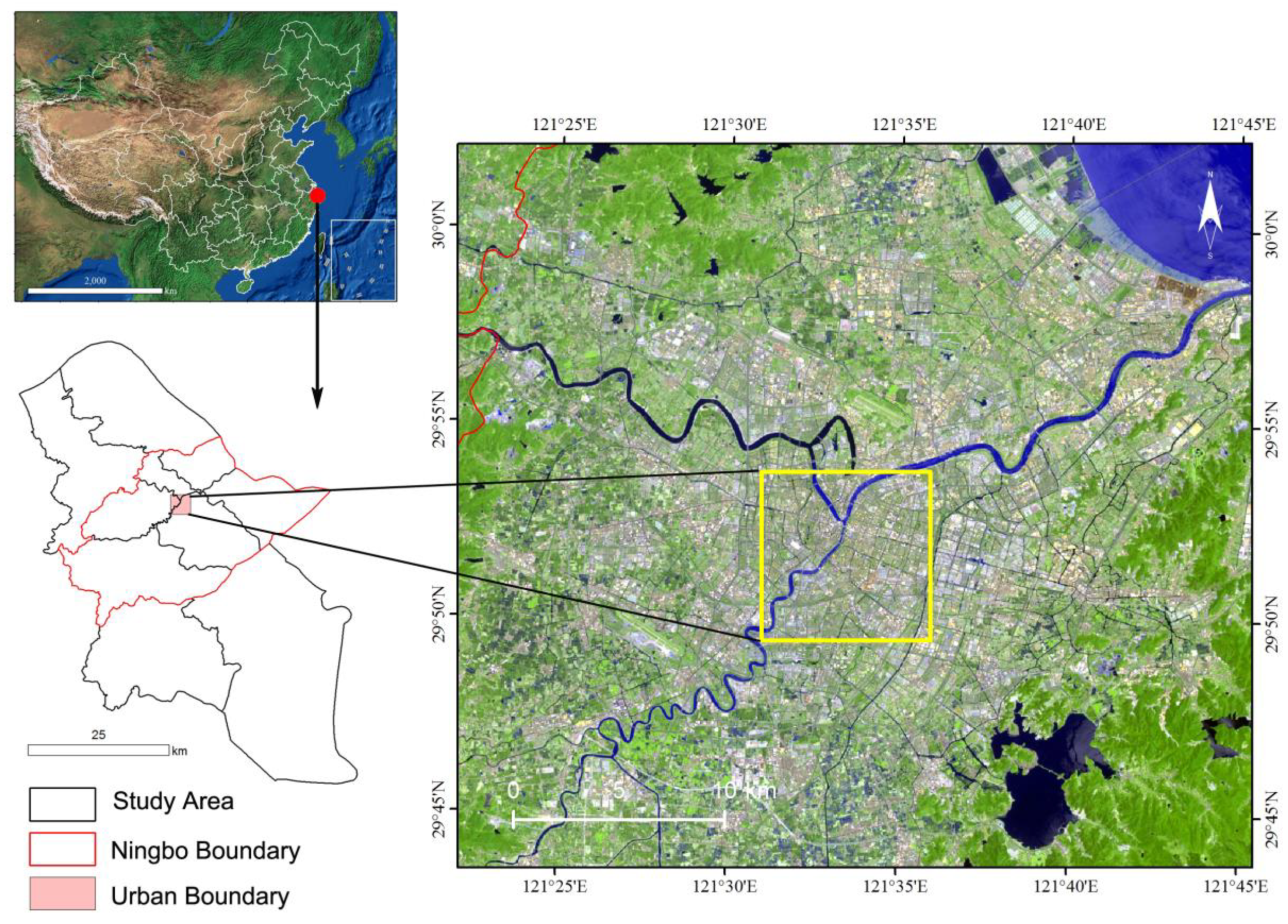
Ningbo is located in the south-east of Yangtze River Delta by the East China Sea (Figgure 1). Three major rivers flow through the plains of Ningbo: The Yao River, the Fenghua River, and the Yong River. The city has enjoyed the special designation of a ‘separate planning city’ since 1988, which grants it provincial level administrative status [30]. As a typical port city, Ningbo has become an important industrial and economic center in Zhejiang Province, China. However, the rapid development and urbanization of the last 40 years have created potential problems for the environment. Current climate change has also significantly increased the risk of extreme events. During 1984–2010, average UHI intensity was 8.67 °C in summer, and this effect tended to increase in summer [31]. In this study, we focus on the urban center of Ningbo with an area of 8 km × 8 km ≈ 64 km2 (see Figure 1b), namely the three estuaries. The region is the Central Business District (CBD) of the city, and aggregates numerous commercial, residential, office, and governmental units with high-density building.
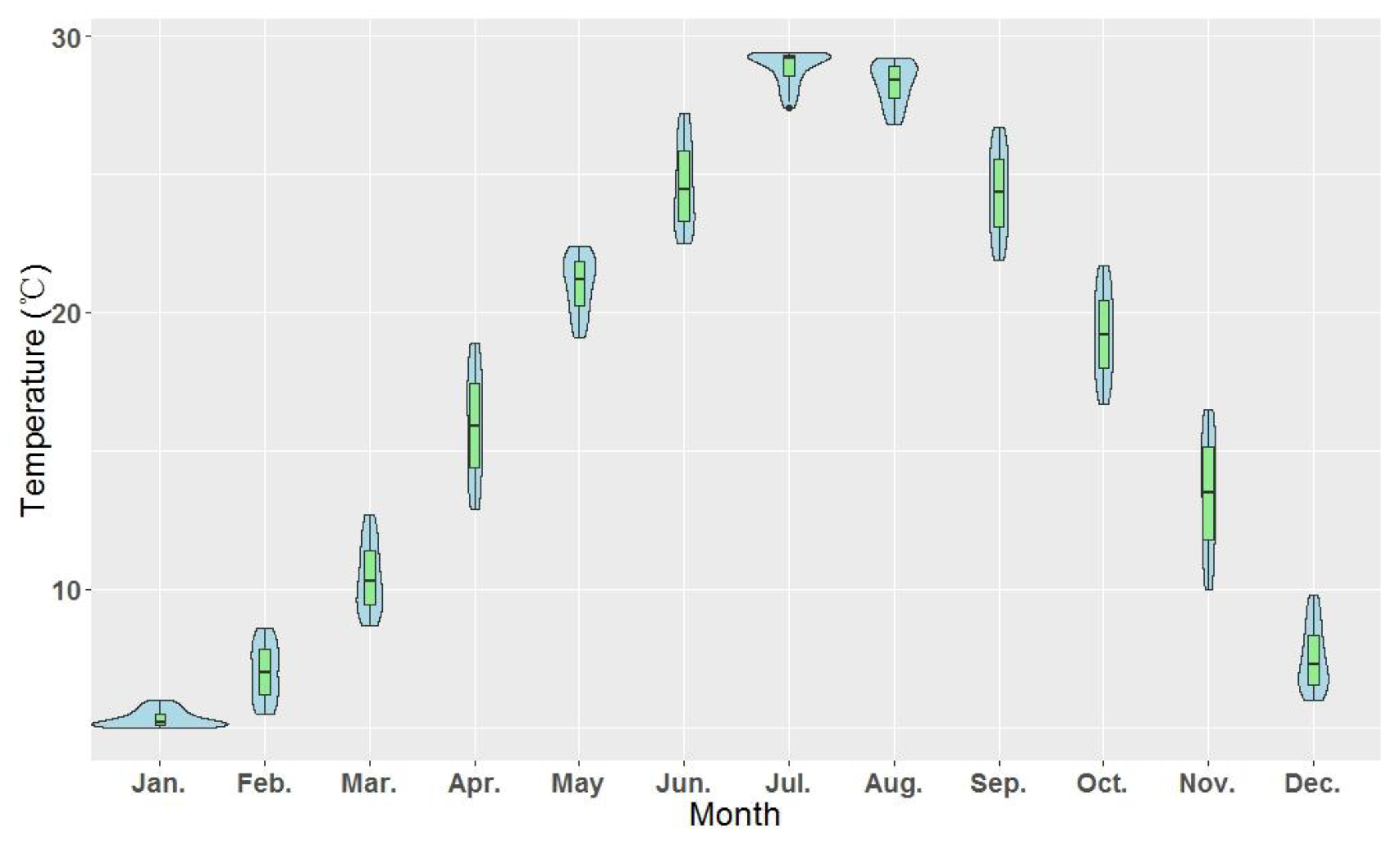
Ningbo has a humid subtropical climate with distinctive seasons, characterized by hot, humid summers and chilly, cloudy, and drier winters. As shown in Figure 2, the mean annual temperature was 17.22 °C during the past three decades, with the monthly daily averages ranging from 5.31 °C in January to 28.28 °C in August. Thus, July and August were the hottest months for one year with an average temperature exceeding 27 °C, while January and February were the coldest months in one year.
2.2. Urban Form
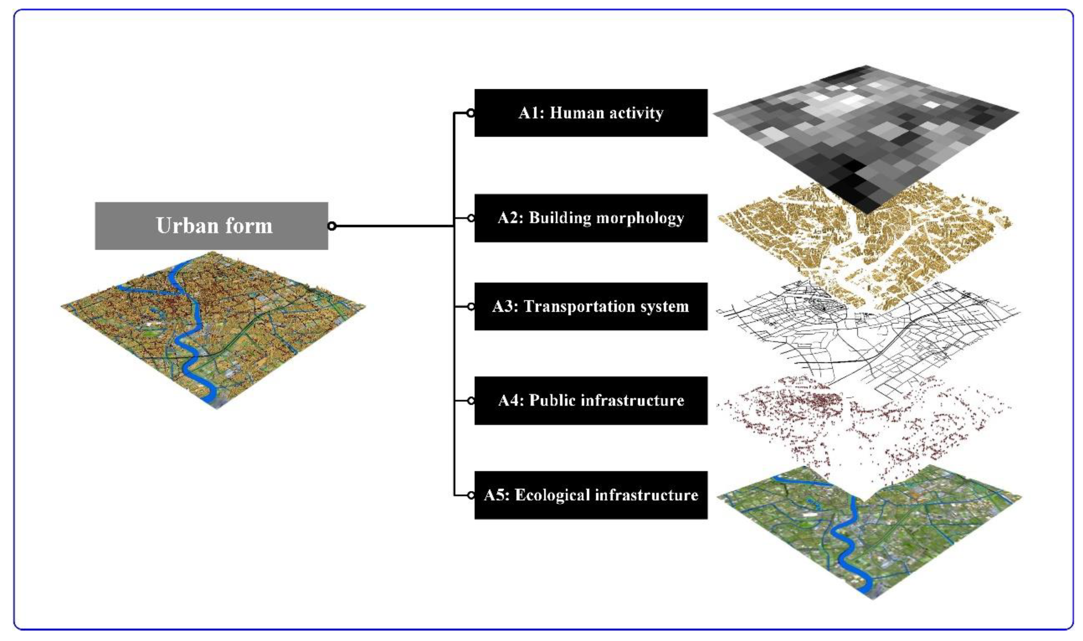
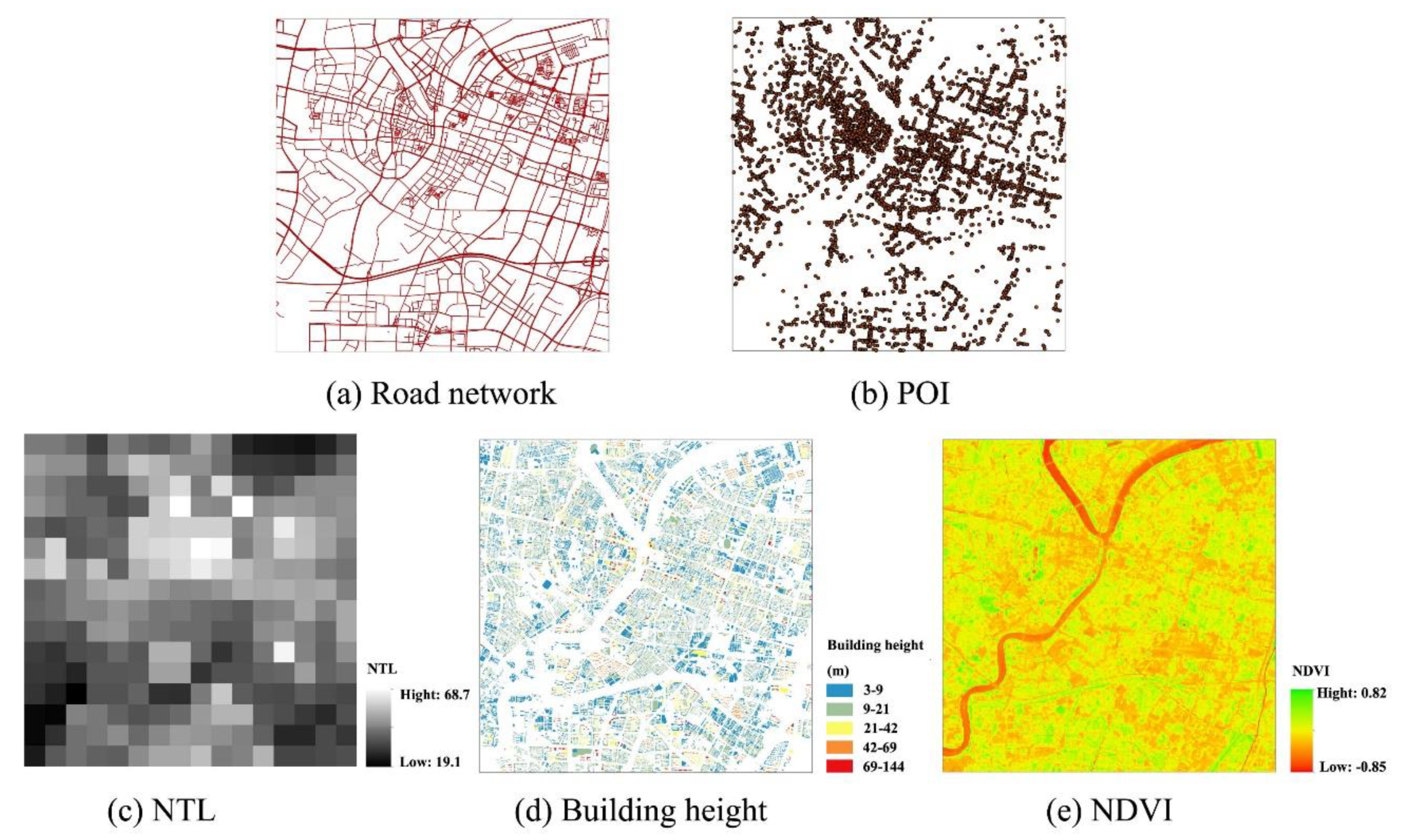
In this study, we redefine and disassemble the urban form into five aspects as shown in Figure 3: (A1) Human activity, which relates to the spatial distribution and behaviors of populations; (A2) building morphology, high-density buildings are the important human constructed materials in urban environments, and they are the primary component of urban form; (A3) transportation system, which consists of different levels of road network; (A4) public infrastructure, which represents the units providing public services, including hospitals, government agencies, schools, banks etc..; (A5) ecological infrastructure, refers to the urban public open space covered with green and water. With the help of remote sensing and spatial analysis technologies, most of the urban form metrics could be extracted and presented with two-dimensional and three-dimensional data. Within our proposed urban form analysis framework, seven representative LST model variables were selected in this paper as follows: (1) Human activity: nighttime light (NTL) intensity; (2) building morphology: Building density and floor area ratio; (3) transportation system: Road density; (4) public infrastructure: point of interest (POI) density; (5) ecological infrastructure: Water surface ratio, and NDVI.
- NTL intensity (NTLI): The NTLI is a reliable proxy for estimating and monitoring socioeconomic dynamics and human activities intensity. Herein, we used the composite NPP-VIIRS nighttime light data of the year 2015, which were obtained from the website of NOAA/NGDC (https://ngdc.noaa.gov/eog/viirs/download_dnb_composites.html).
- Building density (BD): The BD is the total area of building footprints within the regular observation grids. It is an important controlling index in urban planning and land management. Higher building density means higher intensity of land use and development.
- Floor area ratio (FAR): The FAR refers to the ratio of total floor area of building to the area of regular observation grids. Higher FAR may result in poor ventilation conditions in an urban center.
- Road density (RD): The RD is the length of the total road network within the regular observation grids. High road densities usually indicate high levels of accessibility.
- POI density (POID): The POID is the total POI counts within the regular observation grids. The POI features are generally used in representing the vitality and convenience of the urban form. In this study, we extracted 9 categories of POI data, including hotels, restaurants, supermarkets, bus stations, schools, drugstores, hospitals, banks, government agencies.
- NDVI: The NDVI is a simple remote sensing indicator that has been extensively used to measure vegetation cover or greenness (relative biomass). High NDVI values reflect a higher vegetation cover and potentially a higher availability of parks or open green space in urban centers, whereas lower NDVI values point to water and impervious materials. It is computed as a ratio involving different image bands reflecting the percentage of vegetative ground cover.
- Water surface ratio (WSR): The WSR refers to the ratio of the total area of water bodies to the area of regular observation grids. Higher WSR may mean a comfortable environment and beautiful landscape.
Building footprint and road network dataset were obtained from the local Survey and Geographic Information Bureau in ESRI shapefile format. Water body information was extracted from Landsat 8 image in 2017 using the Normalized Difference Water Index (NDWI). POIs in 2017 were retrieved from the Location-based Service on the Baidu Map Open Platform (http://lbsyun.baidu.com/index.php?title=lbscloud). The spatial joining tools in ArcGIS software were then used to integrate each urban form metrics into three observation scale grids (Figure 4).
2.3. Land Surface Temperature (LST)
The LST data in summer and winter were derived from two cloud-free Landsat 8 thermal infrared sensor (TIRS) images, which were respectively collected at 10:55 a.m local time for both summer (23 July) and winter (3 February) in 2017. The two Landsat 8 images were acquired from the United States Geological Survey (USGS). Radiometric and geometrical distortion was firstly corrected, and all the bands were then resampled with a pixel size of 30 m. The brightness temperature values of the thermal Band 10 of Landsat-8 was converted into degrees Celsius (°C), and was then used to compute the emissivity-corrected LST following Equation (1) [32,33]:
where TB is the Landsat-8 Band 10 brightness temperature; λ is the wavelength at the center of the thermal infrared band (10.8 μm for Landsat 8 TIRS band 10); ρ = hc/δ = 1.438 × 10² mK, and ε the land surface emissivity. The mean LST for both summer and winter were summarized by overlaying the regulatory observation grids unit layer and were specified as the dependent variables for further analysis.
2.4. Model Estimation
To distinguish the contributions of urban form features on LST in summer and winter, the Ordinary Least-Squares regression (OLS) and Random Forest (RF) regression were established based on the proposed urban form analysis framework in Section 2.2. We firstly hypothesized that the explanatory variables (urban form metrics) have significant influence on the spatial variations of LST in the study area. All seven urban form parameters, including BD, FAR, RD, POID, NDVI, WSR, and NTLI, were specified as the explanatory variables in estimation models, whereas remote sensing-derived LST was taken as the dependent variable. Meanwhile, all these seven independent or explanatory variables were calculated at the three levels of the observation grids unit. The smallest grid cell size is 100 m, which is the spatial resolution of the Landsat 8 Band 10 that provides the basic information of LST. In terms of average urban block scale in the Ningbo urban center districts within the range of 100~400 m [34,35], two additional observation grid cell sizes were also selected: 200 m and 400 m. These hierarchical grid structure sizes are all multiples of the basic 100 m cell, which facilitates the data spatial processing of summation and averaging.
The OLS regression model is the most common statistical analysis method to investigate the quantitative relationships between the LST and urban form by most of the previous studies. It assumes that the error terms are independent. The general formulation of OLS for fitting the quantitative correlation between independent and explanatory variables follows Equation (2):
where ε is a vector of random error terms.
The random forest regression model (RF) is a user-friendly non-parametric machine-learning algorithm that was developed by Breiman in 2001 [36] without the need to define the complex relationships between predictors and the dependent variable. It is different from traditional statistical methods that contain a parametric model for prediction. RF contains many decision trees, where each tree is built from a random subset of training data with a random subset of predictor variables. The final predicted values are produced by the aggregation of the results of all the individual trees that make up the forest. Three parameters must be defined: The number of trees in the forest (ntrees), the minimum amount of data per terminal node (nodesize), and the number of variables used per tree (mtry). The default value for regression study was used for the nodesize value, which is five for each terminal node. In regression problems, the default value for mtry is one third of the total number of predictor variables [37]; thus, an mtry value of three was used for the seven predictor variables.
2.5. Model Validation
To evaluate the performance of the final acquired models, three statistical indicators, including overall adjusted (R2) and Root Mean Square Error (RMSE) and the Mean Absolute Error (MAE), were calculated between the estimated LST against the monitoring LST. Higher R2 and lower RMSE/MAE values correspond to higher precision and accuracy of a model in predicting LST. The formulas for MAE and RMSE are shown in Equations (3) and (4):
where d refers to the differences between the predicted and observed LST values at site i; n is the number of samples.
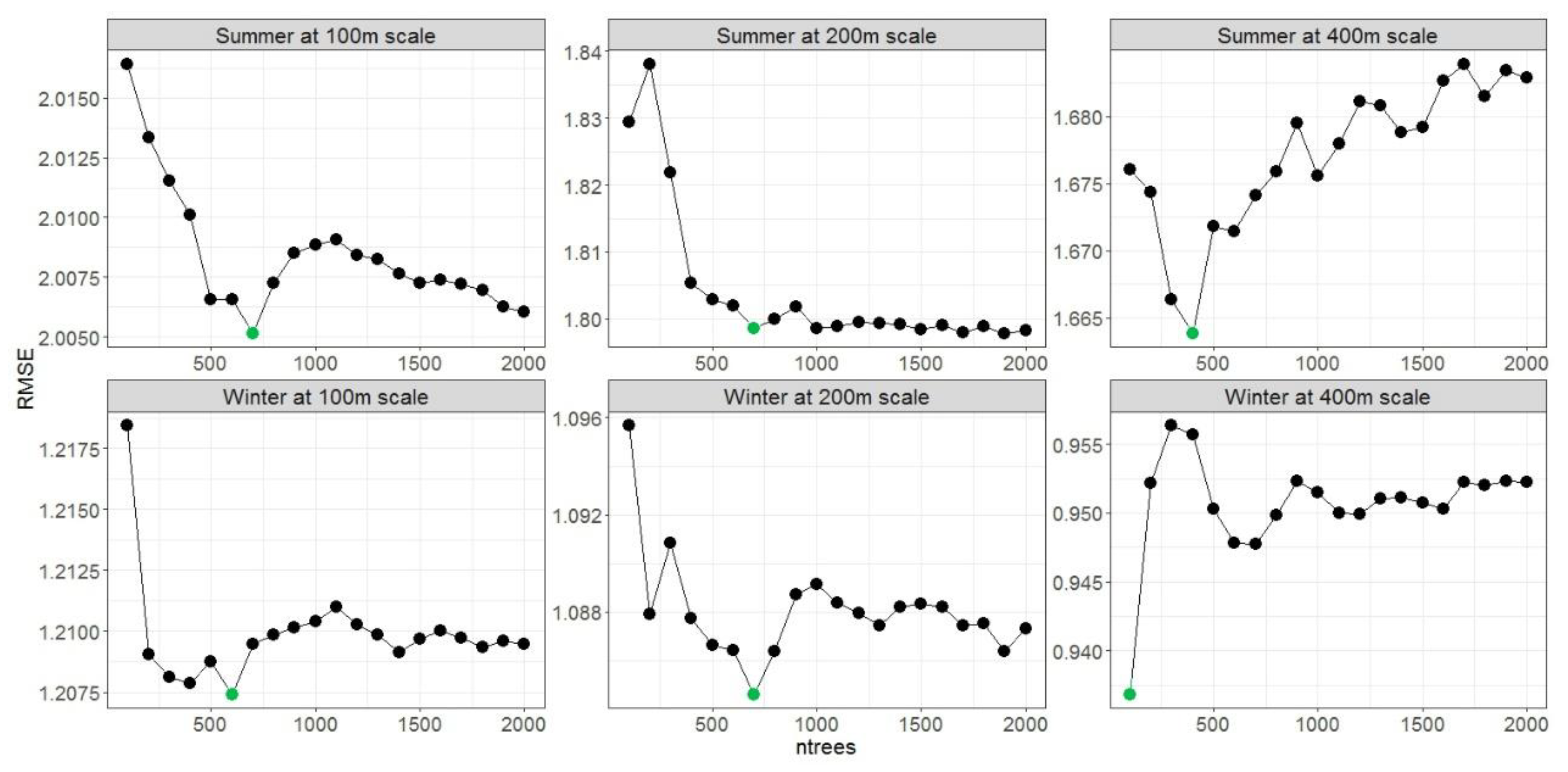
Unlike many other nonlinear estimators, RF does not require a split-sampling method to assess the accuracy of the model [38]. Repeated 10-fold cross-validation (CV) was conducted to evaluate the validity of RF models using the same observation dataset. The validation dataset was built by randomly selecting 10% out of all observation samples and the rest of the 90% were used as the training dataset. This process was repeated 10 times. The overall adjusted R2 and Root Mean Square Error (RMSE) were calculated. The statistical parameters of R2, MAE, and RMSE were then calculated using 10-fold cross-validation results and were used to compare the performance of the RF models in different seasons and observation scales. To find the optimal ntrees values that can best predict the urban LST, the ntrees values were tested from 100 to 2000 with intervals of 100. Finally, the random forest was optimized for the best value of ntrees based on the lowest Root Mean Square Error (RMSE) (Figure 5).
3. Results
3.1. Spatial Distribution Patterns and Seasonal Characteristics of LST
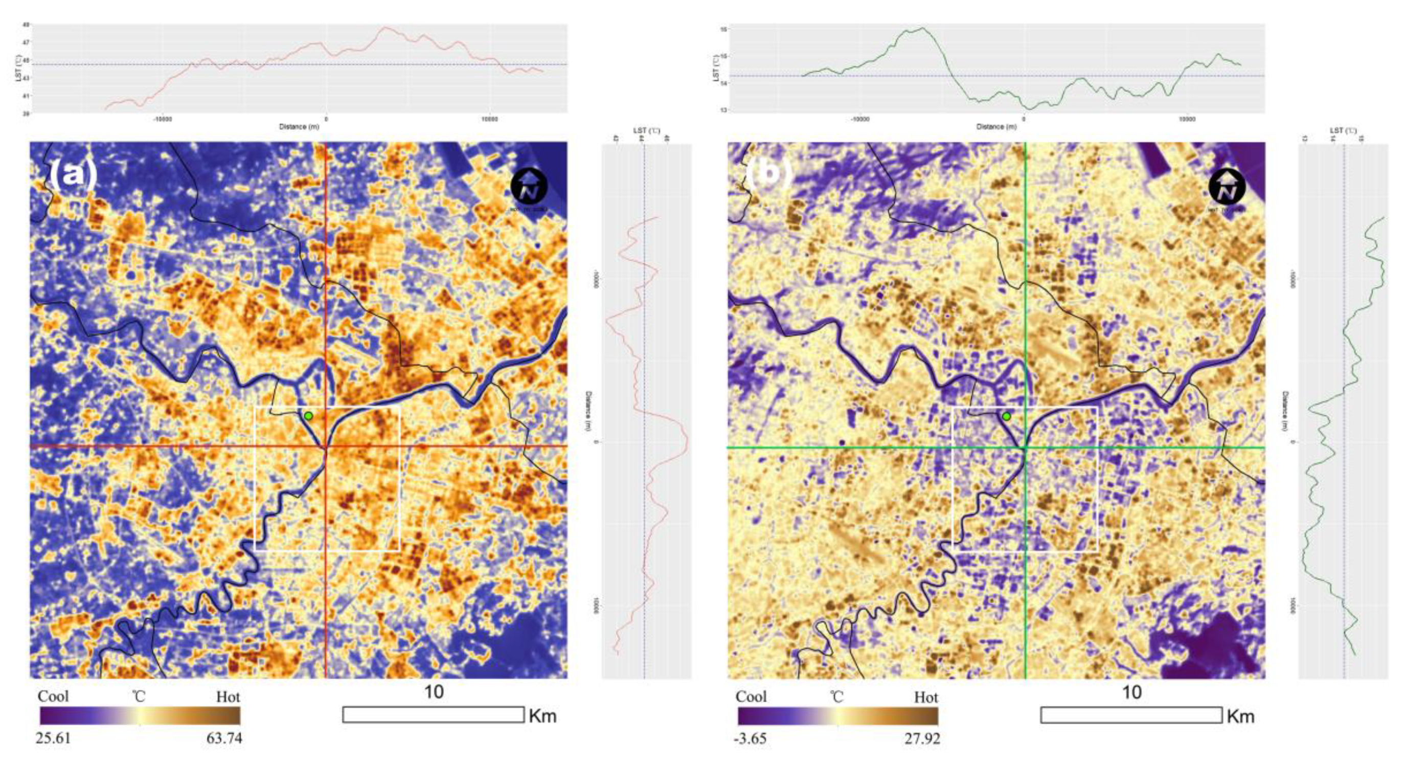
The descriptive statistics of the LST for both summer and winter in the study area were illustrated in Table 1. In our study area, within the extent of 8 km × 8 km, the average LST at 10:55 in summer reached up to 45.88 °C, whereas in winter it was only 13.9 °C. In addition, LST in winter had a higher coefficient of variation (CV) than in summer, which indicated that temperature fluctuation in winter was more dramatic than in summer. Figure 6 shows the spatial distribution of LST in both summer and winter. It clearly demonstrated that the urban center area (the white rectangle in the figure) exhibited a significant UHI effect in the summer day, while it presented a clear urban cold island effect in the winter day. The LST profiles in both the horizontal and vertical directions exhibited the larger spatial variability of LST along the urban-rural gradients of Ningbo City. In summer, the mean LSTs reached their peaks at the location of near urban center, and the mean LST of the study area was 2~3 °C higher than that of surrounding areas. In winter, an opposite trend was observed; the mean LST of the study area was about 1 °C lower than that of surrounding areas.
3.2. Model Estimation and Validation
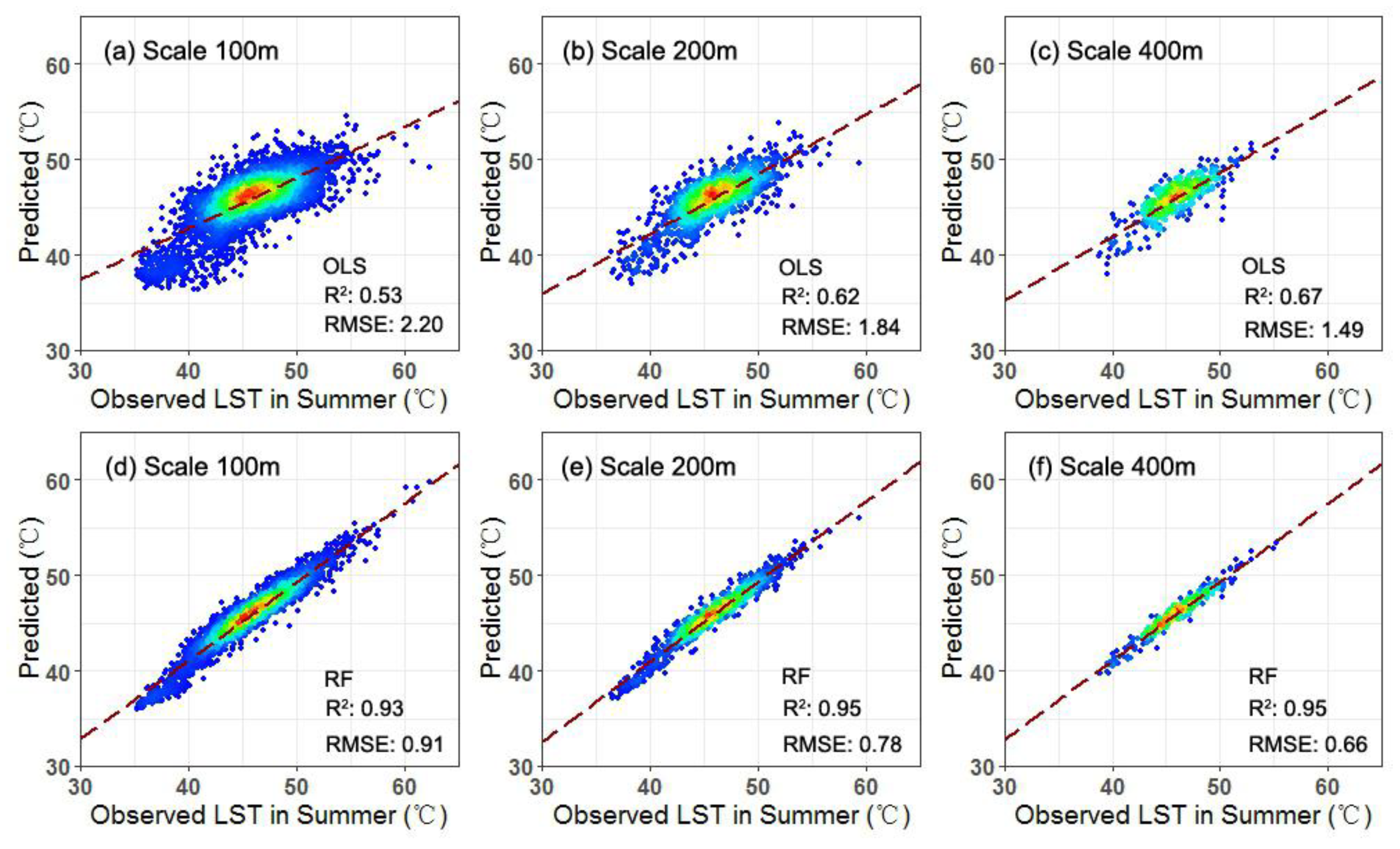
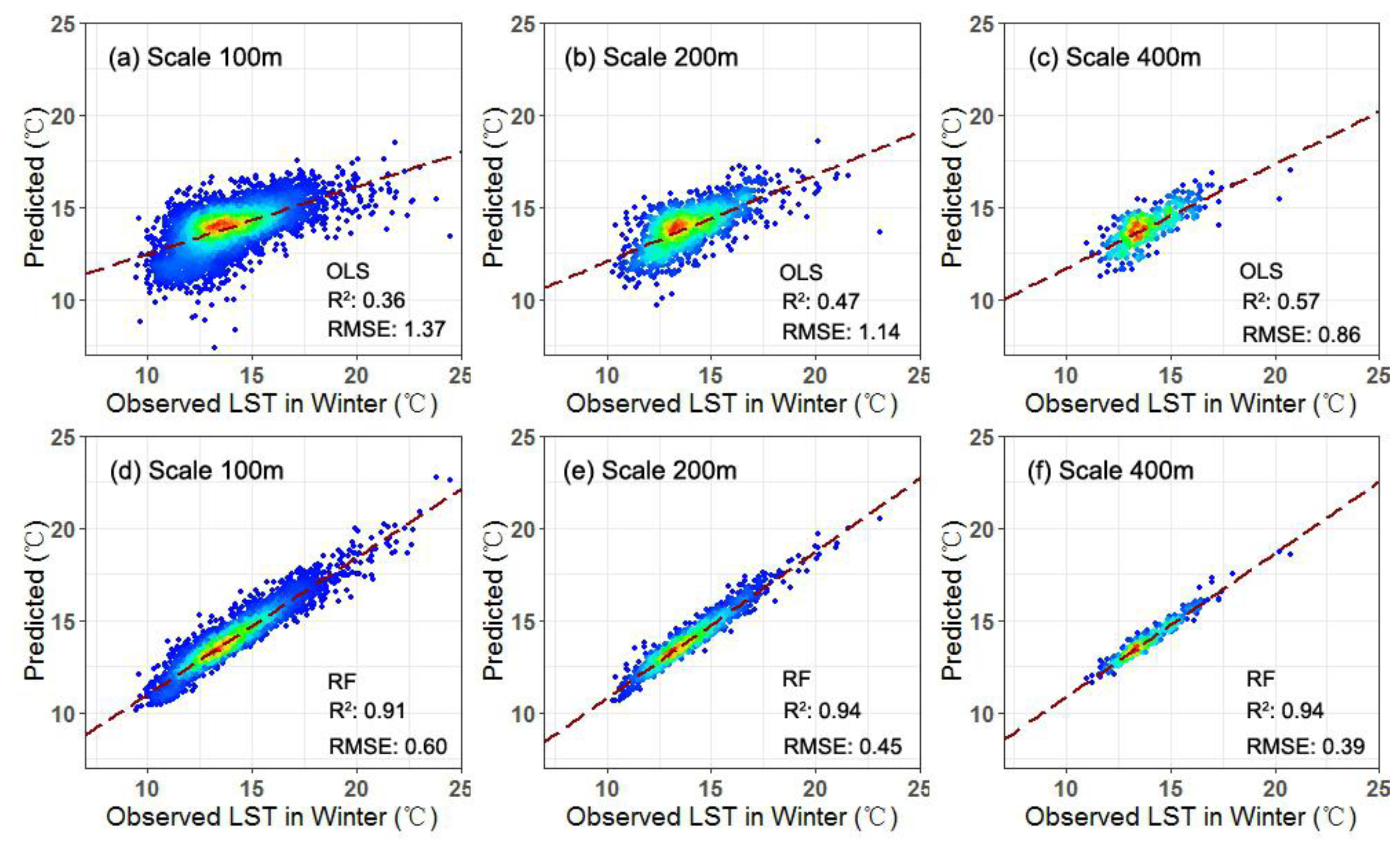
Figure 7 and Figure 8 show the model performances for OLS and RF in both summer and winter. All seven urban form metrics were considered in the model estimation process. At the three observation scales, the OLS regression models explained 53%~67% (RMSE = 2.20 °C, 1.84 °C, 1.49 °C for the 100 m, 200 m, and 400 m grids) of the LST in summer, and captured 36%~57% (RMSE = 1.37 °C, 1.14 °C, 0.86 °C for the 100 m, 200 m, and 400 m grids) of the LST in winter. However, the RF regression models showed a significant improvement compared with the OLS models. All RF models have higher R2 (>0.9) and lower RMSE/MAE values. Regarding the values of RMSE, both the OLS and RF models have slightly higher performances in winter than in summer, which seems to relate to the much larger dynamic range of summer LST than winter LST. In addition, the explanatory power of the OLS and RF models always increased with the extending of the observation grid size, which mainly attributes to higher sensibility to the neighboring environment for small grids than large grids [27].
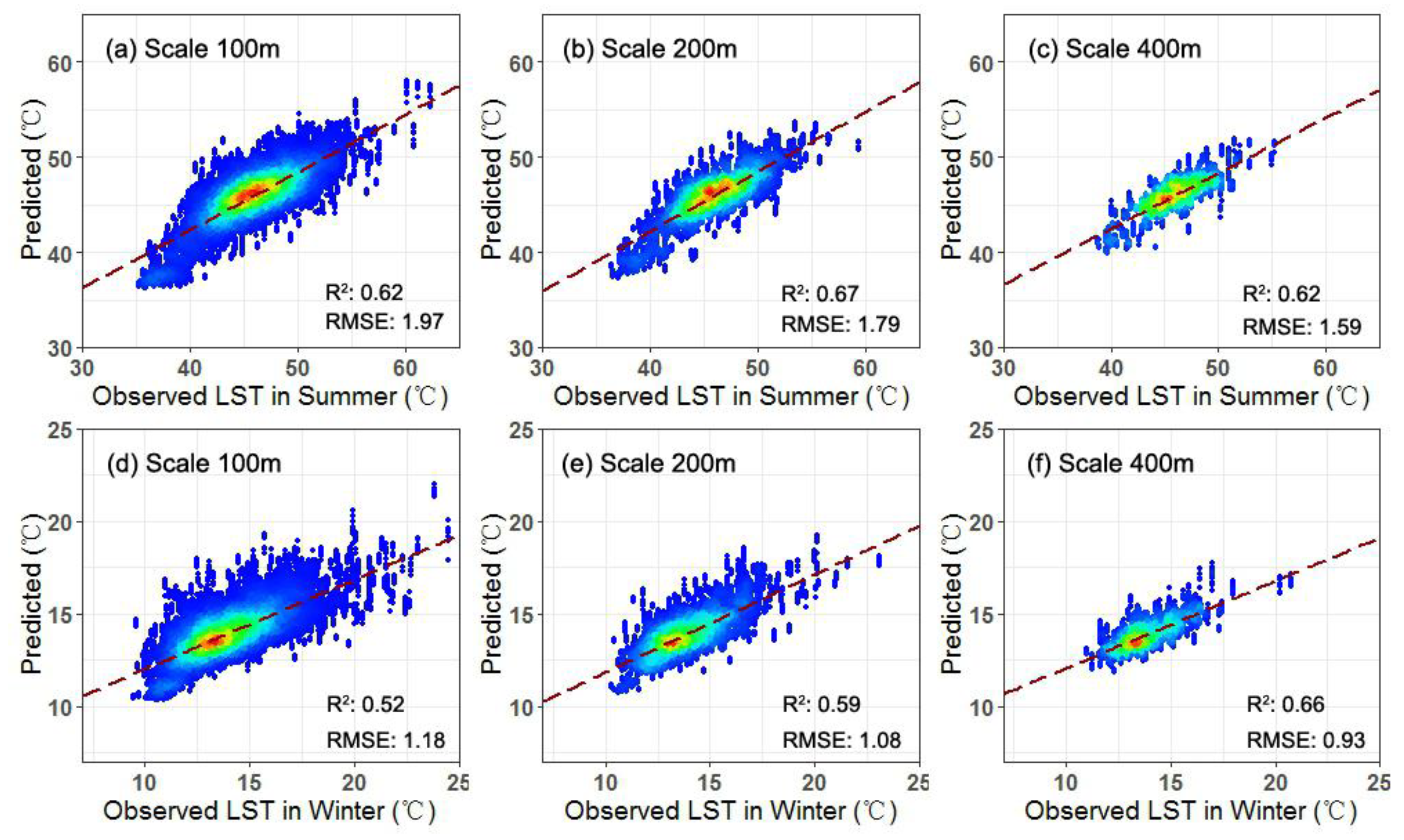
To further evaluate the predictive abilities of the RF models to LST, the repeated 10-fold cross-validation (CV) method was adopted. Scatter plots of the predicted and observed values obtained from CV are presented in Figure 9. The statistical indicators of R2 and RMSE showed robust predictive abilities and modest prediction errors with little bias. The best predictive performance was observed for the winter LST estimation at the 400 m grid (CV R2 = 0.66, RMSE = 0.93 °C). Overall, higher-level predictions showed in winter and coarser observation scales.
3.3. Impact of Urban Form Metrics on the LST
The results from the step-wise RF regression analysis were shown in Table 2, which could examine to what degree each urban form metrics explain the LST variations. When considering all five urban form aspects, more than 60% of the LST variations in summer could be explained, and more than 50% of those in winter. Urban ecological infrastructure was identified as the most important contributor, with the relative explanation rate of almost 70% in summer and 40% in winter. The second largest contributor was the building morphology, which has the relative explanation rate of almost 15% in summer and 40% in winter. The aspects of transportation systems, human activity, and public infrastructure seem to have a limited impact on the LST variations. Most of the relative explanation rate for them were lower than 10%, which confirmed their relatively-lower effect on the overall model performance.
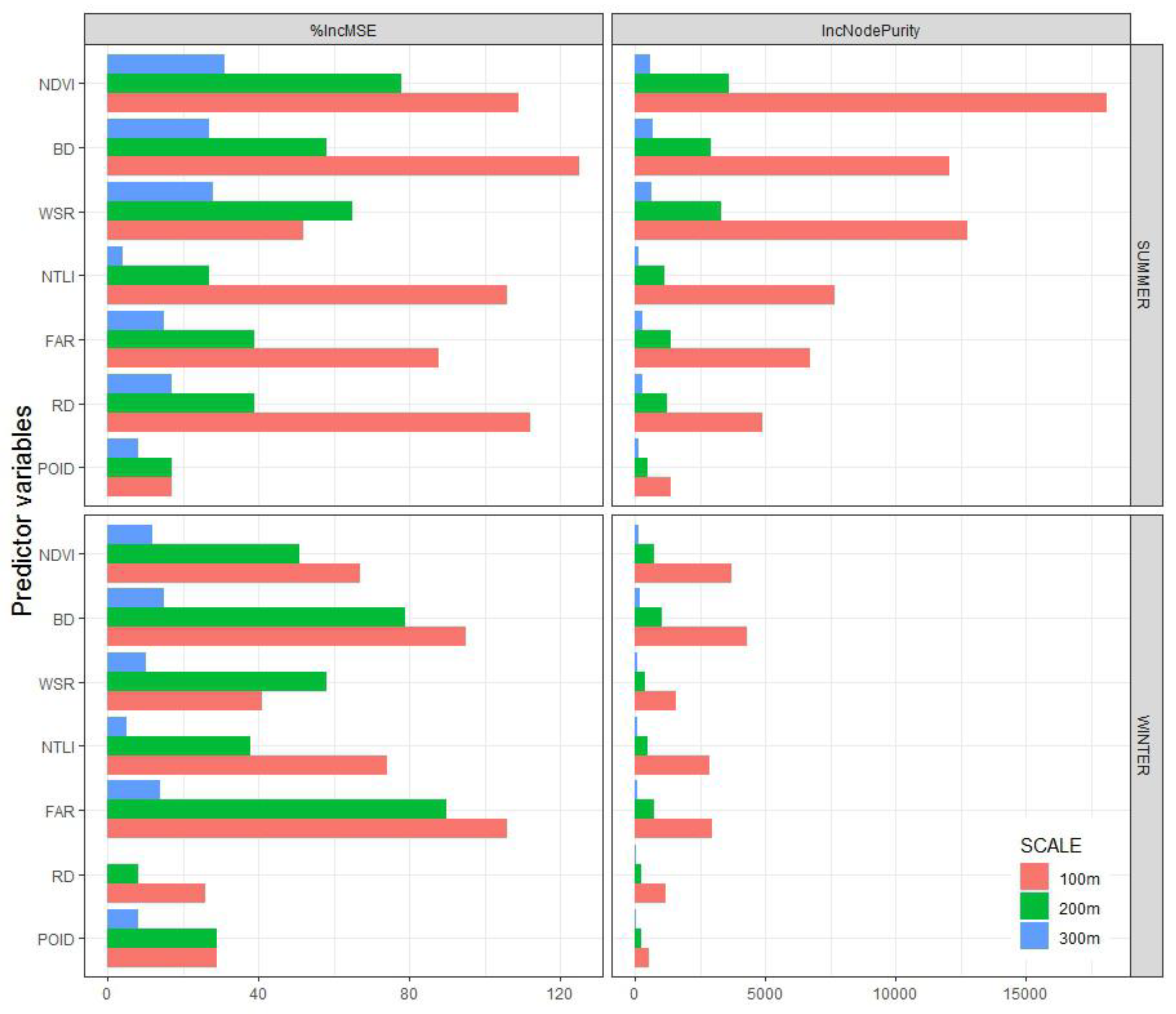
RF models computed two qualitative measures that describe the relative importance of the predictor variables: The Increased Mean Square Error (%IncMSE) and Increased Impurity Index (IncNodePurity) [39]. Figure 10 shows the relative variable importance ranking for both multiple observation scales and summer–winter seasons. Based on the average rankings of both %IncMSE and IncNodePurity, the urban ecological infrastructure metrics (NDVI) and building features metrics (BD) were the most influential variables for determining the LST variations across the study area. There was a decline in importance ranking for the metrics of WSR, NTLI, and FAR. The rest of the variables like the RD and POID have relatively small importance to LST in both summer and winter. The importance of the seven independent variables varied with the changes of observation scale and season. When the temperature was high in summer, LST variations were more likely controlled by ecological infrastructure factors in high-density urban center. The effects of ecological infrastructure factors on low LST in winter weakened, while the building feature factors converted to the dominant factor.
The OLS regression results for LST and its factors of influence are shown in Table 3, which facilitates the identification of the effect of the magnitude and direction of urban form on the LST variations. Two urban form aspects, ecological infrastructure and building morphology, were identified as the dominant factors for the change of LST. Such results are consistent with the variable importance measures from the RF.
Firstly, the coefficients of two ecological infrastructure metrics (NDVI and WSR) in all models were significantly negative with LST in summer and winter. This confirmed that green space and water body in urban areas have cooling effects through evaporation and shading in both hotter and cooler months. Such cooling effect was stronger in summer than in winter, and decreased with an increasing grid size. These results were consistent with the variable importance measures in Section 3.3, and the previous findings reported by Peng et al. [40].
Secondly, two building feature metrics, BD and FAR, showed the opposite impact on the LST variations. In detail, BD had a positive influence on the LST, while FAR had a negative influence. This is consistent with the findings reported by Lin et al. [41], Yin et al. [14], and Cai et al. [13]. Building density is closely related to air flow, that is, high building density weakens the ventilation conditions resulting in high thermal environment. On the other hand, high-rise urban areas that have higher FAR may produce a large amount of shadows, which results in a lower LST. In general, the urban areas with sparse buildings and high-rise buildings tend to be cooler.
Thirdly, road density (RD) always has a positive effect on LST, and most of such correlations were significant except in winter at the 400 m grid, which means that urban areas with high levels of accessibility would be hotter than low RD areas. However, the impact of RD on LST variations were very weak throughout the year.
Fourthly, the nighttime light intensity (NTLI), as a proxy for human activities intensity and night-time population distribution, has a negative effect on LST in most cases, but only significant correlations with LST variation in winter. However, POI density (POID), as another human activity metric, always has a significant negative correlation. According to the coefficients of two indicators, the POID may have a stronger impact on LST than that for NTLI. This human activities effect may be explained as follows: (1) Inconsistency between daytime and nighttime population distribution. The negative effect of the NTLI variable on LST would attribute to the phenomena of “home–work separation” [42], which may result in the opposite spatial patterns between daytime LST and nighttime light intensity. (2) Geographical features of Ningbo City. As shown in Figure 1, Ningbo is a typically intensive river network zone, especially in the urban center. For this study, high-density public infrastructure POI was located along both sides of the river. Thus, anthropogenic heat emissions yielding by human activity were offset by the stronger cooling effect of the water body.
4. Discussion
4.1. Urban Form and LST
Numerous previous studies have acknowledged that urban form metrics significantly affect urban thermal environments. In a perspective of urban physical space hierarchy, we redefine and disassemble the urban form into five aspects: Building morphology, transportation system, public infrastructure, ecological infrastructure, and human activity. Employing the OLS and RF regression analysis methods demonstrated the different effects of urban form characteristics on summer and winter LST. Both of the coefficients of OLS models and step-wise RF models outputs suggested that the LST variations were dominated by the urban ecological and building composition, while the other urban form metrics, like transportation system, public infrastructure, and human activity presented a relatively weak contribution to the LST variations. Similar laws also were obtained for Shenzhen [40], Shanghai [20], and Wuhan City [13].
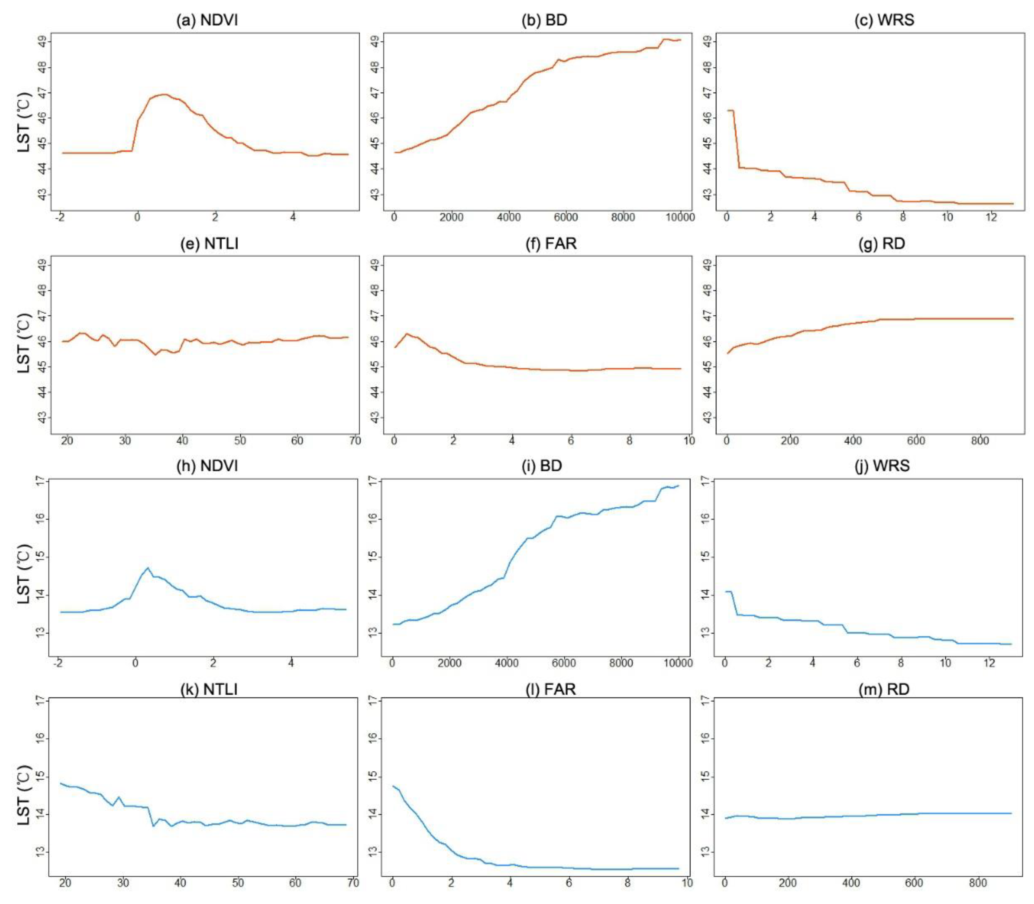
In the Ningbo urban center, the mean LST was associated negatively with the area occupied by vegetation and water bodies. The partial dependence plot for NDVI and WSR illustrated a clear trend of LST decrease (Figure 11a,c,h,j) in both summer and winter. However, when the values of NDVI and WSR were larger than 3 and 8% respectively, the decline in LST slowed down. With respect to urban building morphology metrics, the LST was positively related with the BD but negatively related with the FAR (Figure 10b,i). Similar to the trends of NDVI and WSR, the LST decreased dramatically with increasing FAR (Figure 11f,l). These results reflected the complex correlations between the LST and urban form metrics. NTLI and RD exhibited a relatively weak influence on the LST.
In other word, we can also concluded that the planning and update of key components on urban surfaces, such as green spaces, water bodies, and buildings, would have a stronger impact on the LST. However, normal population migration and redistribution of public infrastructure may have a small impact on the LST variations. Therefore, urban planners and managers of Ningbo City should pay more attention on the arrangement of buildings and ecological compositions in the high-density urban center, rather than the restriction of related human activities, in order to improve the urban thermal environment and mitigate the UHI effect.
4.2. Seasonal and Scale Effects
In this study, the results from quantitative analysis indicated that both seasonal and scale effects exist in the correlations between urban form metrics and LST. The LST and their correlations with urban form metrics has shown significant seasonal variations and large differences between summer and winter. The urban form has a closer correlation with LST in summer than in winter. Modelling results also indicated the prominent LST variations in summer were controlling by urban ecological infrastructure, while these variations in winter were effectively linked to urban ecological infrastructure and building features. As a subtropical coastal city, Ningbo’s temperature fluctuation in winter was more extreme, and was affected by many other factors. The cooling effects of green spaces and water bodies were much stronger in summer. In contrast, building features had relatively weak effects in summer.
The UHI effect and its influencing factors are always sensitive to changes in grid size [43]. Considering the average urban block scale in Ningbo city, three observation scales were selected in this study: 100 m, 200 m, and 400 m. In general, the explanatory power for both the OLS and RF regression increased from small grids to coarse grids. The best regression results were obtained with the 400 m grid, which indicated that using larger cells would be able to better capture urban form effects. In addition, the coefficient in absolute value of two ecological infrastructure metrics (NDVI and WSR) decreased with an increasing grid size, whereas the coefficient of FAR increased, in absolute value, from smaller to larger grids. Cai et al. [44] found a similar conclusion in central Beijing. Thus, we suggest that the larger observation scale closing to the biggest local block size (with the grid size of 200~400 m) was more suitable for exploring the effects of urban form on the LST.
5. Conclusions
Taking the subtropical coastal city of Ningbo as a case study, this work quantitatively examined the relative contributions of urban form metrics on the LST variations in both summer and winter using OLS and RF ensemble models. Firstly, urban form was redefined and disassembled into five aspects by fully considering the urban physical spatial structures. Subsequently, seven urban form metrics were selected according to the availability of spatial data and representative principle. Finally, we constructed the OLS and RF regression models for a high-density urban area with the size of 8 km × 8 km to distinguish to what degree each urban form metric influenced the LST patterns. The RF models were verified using rigorous repeated 10-cross-validation procedures, which results demonstrated that RF provides superior performance in modelling the complex nonlinear relationships between urban form and LST variations.
The outcomes of this study indicated that the urban form could explain more than 90% of the variance LST in summer and winter using RF. Among the five aspects of urban form metrics, urban ecological infrastructure was identified as the dominant contributor of cooling effects. Building morphology ranked in the second place. Specifically, the LST was positively related with the BD but negatively related with the FAR. However, the other aspects, transportation system, human activity, and public infrastructure, seem to have a limited impact on the LST variations. In addition, urban form metrics’ impact on the LST has shown significant seasonal and observation scale variations. The cooling effects of green spaces and water bodies were much stronger in summer, while the building morphology had relatively weak effects in summer. The best modelling results were generally obtained at the 400 m grid, which was found to be the ideal observation scale to explore the correlations between the LST and urban form in the high-density urban areas.
This study confirmed that the reconstruction and update of urban ecological infrastructure and buildings would have a stronger impact on the changes of LST, while construction of transportation, normal population migration, and redistribution of public infrastructure may have a small impact on the LST. Therefore, urban planners and managers should pay more attention to the arrangement of buildings and ecological compositions in high-density urban centers, rather than related human activities, in order to improve the urban thermal environment. We also suggest that the construction of high-rise and low-density urban buildings may be an effective measure to create a comfortable outdoor thermal environment, apart from increasing the coverage rate of vegetation and water bodies. Our empirical findings on the dependence of the LST on the urban form could be given to urban planners and managers for land-use management and UHI mitigation from a microcosmic perspective. Further research might take the dynamics of urban form and more additional factors into consideration.
Author Contributions
S.Y. analyzed the data and wrote the paper; G.C. designed the experiments; the other author contributed to the materials/analysis tools.
Funding
This work was sponsored by K.C. Wong Magna Fund in Ningbo University and the National Natural Science Foundation of China (41571018) and (41871024).
Acknowledgments
The authors are thankful to the anonymous reviewers who provided constructive comments to improve this manuscript.
Conflicts of Interest
The authors declare no conflict of interest.
References
- Peng, S.; Piao, S.; Ciais, P.; Friedlingstein, P.; Ottle, C.; Bréon, F.M.; Nan, H.; Zhou, L.; Myneni, R.B. Surface urban heat island across 419 global big cities. Environ. Sci. Technol. 2012, 46, 696–703. [Google Scholar] [CrossRef]
- Oke, T.R. The energetic basis of the urban heat island. Quart. J. Royal Meteorol. Soc. 1982, 108, 1–24. [Google Scholar] [CrossRef]
- Grimm, N.B.; Faeth, S.H.; Golubiewski, N.E.; Redman, C.L.; Wu, J.G.; Bai, X.M.; Briggs, J.M. Global change and the ecology of cities. Science 2008, 319, 756–760. [Google Scholar] [CrossRef]
- Jenerette, G.D.; Harlan, S.L.; Buyantuev, A.; Stefanov, W.L.; Declet-Barreto, J.; Ruddel, B.L.; Myint, S.W.; Kaplan, S.; Li, X.X. Micro-scale urban surface temperatures are related to land-cover features and residential heat related health impacts in Phoenix, AZ USA. Landsc. Ecol. 2016, 31, 745–760. [Google Scholar] [CrossRef]
- Li, H.D.; Meier, F.; Lee, X.H.; Chakraborty, T.; Liu, J.F.; Schaap, M.; Sodoudi, S. Interaction between urban heat island and urban pollution island during summer in Berlin. Sci. Total Environ. 2018, 636, 818–828. [Google Scholar] [CrossRef]
- Liu, J.; Cheng, H.; Jiang, D.; Huang, L. Impact of climate-related changes to the timing of autumn foliage colouration on tourism in Japan. Tour. Manage. 2019, 70, 262–272. [Google Scholar] [CrossRef]
- Liu, J.; Wang, J.; Wang, S.H.; Wang, J.F.; Deng, G.P. Analysis and simulation of the spatiotemporal evolution pattern of tourism lands at the Natural World Heritage Site Jiuzhaigou, China. Habitat Int. 2018, 79, 74–88. [Google Scholar] [CrossRef]
- Burke, M.; González, F.; Baylis, P.; Heft-Neal, S.; Baysan, C.; Basu, S.; Hsiang, S. Higher temperatures increase suicide rates in the United States and Mexico. Nat. Clim. Change 2018, 8, 723–729. [Google Scholar] [CrossRef]
- Zhou, X.F.; Chen, H. Impact of urbanization-related land use land cover changes and urban morphology changes on the urban heat island phenomenon. Sci. Total Environ. 2018, 635, 1467–1476. [Google Scholar] [CrossRef]
- Zhou, B.; Rybski, D.; Kropp, J.P. The role of city size and urban form in the surface urban heat island. Sci. Rep. 2017, 7, 4791. [Google Scholar] [CrossRef] [PubMed] [Green Version]
- Wentz, E.A.; York, A.M.; Alberti, M.; Conrow, L.; Fischer, H.; Inostroza, L.; Jantz, C.; Pickett, S.T.A.; Seto, K.C.; Taubenböck, H. Six fundamental aspects for conceptualizing multidimensional urban form: A spatial mapping perspective. Landsc. Urban Plan. 2018, 179, 55–62. [Google Scholar] [CrossRef]
- Taleghani, M.; Kleerekoper, L.; Tenpierik, M.; Dobbelsteen, A. Outdoor thermal comfort within five different urban forms in the Netherlands. Build. Environ. 2015, 83, 65–78. [Google Scholar] [CrossRef]
- Cai, Z.; Han, G.F.; Chen, M.C. Do water bodies play an important role in the relationship between urban form and land surface temperature? Sustain. Cities Soc. 2018, 39, 487–498. [Google Scholar] [CrossRef]
- Yin, C.H.; Yuan, M.; Lu, Y.P.; Huang, Y.P.; Liu, Y.F. Effects of urban form on the urban heat island effect based on spatial regression model. Sci. Total Environ. 2018, 634, 696–704. [Google Scholar] [CrossRef]
- Middel, A.; Häb, K.; Brazel, A.J.; Martin, C.A.; Guhathakurta, S. Impact of urban form and design on mid-afternoon microclimate in Phoenix Local Climate Zones. Landsc. Urban Plan. 2014, 122, 16–28. [Google Scholar] [CrossRef] [Green Version]
- Alobaydi, D.; Bakarman, M.A.; Obeidat, B. The Impact of Urban Form Configuration on the Urban Heat Island: The Case Study of Baghdad, Iraq. Procedia Eng. 2016, 145, 820–827. [Google Scholar] [CrossRef]
- Yang, J.; Sun, J.; Ge, Q.S.; Li, X.M. Assessing the Impacts of Urbanization-Associated Green Space on Urban Land Surface Temperature: A Case Study of Dalian, China. Urban For. Urban Gree. 2017, 22, 1–10. [Google Scholar] [CrossRef]
- Yang, J.; Guan, Y.Y.; Xia, J.H. (Cecilia); Jin, C.; Li, X.M. Spatiotemporal variations in greenspace ecosystem service value at urban fringes: A case study on Ganjingzi District in Dalian, China. Sci. Total Environ. 2018, 639, 1453–1461. [Google Scholar] [CrossRef]
- Yang, J.; Guo, A.D.; Li, Y.H.; Zhang, Y.Q.; Li, X.M. Simulation of landscape spatial layout evolution in rural-urban fringe areas: a case study of Ganjingzi District. Gisci. Remote Sens. 2019, 56, 388–405. [Google Scholar] [CrossRef]
- Sun, Y.W.; Gao, C.; Li, J.L.; Li, W.F.; Ma, R.F. Examining urban thermal environment dynamics and relations to biophysical composition and configuration and socio-economic factors: A case study of the Shanghai metropolitan region. Sustain. Cities Soc. 2018, 40, 284–295. [Google Scholar] [CrossRef]
- Tran, D.X.; Pla, F.; Latorre-Carmona, P.; Myint, S.W.; Caetano, M.; Kieu, H.V. Characterizing the relationship between land use land cover change and land surface temperature. ISPRS J. Photogramm. 2017, 124, 119–132. [Google Scholar] [CrossRef] [Green Version]
- Padmanaban, R.; Bhowmik, A.K.; Cabra, P.l. Satellite image fusion to detect changing surface permeability and emerging urban heat islands in a fast-growing city. PLoS ONE 2019, 14, e0208949. [Google Scholar] [CrossRef]
- Oleson, K.W.; Monaghan, A.; Wilhelmi, O.; Barlage, M.; Brunsell, N.; Feddema, J.; Hu, L.; Steinhoff, D.F. Interactions between urbanization, heat stress, and climate change. Clim. Chang. 2015, 129, 525–541. [Google Scholar] [CrossRef]
- Guo, G.; Zhou, X.; Wu, Z.; Xiao, R.; Chen, Y. Characterizing the impact of urban morphology heterogeneity on land surface temperature in Guangzhou, China. Environ. Model Softw. 2016, 84, 427–439. [Google Scholar] [CrossRef]
- Giridharan, R.; Lau, S.S.Y.; Ganesan, S. Nocturnal heat island effect in urban residential developments of Hong Kong. Energ. Buildings 2005, 37, 964–971. [Google Scholar] [CrossRef]
- Chun, B.; Guldmann, J.M. Spatial statistical analysis and simulation of the urban heat island in high-density central cities. Landsc. Urban Plan. 2014, 125, 76–88. [Google Scholar] [CrossRef]
- Chun, B.; Guldmann, J.M. Impact of greening on the urban heat island: Seasonal variations and mitigation strategies. Comput. Environ. Urban 2018, 71, 165–176. [Google Scholar] [CrossRef]
- Yang, J.; Jin, S.H.; Xiao, X.M.; Jin, C.; Xia, J.H. (Cecilia); Li, X.M.; Wang, S.J. Local Climate Zone Ventilation and Urban Land Surface Temperatures: Towards a Performance-based and Wind-sensitive Planning Proposal in Megacities. Sustain. Cities Soc. 2019, 47, 1–11. [Google Scholar] [CrossRef]
- Yang, J.; Su, J.R.; Xia, J.H. (Cecilia); Jin, C.; Li, X.M.; Ge, Q.S. The Impact of Spatial Form of Urban Architecture on the Urban Thermal Environment: A Case Study of the Zhongshan District, Dalian, China. IEEE J. Sel. Top. Appl. Earth Obs. Remote Sens. 2018, 11, 2709–2716. [Google Scholar] [CrossRef]
- Tang, Y.T.; Chan, F.K.S.; Griffiths, J. City profile: Ningbo. Cities 2015, 42, 97–108. [Google Scholar] [CrossRef] [Green Version]
- Zhao, Y.C.; Zhao, X.F.; Da, K. Multi-index Analysis of Heat Island Dynamics with the Process of Urbanisation in Ningbo City. Ecol. Environ. Sci. 2014, 23, 1628–1635. [Google Scholar]
- Artis, D.A.; Carnahan, W.H. Survey of emissivity variability in thermography of urban areas. Remote Sens. Environ. 1982, 12, 313–329. [Google Scholar] [CrossRef]
- Weng, Q.; Lu, D.; Schubring, J. Estimation of land surface temperature-vegetation abundance relationship for urban heat island studies. Remote Sens. Environ. 2004, 89, 467–483. [Google Scholar] [CrossRef]
- Huang, Y.P.; Sun, Y.M. Judgment Characteristics and Quantitative Index of Suitable Block Scale. J. South China Univ. Technol. 2012, 40, 131–138. [Google Scholar]
- Huang, W.F.; Ding, J.Y.; Dan, M. The historical evolution of urban block scale—taking Ningbo as an example. In Proceeding of Annual meeting of China’s urban planning, Shenyang, China, 24 September 2016. [Google Scholar]
- Breiman, L. Random forests. Mach. Learn. 2001, 45, 5–32. [Google Scholar] [CrossRef]
- Liaw, A.; Wiener, M. Classification and regression by random Forest. R News 2002, 2, 18–22. [Google Scholar]
- Ehrlinger, J. ggRandomForests: Random Forests for Regression. arXiv, 2014; arXiv:1501.07196. [Google Scholar]
- Gregorutti, B.; Michel, B.; Saint-Pierre, P. Correlation and variable importance in random forests. Stat. Comput. 2017, 27, 659–678. [Google Scholar] [CrossRef]
- Peng, J.; Jia, J.L.; Liu, Y.X.; Li, H.L.; Wu, J.S. Seasonal contrast of the dominant factors for spatial distribution of land surface temperature in urban areas. Remote Sens. Environ. 2018, 215, 255–267. [Google Scholar] [CrossRef]
- Lin, P.; Siu, S.; Qin, H.; Gou, Z. Effects of urban planning indicators on urban heat island: A case study of pocket parks in high-rise high-density environment. Landsc. Urban Plan. 2017, 168, 48–60. [Google Scholar] [CrossRef]
- Qi, W.; Li, Y.; Liu, S.H.; Gao, X.L.; Zhao, M.F. Estimation of urban population at daytime and nighttime and analyses of their spatial pattern: A case study of Haidian District, Beijing. Acta Geograph. Sin. 2013, 68, 1344–1356. [Google Scholar]
- Yang, J.; Wang, Y.C.; Xiao, X.M.; Jin, C.; Xia, J.H. (Cecilia); Li, X.M. Spatial Differentiation of Frontal Area Index and Land Surface Temperature in Different Grid Sizes. Urb. Clim. 2019, 28, 1–13. [Google Scholar] [CrossRef]
- Dai, Z.X.; Guldmann, J.; Hu, Y.F. Spatial regression models of park and land-use impacts on the urban heat island in central Beijing. Sci. Total Environ. 2018, 626, 1136–1147. [Google Scholar]
Figure 1.
Location of the study area. (a) Ningbo City and its administrative boundaries; (b) Landsat 8 image on 23 July 2017 displayed in color composition RGB with bands 7, 6, and 4; the yellow rectangle represented the study area in this paper.
Figure 1.
Location of the study area. (a) Ningbo City and its administrative boundaries; (b) Landsat 8 image on 23 July 2017 displayed in color composition RGB with bands 7, 6, and 4; the yellow rectangle represented the study area in this paper.

Figure 2.
Violin plot of the monthly average temperature of Yinzhou weather station in Ningbo City during 1980–2010.
Figure 2.
Violin plot of the monthly average temperature of Yinzhou weather station in Ningbo City during 1980–2010.

Figure 3.
Conceptual relationship graphs of the five aspects of urban form.

Figure 4.
Selected urban form metrics in this study. (a) Road network; (b) POI; (c) NTL; (d) Building height; (e) NDVI.
Figure 4.
Selected urban form metrics in this study. (a) Road network; (b) POI; (c) NTL; (d) Building height; (e) NDVI.

Figure 5.
Optimization of random forest parameters (number of trees in the forest (ntrees) using Root Mean Square Error (RMSE). The optimal ntrees that was selected with the lowest RMSE is shown with the green spots.
Figure 5.
Optimization of random forest parameters (number of trees in the forest (ntrees) using Root Mean Square Error (RMSE). The optimal ntrees that was selected with the lowest RMSE is shown with the green spots.

Figure 6.
Land surface temperature in Ningbo City: (a) Summer; (b) winter. The white rectangle represents the study area in this paper. The LST profiles in both horizontal and vertical directions are also presented on the top and right of each figure.
Figure 6.
Land surface temperature in Ningbo City: (a) Summer; (b) winter. The white rectangle represents the study area in this paper. The LST profiles in both horizontal and vertical directions are also presented on the top and right of each figure.

Figure 7.
Density scatter plots between predicted and observed LST in summer from both the ordinary least-squares (OLS) and random forest regression (RF) model fittings. The color ramp from blue to red corresponds to increasing point density. Red dashed lines represent the regression line. (a), (b), and (c) are plots at the 100m, 200m, and 400m scales for the OLS model, respectively; (d), (e), and (f) are plots at the 100m, 200m, and 400m scales for the RF model, respectively.

Figure 8.
Density scatter plots between predicted and observed LST in winter from both the OLS and RF model fittings. (a), (b), and (c) are plots at the 100m, 200m, and 400m scales for the OLS model, respectively; (d), (e), and (f) are plots at the 100m, 200m, and 400m scales for the RF model, respectively.

Figure 9.
Density scatter plots between predicted and observed LST from repeated 10-fold cross validation results based on the final RF models. (a), (b), and (c) are plots at the 100m, 200m, and 400m scales for the OLS model, respectively; (d), (e), and (f) are plots at the 100m, 200m, and 400m scales for the RF model, respectively.

Figure 10.
Relative variable importance calculated from the final RF models.

Figure 11.
Partial dependence plots for the dominant variables in summer (a)–(g) and winter (h)–(m). The partial plots show the dependencies of the LST on each of the predictors.
Figure 11.
Partial dependence plots for the dominant variables in summer (a)–(g) and winter (h)–(m). The partial plots show the dependencies of the LST on each of the predictors.


Table 1.
Descriptive statistics of the land surface temperature LST for both summer and winter in the study area (°C).
Table 1.
Descriptive statistics of the land surface temperature LST for both summer and winter in the study area (°C).
| Seasons | Mean | Min. | Max. | Std. dev. | CV (%) |
|---|---|---|---|---|---|
| Summer (23/07/2017) | 45.88 | 35.20 | 62.34 | 3.22 | 7.02 |
| Winter (03/02/2017) | 13.9 | 9.42 | 26.29 | 1.71 | 12.32 |
Table 2.
Summaries of the explanatory power for each urban form aspect using the step-wise RF regression models.
Table 2.
Summaries of the explanatory power for each urban form aspect using the step-wise RF regression models.
| Categories | Summer | Winter | ||||
|---|---|---|---|---|---|---|
| Scale 100 m | Scale 200 m | Scale 400 m | Scale 100 m | Scale 200 m | Scale 400 m | |
| Ecological infrastructure | 42.31(67.59) | 47.95(73.01) | 48.56(74.35) | 20.87(39.86) | 21.68(38.47) | 24.11(44.35) |
| Building morphology | 8.75(13.98) | 10.03(15.27) | 10.37(15.88) | 20.38(38.92) | 26.51(47.05) | 24.59(45.24) |
| Transportation system | 4.05(6.47) | 2.86(4.35) | 0.15(0.23) | 6.23(11.90) | 5.09(9.03) | 0.52(0.96) |
| Human activity | 7.41(11.84) | 4.35(6.62) | 5.67(8.68) | 4.83(9.22) | 2.00(3.55) | 4.14(7.62) |
| Public infrastructure | 0.08(0.13) | 0.49(0.75) | 0.56(0.86) | 0.05(0.1) | 1.07(1.9) | 1.00(1.84) |
| Combination of % Var explained | 62.6(100) | 65.68(100) | 65.31(100) | 52.36(100) | 56.35(100) | 54.36(100) |
Note: The parameter of % Var explained from RF models were scaled into [0%–100%] and embedded in brackets after each number, indicating the relative explanation rate of the factor layer to LST.
Table 3.
Ordinary least-squares (OLS) regression results for factors affecting LST.
| Categories | Variables | Summer | Winter | ||||
|---|---|---|---|---|---|---|---|
| Scale 100 m | Scale 200 m | Scale 400 m | Scale 100 m | Scale 200 m | Scale 400 m | ||
| Ecological infrastructure | NDVI | 0.9866(-) *** | 0.3777(-) *** | 0.1205(-) *** | 0.4445(-) *** | 0.1736(-) *** | 0.0607(-) *** |
| WSR | 0.7963(-) *** | 0.2358(-) *** | 0.0655(-) *** | 0.3239(-) *** | 0.0978(-) *** | 0.0289(-) *** | |
| Building morphology | BD | 0.0009(+) *** | 0.0003(+) *** | 0.0001(+) *** | 0.0005(+) *** | 0.0002(+) *** | <0.0001(+) *** |
| FAR | 0.7701(-) *** | 1.0350(-) *** | 1.3960(-) *** | 0.8214(-) *** | 1.1810(-) *** | 1.5680(-) *** | |
| Transportation system | RD | 0.0044(+) *** | 0.0017(+) *** | 0.0006(+) *** | 0.0004(+) *** | 0.0002(+) *** | <0.0001(+) |
| Human activity | NTLI | 0.0056(+) | 0.0004(-) | 0.0003(-) | 0.0253(-) ** | 0.0228(-) ** | 0.0165(-) ** |
| Public infrastructure | POID | 0.0456(-) *** | 0.0371(-) *** | 0.0178(-) *** | 0.0445(-) *** | 0.0256(-) *** | 0.0094(-) *** |
| R2 | 0.5335 | 0.6242 | 0.6705 | 0.3605 | 0.4699 | 0.5652 | |
| Adj R2 | 0.5329 | 0.6225 | 0.6646 | 0.3598 | 0.4676 | 0.5574 | |
Note: ***, **, and * represent the significance at 0.001, 0.01, and 0.05 levels, respectively. (+) and (−) in parentheses indicate that the correlation between the explanatory variable and LST is either positive or negative, respectively.
© 2019 by the authors. Licensee MDPI, Basel, Switzerland. This article is an open access article distributed under the terms and conditions of the Creative Commons Attribution (CC BY) license (http://creativecommons.org/licenses/by/4.0/).
Share and Cite
MDPI and ACS Style
Sun, Y.; Gao, C.; Li, J.; Wang, R.; Liu, J. Quantifying the Effects of Urban Form on Land Surface Temperature in Subtropical High-Density Urban Areas Using Machine Learning. Remote Sens. 2019, 11, 959. https://doi.org/10.3390/rs11080959
AMA Style
Sun Y, Gao C, Li J, Wang R, Liu J. Quantifying the Effects of Urban Form on Land Surface Temperature in Subtropical High-Density Urban Areas Using Machine Learning. Remote Sensing. 2019; 11(8):959. https://doi.org/10.3390/rs11080959
Chicago/Turabian StyleSun, Yanwei, Chao Gao, Jialin Li, Run Wang, and Jian Liu. 2019. "Quantifying the Effects of Urban Form on Land Surface Temperature in Subtropical High-Density Urban Areas Using Machine Learning" Remote Sensing 11, no. 8: 959. https://doi.org/10.3390/rs11080959
Note that from the first issue of 2016, this journal uses article numbers instead of page numbers. See further details here.