Differences among Evapotranspiration Products Affect Water Resources and Ecosystem Management in an Australian Catchment


1
Key Laboratory of Ecohydrology of Inland River Basin, Northwest Institute of Eco-Environment and Resources, Chinese Academy of Sciences, Lanzhou 730000, China
2
School of Earth and Environmental Sciences, The University of Queensland, Brisbane 4067, Australia
3
Institute of Geographic Sciences and Natural Resources Research, Chinese Academy of Sciences, Beijing 100101, China
4
Key Laboratory of Desert and Desertification, Northwest Institute of Eco-Environment and Resources, Chinese Academy of Sciences, Lanzhou 730000, China
5
University of Chinese Academy of Sciences, Beijing 100049, China
*
Author to whom correspondence should be addressed.
†
The authors contributed equally to this work.
Remote Sens. 2019, 11(8), 958; https://doi.org/10.3390/rs11080958
Submission received: 18 March 2019
/
Revised: 16 April 2019
/
Accepted: 17 April 2019
/
Published: 22 April 2019
(This article belongs to the Special Issue Remote Sensing of Evapotranspiration (ET))
Abstract
:Evapotranspiration (ET) is a critical component of the water and energy balance of climate–soil–vegetation interactions and can account for a water loss of about 90% in arid regions. It is recognized that there are differences among different ET products, but it is not known what the range of this difference is and to what extent it impacts on water resources and ecosystem management. In this study, we assess the effects of value differences of five representative ET products on water resources and ecosystem management in the Murrumbidgee River catchment in Australia. The results show there are obvious differences in the annual and monthly ET values among these five ET products, which lead to huge differences on the estimations of mean annual runoff, soil water storage changes, and yearly irrigation water per area. Meanwhile, they result in different relationships between the annual gross primary productivity and ET and different water-use efficiency values for both forest and grassland, but the influence of ET variations on forest is less obvious than on grassland. The effects of the variations among the ET products on water resources and ecosystem management are remarkable and need to be the subject of more attention.

1. Introduction
Water scarcity is one of the most serious global challenges [1,2]. Evidence shows that the changing and uncertain climate in the future could lead to more uncertainty in water availability [3,4]. This creates greater pressure on water resources and ecosystem management in arid and semi-arid regions where there is often poor infrastructure and a fragile ecological environment [2]. Thus, to obtain accurate information of water use is important for water resources and ecosystem management in these regions [2,5].
Evapotranspiration (ET) is an essential component in catchment water balance since it is almost the only water-extracting constituent in arid and semi-arid regions [6,7]. ET is the loss of water when mitigating vegetation stress responses and the key variable for linking ecosystem functioning, carbon and climate feedbacks [5]. Therefore, ET is commonly considered as a reference and indicator for water resources and ecosystem management. It is used for: the determination of irrigation requirements of crops, evaluation of the hydrological effects of afforestation and deforestation, and the estimation of the productivity and water-use efficiencies of ecosystems [5,8,9,10].
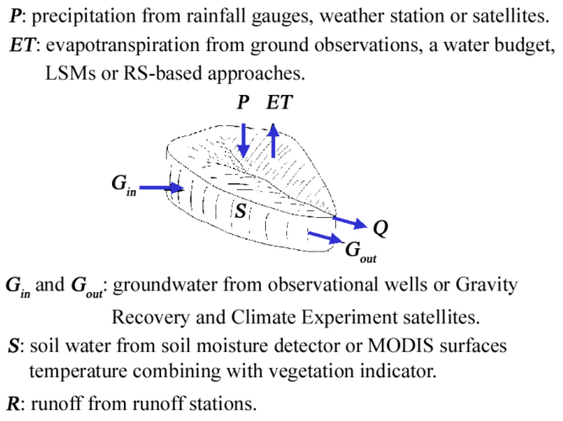
A wide range of global and regional ET products have been developed in recent decades for monitoring water use and assisting in planning management. They can be broadly classified into three categories: remote sensing (RS)-based ET products using vegetation index-based data or land surface temperature (LST) (e.g., the Moderate Resolution Imaging Spectroradiometer (MODIS) ET, Advanced Very High Resolution Radiometer (AVHRR) ET, Priestly-Taylor Jet Propulsion Laboratory (PT-JPL) ET and Global Land Evaporation Amsterdam Model (GLEAM) ET), ET output from land surface models (LSMs) (e.g., Global Land Data Assimilation System (GLDAS) ET, Modern-Era Retrospective analysis for Research and Applications (MERRA) ET and European Centre for Medium-Range Weather Forecasts Re-analysis (ERA)-interim ET), and ET from a water budget with measured precipitation, runoff and total water storage change (e.g., TerraClimate ET and Gravity Recovery and Climate Experiment (GRACE)-inferred ET) [5,11,12]. These ET products have been used to a varying degree for irrigation water management [8], vegetation productivity estimation [9,10], calibration and optimization of hydrological models and prediction of runoff in the ungauged basins [13,14], and water management modes and water rights regimes [2,15,16]. However, these different ET products are of different spatial-temporal scales, and differ in accuracy or uncertainty [11,17,18].
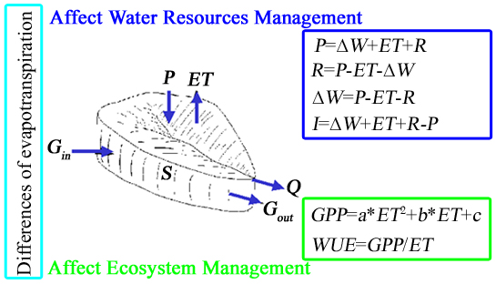
As ET is the largest water-use component in the catchment water balance in arid and semi-arid regions, any variation of ET will cause corresponding errors in the estimation of runoff and soil water storage, thus also large errors in the determination of water demand of irrigated agriculture and in the estimation of productivity of water use in an ecosystem [19,20]. To date, most hydrologic studies, as well as river basin management proposals, have tended to focus on supply elements e.g., precipitation, snow, runoff, water storage soil moisture and groundwater, but have largely ignored the demand side (e.g., ET) (Figure 1) [5]. This is mainly because of insufficient knowledge of ET at local to global scales. The ground observations for ET (eddy covariance towers, Bowen ratio systems, and weighing lysimeters) are poorly covered in many regions, furthermore there are uncertainties about the ET from a water budget perspective which accumulate from errors in other hydrological components, and uncertainties of the ET from land surface models and RS-based approaches due to differences in the structures, resolutions, and inputs of the models and approaches. However, the range of these errors caused by the variations of ET products is not yet clear. Without such knowledge, our capacity for accurate water resource management, economic development and sustainable ecosystems would be seriously compromised.
This paper aims to analyse the chain effects of variations of several widely used ET products on water resource and ecosystem management in which the Murrumbidgee River catchment (hereafter MRC) in Australia, a semi-arid and arid catchment with the intensified agriculture and declining ecosystems, is taken as a case study area. The water balance in the MRC obtained from the Australian Water Availability Project (AWAP) datasets from 2001–2016 will be used as the “reference” and to compare the performance differences of four global representative ET products selected from dozens of products: a RS-based ET product from MODIS, a LSMs-based ET product from GLDAS, a water budget-based ET product from TerraClimate and the ET product developed by the Australian indigenous research institute, the Commonwealth Scientific and Industrial Research Organisation (CSIRO), and their effects on the other water balance components, irrigation, and gross primary productivity (GPP) and water-use efficiency of forest and grassland are analysed.
2. Methods and Data
2.1. Study Area
The Murray–Darling Basin (hereafter MDB) is the most productive agricultural area in Australia and a globally recognized epitome of successful water management. It covers around 14% of Australia’s land, but produces about 40% of Australia’s gross value of agricultural production. As one of the most important catchments in the MDB, the MRC has an area of 84,000 square kilometers and accounts for about 7.9% of the MDB (Figure 2). It encompasses all of the Australian Capital Territory. The Murrumbidgee River rises in the Snowy Mountains and flows 1690 km from east to west. The average annual runoff is about 37.84 × 10⁸ m3. The highest precipitation occurs in the eastern mountains of the catchment and averages 1500 mm yr−1, while the average annual rainfall in the lower catchment is about a fifth of this figure. The annual potential ET ranges from 1250 mm to 1500 mm. Most of the precipitation losses are in the form of ET and account for up to 90%.
The MRC was opened to settlement in the 1830s and soon became an important farming area, and now its irrigated area accounts for about 15% of the total in the MDB, especially the irrigated rice area which is up to about two third of the total rice area in the MDB according to the statistical data from Australian Bureau of Agricultural and Resource Economics and Sciences (ABARE). In the MRC, agricultural land, grassland, and forest are the main land cover types, which accounts for about 60%, 15%, and 20%, respectively [21]. The Murrumbidgee River is one of the most regulated rivers in Australia on which there are 26 water storage structures. Irrigation for agriculture is the greatest user of water in the MRC, and the total volume of irrigation entitlements is approximately 28.0 × 10⁸ m3, which accounts for 74.0% of the average annual runoff [22]. However, with the development of the farming practices, there is increasing deterioration of river health, thus, protection of the environment is on the political agenda, along with a commitment not only to return water to rivers to nurse them back to health, but also to help agricultural industries rise up to the challenge of a drier climate [23]. In such a catchment, precise and reliable water resources management is extremely important for agricultural development and ecosystem management.
2.2. Data Sources and Processing
The AWAP datasets concern the terrestrial water balance across continental Australia and are developed by the Australian Water Availability Project (AWAP, http://www.csiro.au/awap) Team and the CSIRO Marine and Atmospheric Research using the WaterDyn model. They include a long-term historical monthly time series (data set “Run 26m”, 1900 to 2017) of the conventional water balance components at a spatial resolution of 0.05° [24]. These datasets have been widely used in research on water resource management in Australia and can be viewed as referenced or observational data to evaluate the other types of water balance components [25]. The water balance components (in mm mon−1) of the MRC from 2001 to 2016, including precipitation, ET, runoff, and soil water storage changes were obtained from these datasets.
The four other ET products selected for comparative analysis include ET from CSIRO, GLDAS, MODIS, and TerraClimate. The CSIRO ET is a monthly global ET product developed by the CSIRO [26]. The estimates are computed through the observation-driven Penman–Monteith–Leuning (PML) model. The GLDAS ET is the GLDAS-2.1 ET product, which is one of two components of the GLDAS Version 2 (GLDAS-2) dataset and is developed with the advanced land surface modeling and data assimilation techniques utilising satellite and ground-based observational data products [27]. The MODIS ET is the MOD16A2 Version 6 Evapotranspiration/Latent Heat Flux product and is an 8-day composite product produced at 500-metrepixel resolution [28]. The algorithm used for the MOD16 data product collection is based on the logic of the Penman–Monteith equation, which includes inputs of daily meteorological reanalysis data along with MODIS remotely sensed data products such as vegetation property dynamics, albedo, and land cover. The TerraClimate ET is the actual evapotranspiration of TerraClimate dataset and is derived using a one-dimensional soil water balance model [29]. TerraClimate is a dataset of monthly climate and climatic water balance for global terrestrial surfaces. It uses climatically aided interpolation, combining high-spatial resolution climatological normals from the WorldClim dataset, with coarser spatial resolution of 2.5°.
Other data used in this study include irrigation information, ecosystem data, and land cover data. The irrigation information was obtained from farm survey reports from ABARE, which is the only national farm survey information source in Australia. As one of the most important indicators of ecosystem function and closely related to water use, the GPP was selected for ecosystem assessment. The GPP data is the MOD17A3 V055 product, which provides information about annual GPP at 1 km pixel resolution [30]. In addition, we used the current release of the second version of the Dynamic Land Cover Dataset (DLCDv2.1) as a basis for water balance analyses [21]. The land cover classification scheme conforms to the 2007 International Standards Organisation (ISO) land cover standard (19144-2). In this dataset Australian land covers are clustered into 22 classes, ranging from cultivated and managed land cover to natural land cover. The data presents land cover information for every 250 m by 250 m area of the country at a two-year interval. In accord with our research aim in this study, we combined these 22 land cover types into 7 types: bare surface, water bodies/wet land, irrigated agriculture, rain-fed agriculture, grassland, forest, and urban area. Then, we uniformly resampled and adjusted resolution of the spatial data (except AWAP data set and CSIRO ET) to 500 m and projection and temporal resolutions (annual and monthly) to make the data products comparable using the Google Earth Engine (GEE). Manipulation of the AWAP data set and CSIRO ET, and reclassification and combination of land cover data were conducted in the ArcGIS platform. We made the analysis based on the land cover types in monthly and annual scales respectively using SPSS and Microsoft Excel software.
All data used in this study including the water balances components from AWAP, the ET products from CSIRO, GLDAS, MODIS, and TerraClimate, irrigation information, land cover, and GPP are summarized in Table 1.
2.3. Comparison among These Five Evapotranspiration (ET) Products
The variations of ET among the products were quantified by comparing the four ET products (comparison value) with the AWAP ET component (reference value). The percent bias (PBIAS) and mean absolute error (MAE) were used [31] to assess the difference between the reference and comparison ET values. PBIAS measures the average tendency of comparison values. Positive values show overestimation and negative values indicate underestimation; low-magnitude values of PBIAS are preferred and the optimal value is 0. MAE means the average value of the absolute errors between the reference and comparison ET values and can better reflect the actual level of the comparison value error. The smaller the MAE, the better the comparison value. They are calculated as follows:
The root mean square error (RMSE) and root mean square error observation standard deviation ratio (RSR) were then used to derive statistical goodness of fit of the ET comparison values and to evaluate the performance of the data product against reference values. RMSE is very sensitive to the large errors in a group of data. RSR is used to standardise RMSE and integrate the advantages of error statistics, and RSR ranges from 0 to 1. They are computed using the following equations:
Following on, the coefficient of determination (R2) value was computed to evaluate the linear relationship between reference and comparison ET data. Along with R2, we also reported slope and intercept values to provide useful information of the degree of bias at higher ET and intercept for the magnitude of bias affecting lower comparison ET. R2 ranges from 0 to 1, and this represents the proportion of the total variance in the reference data that can be explained, with higher R2 values indicating better performance.
Finally, the Nash–Sutcliffe efficiency (NSE) [32] was used to measure how well comparison values represent the reference data, relative to a prediction made by using the average reference value. It is a more stringent measure than R2. NSE ranges from −∞ to 1, with NSE = 1 being the optimal value. NSE is calculated as:
where Qisim is the comparison ET (other four ET products), and Qiobs is the reference ET (AWAP ET) at time step i, respectively, whereas Qavgobs and Qavgsim are the average reference and comparison ET values, and n is the total number of data, and subscript i represents the time step (month or year).
2.4. The Effects of ET Variations on the Runoff and Water Storage Changes
The catchment water balance approach was used to analyse the effects of value differences in these ET products on the runoff and water storage changes. The water balance approach, routinely used for estimating mean annual ET, is based on the catchment water budget [33]. For a given watershed, the instantaneous equation of the water mass balance is:
where P, ΔW, ET, and R are precipitation, water mass storage changes, evapotranspiration, and runoff respectively. These terms are generally expressed in terms of water mass (mm of equivalent water height) per day. There are many transformations for the Equation (7) for different purposes and based on different available data.
To assess the effects of ET variations on runoff, other terms of the equations were set at AWAP levels with ET values from the other four products were used respectively, and the equation can be transferred into the following:
To assess the impacts of ET variations on water storage changes, other terms of the equations were set at AWAP levels with ET values from the four products were used respectively, and the equation can be transferred into the following:
2.5. The Chain Effects of ET Variations on Irrigation
For water catchments with intensive irrigation, irrigation water (I) as an external source should be added to Equation (7). Then the equation of water mass balance is given as:
Because the detailed groundwater observational data is lacking and the main irrigation water resources in this catchment is surface water, and the recharge to the groundwater through infiltration of irrigation water is very small according to data drawn from ABARE’s farm survey reports, two assumptions were made: only when the sum of ET and R was more than P, I was calculated by dividing the P from the sum of the ET and R, and ΔW was viewed as 0 in Equation (12); and when the sum of the ET and R was less than or equal to P, there was no irrigation, and ΔW was the difference between P and the sum of the ET and R in Equation (13).
2.6. The Chain Effects of ET Variations on Productivity and Water-Use Efficiency of Ecosystems
The large water consumption sectors in the ecological systems in the MRC include the grasslands and forest. GPP, the most important indicator related to both the water cycle and carbon cycle, is used to measure the effects of ET variations on terrestrial ecosystems because of the linear relationship between GPP and ET at a regional scale [34]. In the MDB, it was modified from a linear relationship to a quadratic relationship [10]. The function between annual GPP and ET is given in Equation (14).
where ET is the total ET per unit area in mm yr−1, GPP is the total GPP in g C m−2 yr−1.
The water-use efficiency, reflecting the water stress under the different water conditions of the ecosystem, is the ratio of the GPP to the ET, and can be calculated as:
where WUE is the water use efficiency in g C m−2 per mm water or kg C m−3 H2O. The parameters a, b, and c were determined with the observed GPP from 2001 to 2014 and the varying ET products.
3. Results
3.1. ET Comparison among the Five ET Products
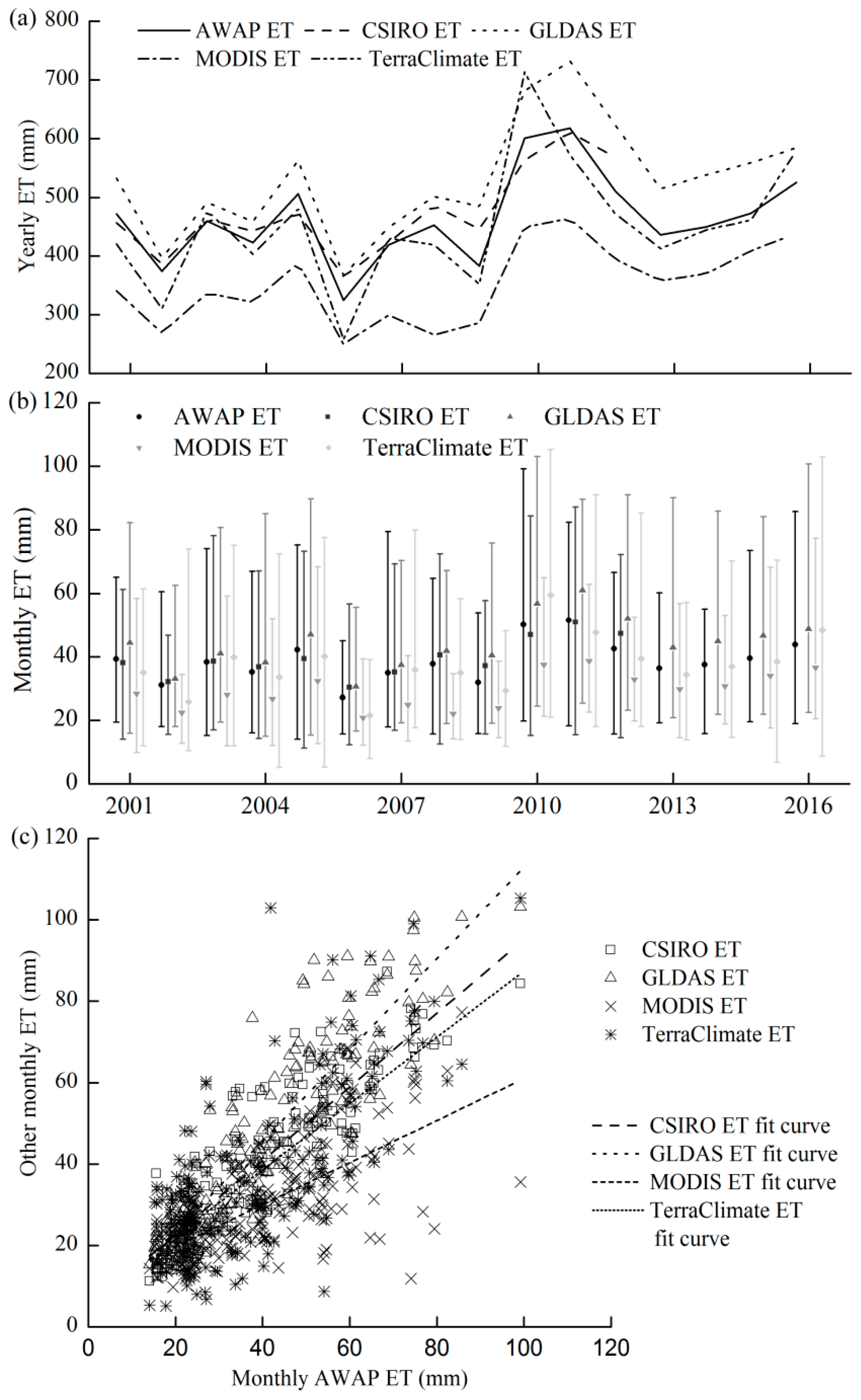
The fluctuations of the annual ET are obvious, where the minimum values appeared in 2006, and the maximum values appeared in 2011 (except for the TerraClimate ET) (Figure 3a). Although the change trends of all ET products are similar, the differences between their extreme annual values are large. For example, the largest is up to 455.3 mm for the TerraClimate ET while the minimal is only 214.7 mm for the MODIS ET. The minimum and maximum annual ET values are 324.7 mm and 617.8 mm (AWAP); 364.3 mm and 611.2 mm (CSIRO); 366.7 mm and 732.5 mm (GLDAS); 249.6 mm and 464.3 mm (MODIS); and 257.8 mm and 713.1 mm (TerraClimate), respectively. Their ratios of the maximum to the minimum annual ET values are 1.9, 1.7, 2.0, 1.9 and 2.8, respectively. Moreover, there are differences among their average values (Table 2). The average value of GLDAS ET is 14% more than the AWAP ET, while MODIS ET is 24% less than the AWAP ET. The CSIRO ET and TerraClimate ET are very close to the AWAP ET. Their RMSE and MAE were smaller as RSR’s values were around 0.5, and the PBIAS values were close to 0.
The mean, maximum, and minimum values of the monthly ET each year are shown in Figure 3b, and the variations of the mean monthly ET are the same as the yearly ET, but the changes of maximum and minimum values are very different. Compared with the AWAP ET, both the maximum and minimum values of GLDAS ET are larger, while the maximum values of MODIS ET are less, and its minimum values are less before 2010 and then almost the same since 2010. For the CSIRO and TerraClimate ET, their maximum values are similar to the AWAP ET, but the minimum values are less than the AWAP ET, and the TerraClimate ET is more obvious. The range of the monthly values are from 14.0 mm to 99.2 mm (AWAP), 11.2 mm to 87.2 mm (CSIRO), 15.0 mm to 103.1 mm (GLDAS), 9.8 mm to 77.3 mm (MODIS), and 5.1 mm to 105.3 mm (TerraClimate). Their ratios of the maximum to the minimum monthly ET values are up to 7.1, 7.8, 6.9, 7.9, and 20.6, respectively. Figure 3c shows the scatter diagram between the monthly AWAP ET with the other ET products from 2001 to 2016, and the performances of the fitting relationship between the GLDAS ET and CSIRO ET and AWAP ET are better than the other two ET products, which can be reflected by the slopes of fitting lines around 1 and correlation coefficients of more than 0.75 (Table 2). According to the other evaluation indicators, the CSIRO ET is the best among the four ET products, because its NSE is the largest, while the RMSE, RSR, and MAE are the smallest.
3.2. The Effects of ET Variations on Estimation of Runoff and Water Storage Changes
3.2.1. The Water Balance in the Murrumbidgee River Catchment (MRC) Using Australian Water Availability Project (AWAP) Datasets
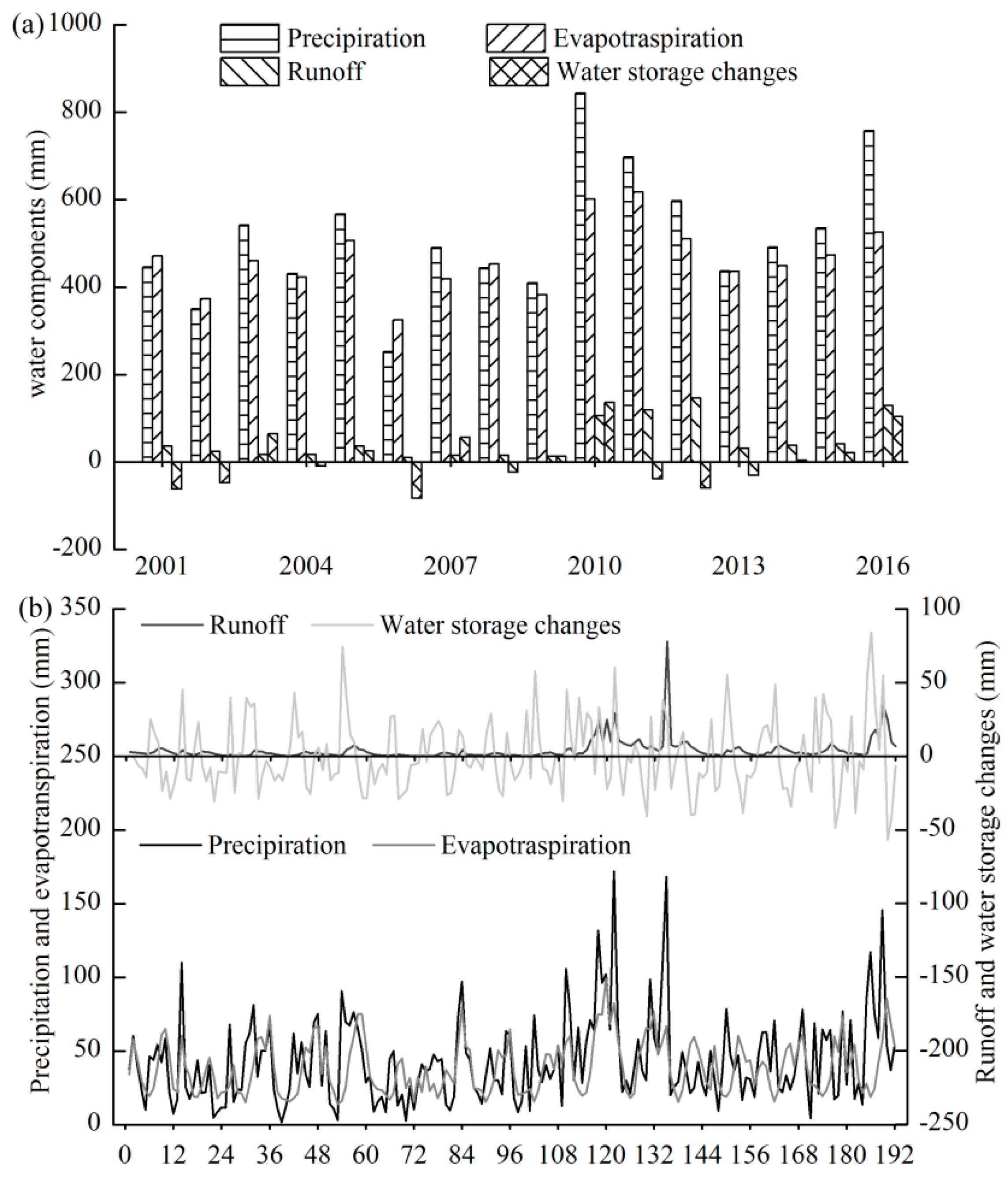
Figure 4 shows the annual and monthly water balance in the MRC using AWAP datasets. The mean annual precipitation, ET, runoff, and water storage changes are 518.0 mm, 464.1 mm, 49.5 mm, and 4.4 mm, respectively. The years of 2002, 2006, and 2009 were the dry years, while 2010, 2011, and 2016 were wet years. In most years, the precipitation is largely lost by ET, and in some years even the latter is larger than the former due to relatively less precipitation and consumption of the soil water. The runoff is low except in the very wet years, and the water storage is in a deficit condition. This situation was most serious in 2006.
The precipitation and ET in the MRC are concentrated in the period from December to February. The runoff only appeared in heavy rain years, for example, in 2010, 2011, and 2016. In some months, ET is more than precipitation, which leads to water storage changes: a recharge in heavy rain years and a deficit in drought years.
3.2.2. The Effects of ET Variations on Runoff Estimation
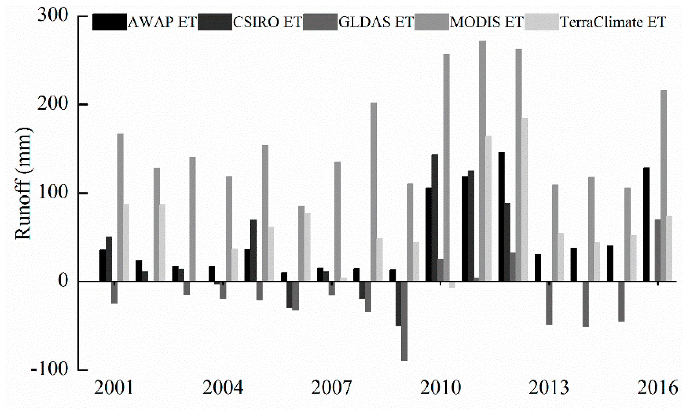
Figure 5 shows the annual runoff estimated using the four ET products combining the AWAP precipitation and water storage data. Compared with the AWAP runoff, the runoff estimated using the MODIS ET is much larger, while the runoff estimated using the TerraClimate ET is larger in some years and less in other years and even is negative in 2010. The runoff estimated using the GLDAS ET is much less than the AWAP runoff and even becomes negative. The runoff estimated using the CSIRO ET is complex, because it is larger or less than the AWAP runoff in some years but is negative in other years. The mean annual runoff estimated using the ET products from AWAP, CSIRO, GLDAS, MODIS, and TerraClimate are 49.5 mm, 34.4 mm, −16.3 mm, 161.3 mm, and 63.2 mm respectively. Application of the CRISO and GLADS ET products results in the underestimation of runoff, on the contrary, the MODIS and TerraClimate ET products result in the overestimation of runoff. The runoff estimated using the GLDAS ET is negative, while the runoff estimated using the MODIS ET is more than triple that of the AWAP runoff.
3.2.3. The Effects of ET Variations on Water Storage Estimation
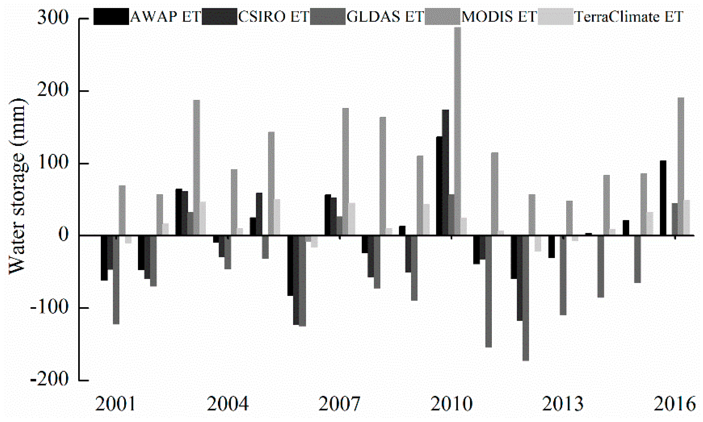
Figure 6 shows the annual water storage estimations using the four ET products combining the AWAP precipitation and runoff data. Compared with the AWAP water storage, the water storage estimated using the MODIS ET is much larger and positive except for the negative value in 2006 which was an extremely dry year, while the water storage estimated using the TerraClimate ET is larger in most years and less in a few years. The water storage estimated using the GLDAS ET is much less than the AWAP water storage and was negative in most years except in 2003, 2007, 2010, and 2016. The water storage estimated using the CSIRO ET is similar to the AWAP’s estimations, but the former was negative while the latter was positive in 2009. The mean annual water storage estimated using the ET products from AWAP, CSIRO, GLDAS, MODIS, and TerraClimate are 4.4 mm, −14.1 mm, −61.5 mm, 116.1 mm, and 18.1 mm, respectively. The CSIRO and GLDAS ET products result in the underestimation of water storage, which indicates that the water storage is in deficit. By contrast, the MODIS and TerraClimate ET products result in the overestimation of water storage. The water storage estimated using the MODIS ET is even up to 110 mm and more than the AWAP water storage.
3.3. The Effects of ET Variations on Irrigation Estimation
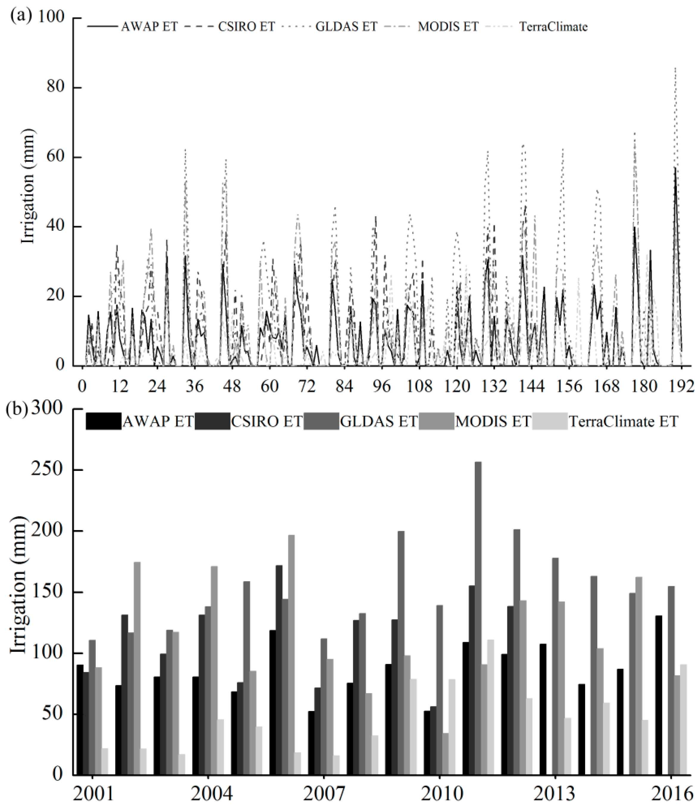
Figure 7 shows the monthly and annual irrigation water estimated using the five ET products combining the AWAP precipitation and runoff data in irrigated area in the MRC. There are significant differences between them, and the average values of annual irrigation water estimated using the AWAP, CSIRO, GLDAS, MODIS, and TerraClimate ET products are 87.0 mm, 114.2 mm, 154.6 mm, 115.7 mm, and 49.1 mm, respectively. The maximal one, estimated using MODIS ET, is more than three times of the minimal one estimated using TerraClimate ET. Compared with the annual irrigation water estimated using the AWAP, the CSIRO’s are larger except in 2001, the GLDAS’s are larger, the MODIS’s are larger in most years, and the TerraClimate’s are less except in 2010 and 2011. Although the irrigation water estimated using CSIRO and MODIS ET are close, they are different both over monthly and annual scales. The maximum values of the annual irrigation water using the AWAP, CSIRO, and MODIS ET products appeared in 2006 and were 118.8 mm, 171.8 mm, and 196.6 mm, respectively, while the maximum values using the GLDAS and TerraClimate ET products appeared in 2011 and were 256.5 mm and 110.9 mm, respectively.
3.4. The Effects of ET Variations on the Gross Primary Productivity (GPP) and Water-Use Efficiency of the Grassland and Forest
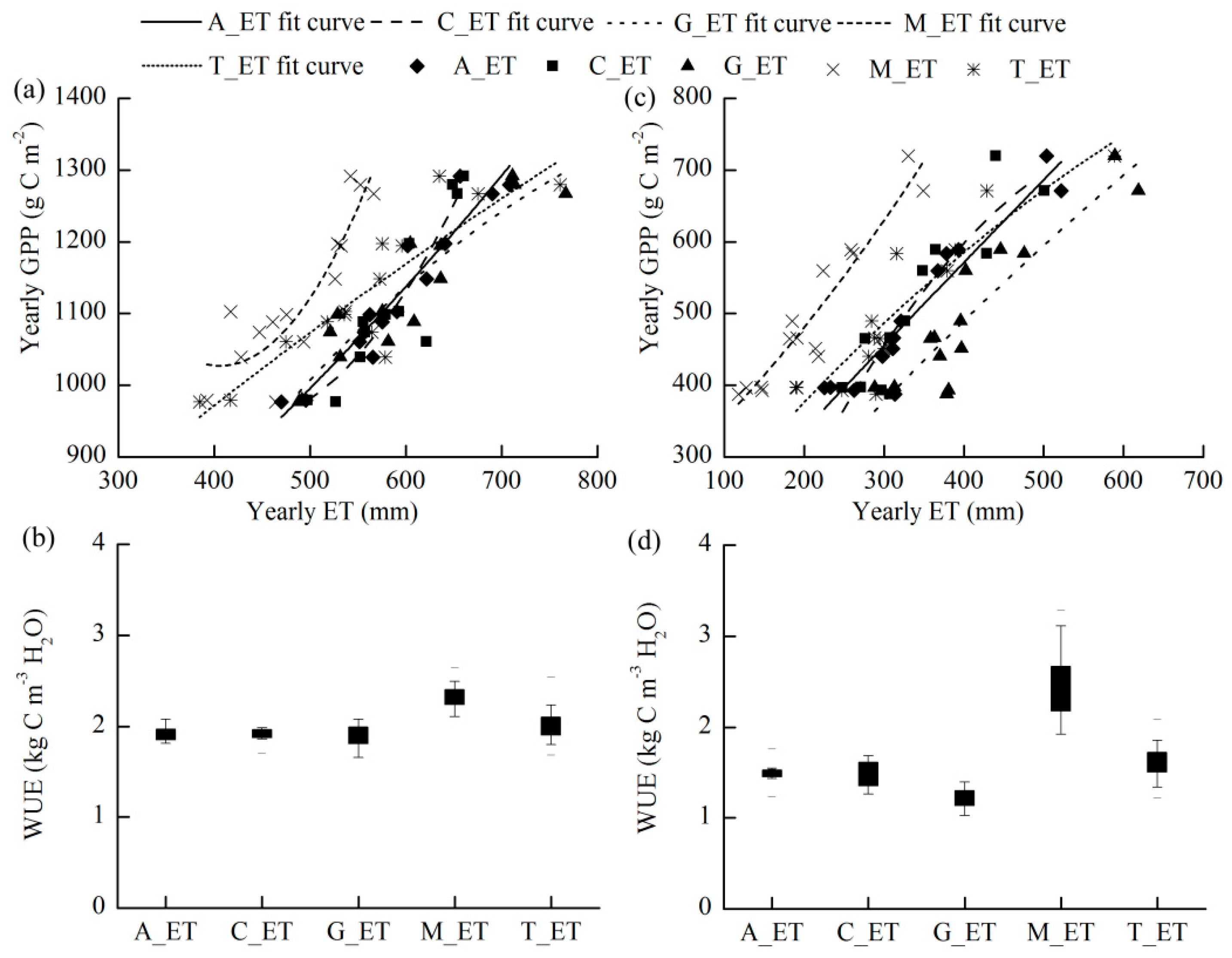
The annual GPPs range is from 976.8 g C m−2 to 1279.5 g C m−2 for forest and 397.0 g C m−2 to 719.6 g C m−2 for grassland, and the annual ETs range is from 384.8 mm to 766.6 mm for forest and 118.0 to 618.8 mm for grassland (Figure 8a,c). The points representing different ET products overlap each other except for the MODIS ET for forest (Figure 8a), which indicates the ET products are close. However, the points representing GLDAS ET and MODIS ET are located at the left and right respectively, and the other three ET products are located in the middle and have some overlap for grassland, which reflects the obvious differences among the ET products (Figure 8c). There are significant quadratic relationships between the yearly GPP and all ET for forest and grassland, but the quadratic functions are different from each other (Figure 8a,c). For forest, the mean water use efficiency estimated using AWAP, CSIRO, GLDAS, and TerraClimate ET are close and about 1.9 kg C m−3 H2O, while the water-use efficiency estimated using MODIS ET is up to 2.3 kg C m−3 H2O (Figure 8b). For grassland, the mean water use efficiency estimated using AWAP, CSIRO, GLDAS, MODIS, and TerraClimate ET are 1.5 kg C m−3 H2O, 1.5 kg C m−3 H2O, 1.2 kg C m−3 H2O, 2.4 kg C m−3 H2O, and 1.6 kg C m−3 H2O (Figure 8d). The ranges of the annual water-use efficiency estimated using AWAP, CSIRO, MODIS, and TerraClimate ET for forest are less than those for grassland, and the ranges using GLDAS ET are the same.
4. Discussion
4.1. The ET Variations among the Five Products
The results show that there are obvious differences in the annual and monthly ET values among these five ET products. The possible reasons for these ET variations could be explained as follows.
(1) Different estimation approach. GLDAS ET is the simulation from a land surface model which is upscaling of space- and ground-based observations with data assimilation techniques [27]. MODIS ET is the terrestrial ET based on the logic of the Penman–Monteith equation, which includes inputs of daily meteorological reanalysis data from the Global Modelling and Assimilation Office of NASA along with MODIS remotely sensed data products [28]. TerraClimate ET is developed using a water balance model that incorporates reference evapotranspiration, precipitation, temperature, and interpolated plant extractable soil water capacity, while the AWAP ET is also developed using a water balance model, and their results are close except that there is a larger difference in grassland. This is because the TerraClimate ET uses a simplified one-dimensional Thornthwaite–Mather water balance model while AWAP employs a two-layer model to simulate the changes in the shallow (thickness 0–0.7 m) and deep (0.2–1.5 m) soil layers, and the latter can depict the loss of the deep soil water [24,29]. Compared with the above three ET products, the CSIRO ET is similar to the AWAP ET, which is because they share many basic input data in this catchment [24,26]. CSIRO ET uses an observation-driven Penman–Monteith–Leuning (PML) model, supported with meteorological forcing data and along with satellite derived vegetation forcing data, land cover data, emissivity, and albedo. This is similar with the MODIS ET using the Penman–Monteith method and remotely sensed data, but their results are different in the interannual change, annual change, average value of the ET, and the ET of each land use type. This might be explained as the input datasets applied in CSIRO ET better represent the characteristics of Australian territory [26,28].
(2) Different inputs. There are obvious differences among inputs, such as meteorological forcing data, vegetation forcing data, and land surface data. For example, the precipitation, a key factor determining water availability and a basic component of the hydrological cycle, is different from each other in these ET products. GLDAS ET uses the space- and ground-based precipitation observations with data assimilation techniques, MODIS ET uses the daily meteorological reanalysis data, while AWAP ET uses a gridded daily rainfall dataset, which can directly influence the ET [24,27,28].
(3) Different spatial-temporal scales. The spatial scale mismatch between finer vegetation data and coarser meteorological forcing could result in large variations in ET products [11,35]. The spatial resolutions of these five ET products are different from each other and range from 500 m of MODIS ET to 2.5° of the TerraClimate ET. Generalisation of surface features (such as land use/cover and terrain) leads to the decreases of the resolution, thus the loss of details of surface features. The temporal resolutions of these five ET products vary from 3 h to one month, which could result in the representation of different meteorological processes and vegetation physiological processes in these ET products [14].
(4) The different expression of dynamics in vegetation index-based data could also cause differences among ET products. Some ET estimation methods, based on remotely sensed data like MODIS, can timely reflect the vegetation changes, but others cannot. If the vegetation growth process cannot be truly expressed, the evapotranspiration of vegetation, as well as its photosynthesis and other related hydrological processes (such as canopy interception and infiltration) will be affected [14].
4.2. The Effects of the Variations among the ET Products on Water Resources Management
ET is a significant climate variable that uniquely links the water cycle. It can help understand both sides of the water supply-demand equation [5,36]. The model calibration, using ET products combined with gaged runoff data, have effectively improved the performances of the hydrological models; moreover, ET products are also attractively used to estimate the runoff in the ungauged basins [5,13,14]. Thus, the value variations of ET could have a large influence on the other water balance components. Compared with the gaged runoff data and the condition of the total water storage changes estimated with the GRACE satellites from 2002 to 2014 [37], the runoff and water storage change in the MRC provided by the AWAP are reasonable respectively. The results in this study show the obvious influences of different ET products on the estimation of runoff and water storage undoubtedly creates a challenge for the calibration of hydrological models with such large variations of water balance components [13,14,19]. More importantly, such inaccurate information would seriously influence the precision and reliability of the decision-making on regional water resources allocation and regulation, which may artificially aggravate the unbalance of water allocation between different reaches in catchments, and between human resource use and ecosystem protection. In addition, such large variations of ET cast a shadow over the objective assessment of the effects of land use and cover change and climate change on basin water cycles, which are attracting increasing global attention [38,39].
As the predominant variable for water management in agricultural food production, the atmospheric demand for ET is a reference to irrigation [40,41]. In the MRC, the uncertainty of water allocation and low water availability were the main impediments to irrigated farms including dairy, broadacre and horticultural industries [42]. It was found in this study that the estimations of annual irrigation with these five ET products range from 49.1 mm using TerraClimate ET to 154.6 mm using GLDAS ET. Such a large range of estimated irrigation could lead to over-irrigation with water loss via infiltration of groundwater or it could result in unnecessarily returning water to rivers for environmental protection at the expense of necessary irrigation, resulting in lower crop yields due to crops suffering the effects of insufficient water, especially during the growth stage of the crop.
4.3. The Influences of the Variations among the ET Products on Ecosystem Management
The latest research found that the global carbon sink anomaly was driven by growth of semi-arid vegetation in the Southern Hemisphere, with almost 60 per cent of carbon uptake attributed to Australian ecosystems. This finding suggested that the higher turnover rates of carbon pools in semi-arid biomes were an increasingly important driver of inter-annual variability of global carbon cycle [43]. ET is the loss of water when mitigating vegetation stress responses and becomes the indicator of ecosystem function and health, such as productivity and carbon dioxide regulation [5]. In this study, it was found that there are less differences between the five ET products when applied to forest than when applied to grassland, thus there are also different relationships between GPP and different ET products for forest and grassland. However, all of their relationships are in significantly quadratic correlations. This means that we likely think that it is credible to predict the GPP using any of these relationships and the related ET products, which will probably result in different GPP estimations with different ET products. Water-use efficiency reflects the water stress of forest and grassland and therefore is a very important indicator of ecosystem health. It is found in this study that the mean water use efficiency of the forest using AWAP, CSIRO, GLDAS, and TerraClimate ET are about 1.9 kg C m−3 H2O and are all greater than the grasslands, from the 1.2 kg C m−3 H2O of GLDAS to 1.6 kg C m−3 H2O of TerraClimate ET. However, the water-use efficiency estimated using MODIS ET is 2.3 kg C m−3 H2O for forest, while grassland’s is up to 2.4 kg C m−3 H2O showing greater water use efficiency than forest. These values are reasonable according to the previous findings reporting C3 species range between 1.4 and 3.6 kg C m−3 H2O [44], but the large range of GPP estimation functions and WUE among the five ET products could influence the precision in the assessment of the ecosystem function (e.g., carbon dioxide regulation) and how terrestrial ecosystems respond to environmental changes (e.g., a drier climate). Furthermore, the value variations of ET can seriously affect the allocation of environmental flows, especially in arid regions where the water resource is even scarcer. It also can affect the migration of water, salt and nutrient in the basin water quality modeling, then lead to the inaccurate prediction and evaluation of salinization, eutrophication, and ecological degradation.
4.4. Limitations
It should be noted that there are limitations in the methods and data in this study. We used the conventional water balance equation with fewer data requirements to assess the effects of ET variations on each water balance component. It should be known that the physical hydrological models reflecting the complex hydrological processes of the catchment could have more precise results. Meanwhile, we estimated the irrigation water amount according to the ET without consideration of the influence of different agricultural management practices, especially with the assumption of the unchanged water mass storage under irrigation practices. Nevertheless, as the focus of this study was to compare the effects of different ET products on runoff, water storage, and irrigation water amount, this simplified method was good enough to address the research questions in this study.
5. Conclusions
In this study, we provided quantitative effects of the value variations of several widely used ET products (AWAP, CSIRO, GLDAS, MODIS, and TerraClimate) on water resources management and ecosystem assessment using a water balance equation and its transformations, the relationships between GPP, WUE and ET. There are obvious differences of ET value among the five ET products in the MRC at annual and monthly scales. This leads to huge differences in the estimations of annual runoff (−16.3 to 161.3 mm) and annual water storage (−61.5 to 116.1 mm) and also for the annual irrigation water per area requirements ranging from 49.1 mm to 154.6 mm. The ET products for forest are relatively consistent among each other, but those for grassland present a large varying range. There are different productivity predictions of the ecosystem with the same water use based on the relationships between the annual GPP and varying ET for both forest and grassland, however, the forest has a better capacity of dealing with water stress than the grassland according to the values and the change amplitudes of their WUE. The effects of the variations among the ET products on water resources and ecosystem management are remarkable and need to attract more attention.
Author Contributions
Y.W. and Q.F. designed the case study. Z.L. and Y.Z. processed the data. Z.L. and Y.W. wrote the draft. Y.Z. and J.X. revised the draft. All of the authors contributed to the discussion of the results.
Funding
This work was funded by the National Natural Science Foundation of China (Project No: 41601036, 41571031), "Light of West China" Program of CAS, the International Postdoctoral Exchange Fellowship Program, the Australian Research Council (Project No: FT130100274), and the Strategic Priority Research Program of the Chinese Academy of Sciences (Project No: Y82CG11001).
Acknowledgments
The data are available from the corresponding data sites and providers listed in Table 1. We thank the two referees as well as the editors for providing valuable comments.
Conflicts of Interest
The authors declare no conflict of interest.
References
- Elimelech, M.; Phillip, W.A. The future of seawater desalination: Energy, technology, and the environment. Science 2011, 333, 712–717. [Google Scholar] [CrossRef] [PubMed]
- Jia, Z.; Liu, S.; Xu, Z.; Chen, Y.; Zhu, M. Validation of remotely sensed evapotranspiration over the Hai River Basin, China. J. Geophys. Res. Atmos. 2012, 117, 1–21. [Google Scholar] [CrossRef]
- Vörösmarty, C.J.; McIntyre, P.B.; Gessner, M.O.; Dudgeon, D.; Prusevich, A.; Green, P.; Glidden, S.; Bunn, S.E.; Sullivan, C.A.; Liermann, C.R. Global threats to human water security and river biodiversity. Nature 2010, 467, 555. [Google Scholar] [CrossRef]
- Bakker, K. Water security: Research challenges and opportunities. Science 2012, 337, 914–915. [Google Scholar] [CrossRef]
- Fisher, J.B.; Melton, F.; Middleton, E.; Hain, C.; Anderson, M.; Allen, R.; McCabe, M.F.; Hook, S.; Baldocchi, D.; Townsend, P.A. The future of evapotranspiration: Global requirements for ecosystem functioning, carbon and climate feedbacks, agricultural management, and water resources. Water Resour. Res. 2017, 53, 2618–2626. [Google Scholar] [CrossRef] [Green Version]
- Owen, C.R. Water budget and flow patterns in an urban wetland. J. Hydrol. 1995, 169, 171–187. [Google Scholar] [CrossRef]
- Fahle, M.; Dietrich, O. Estimation of evapotranspiration using diurnal groundwater level fluctuations: Comparison of different approaches with groundwater lysimeter data. Water Resour. Res. 2014, 50, 273–286. [Google Scholar] [CrossRef] [Green Version]
- Or, D.; Hanks, R. Spatial and temporal soil water estimation considering soil variability and evapotranspiration uncertainty. Water Resour. Res. 1992, 28, 803–814. [Google Scholar] [CrossRef]
- Fatichi, S.; Ivanov, V.Y. Interannual variability of evapotranspiration and vegetation productivity. Water Resour. Res. 2014, 50, 3275–3294. [Google Scholar] [CrossRef] [Green Version]
- Zhou, S.; Huang, Y.; Wei, Y.; Wang, G. Socio-hydrological water balance for water allocation between human and environmental purposes in catchments. Hydrol. Earth Syst. Sci. 2015, 19, 3715–3726. [Google Scholar] [CrossRef] [Green Version]
- Long, D.; Longuevergne, L.; Scanlon, B.R. Uncertainty in evapotranspiration from land surface modeling, remote sensing, and GRACE satellites. Water Resour. Res. 2014, 50, 1131–1151. [Google Scholar] [CrossRef] [Green Version]
- Drexler, J.Z.; Snyder, R.L.; Spano, D.; Paw U, K.T. A review of models and micrometeorological methods used to estimate wetland evapotranspiration. Hydrol. Process. 2004, 18, 2071–2101. [Google Scholar] [CrossRef]
- Rajib, A.; Evenson, G.R.; Golden, H.E.; Lane, C.R. Hydrologic model predictability improves with spatially explicit calibration using remotely sensed evapotranspiration and biophysical parameters. J. Hydrol. 2018, 567, 668–683. [Google Scholar] [CrossRef]
- Rajib, A.; Merwade, V.; Yu, Z. Rationale and efficacy of assimilating remotely sensed potential evapotranspiration for reduced uncertainty of hydrologic models. Water Resour. Res. 2018, 54, 4615–4637. [Google Scholar] [CrossRef]
- Zhong, Y. Analysis of water rights system based on ET. Water Resour. Dev. Res. 2007, 2, 14–16. [Google Scholar]
- Tang, W.; Zhong, Y.; Wu, D.; Deng, L. Analysis of water resource management mode based on ET. China Rural Water Hydropow. 2007, 10, 8–10. [Google Scholar]
- Sörensson, A.A.; Ruscica, R.C. Intercomparison and uncertainty assessment of nine evapotranspiration estimates over South America. Water Resour. Res. 2018, 54, 2891–2908. [Google Scholar] [CrossRef]
- Allen, R.G.; Pereira, L.S.; Howell, T.A.; Jensen, M.E. Evapotranspiration information reporting: I. Factors governing measurement accuracy. Agric. Water Manag. 2011, 98, 899–920. [Google Scholar] [CrossRef]
- Lu, Z.; Zou, S.; Xiao, H.; Zheng, C.; Yin, Z.; Wang, W. Comprehensive hydrologic calibration of SWAT and water balance analysis in mountainous watersheds in northwest China. Phys. Chem. Earth Parts A/B/C 2015, 79, 76–85. [Google Scholar] [CrossRef]
- Xing, W.; Wang, W.; Shao, Q.; Peng, S.; Yu, Z.; Yong, B.; Taylor, J. Changes of reference evapotranspiration in the Haihe River Basin: Present observations and future projection from climatic variables through multi-model ensemble. Glob. Planet. Chang. 2014, 115, 1–15. [Google Scholar] [CrossRef]
- Lymburner, L.; Tan, P.; Mueller, N.; Thackway, R.; Lewis, A.; Thankappan, M.; Randall, L.; Islam, A.; Senarath, U. The Dynamic Land Cover Datset. Geoscience 2011, 1–95. [Google Scholar]
- Kingsford, R.; Thomas, R. Destruction of wetlands and waterbird populations by dams and irrigation on the Murrumbidgee River in arid Australia. Environ. Manag. 2004, 34, 383–396. [Google Scholar] [CrossRef] [PubMed]
- Sivapalan, M.; Savenije, H.H.; Blöschl, G. Socio-hydrology: A new science of people and water. Hydrol. Process. 2012, 26, 1270–1276. [Google Scholar] [CrossRef]
- Mr, R.; Briggs, P.; Haverd, V.; King, E.; Paget, M.; Trudinger, C. Australian Water Availability Project, Data Release 26 m; CSIRO Oceans and Atmosphere: Canberra, Australia, 2018. [Google Scholar]
- Evans, J.P.; McCabe, M.F. Regional climate simulation over Australia’s Murray-Darling basin: A multitemporal assessment. J. Geophys. Res. Atmos. 2010, 115, 1–15. [Google Scholar] [CrossRef]
- Zhang, Y.; Pena Arancibia, J.; McVicar, T.; Chiew, F.; Vaze, J.; Zheng, H.; Wang, Y.P. Monthly Global Observation-Driven Penman-Monteith-Leuning (PML) Evapotranspiration and Components; Data Collection; CSIRO: Canberra, Australia, 2016. [Google Scholar]
- Rodell, M.; Houser, P.R.; Jambor, U.; Gottschalck, J.; Mitchell, K.; Meng, C.-J.; Arsenault, K.; Cosgrove, B.; Radakovich, J.; Bosilovich, M.; et al. The Global Land Data Assimilation System. Bull. Am. Meteorol. Soc. 2004, 85, 381–394. [Google Scholar] [CrossRef] [Green Version]
- NASA. Evapotranspiration/Latent Heat Flux Product; Version 6; NASA EOSDIS Land Processes DAAC, USGS Earth Resources Observation and Science (EROS) Center: Sioux Falls, SD, USA, 2018.
- Abatzoglou, J.T.; Dobrowski, S.Z.; Parks, S.A.; Hegewisch, K.C. TerraClimate, a high-resolution global dataset of monthly climate and climatic water balance from 1958–2015. Sci. Data 2018, 5, 170191. [Google Scholar] [CrossRef] [PubMed]
- NASA. MOD17A3.055: Terra Net Primary Production Product; Version 055; NASA EOSDIS Land Processes DAAC, USGS Earth Resources Observation and Science (EROS) Center: Sioux Falls, SD, USA, 2018.
- Moriasi, D.N.; Arnold, J.G.; Van Liew, M.W.; Bingner, R.L.; Harmel, R.D.; Veith, T.L. Model evaluation guidelines for systematic quantification of accuracy in watershed simulations. Trans. ASABE 2007, 50, 885–900. [Google Scholar] [CrossRef]
- Nash, J.E.; Sutcliffe, J.V. River flow forecasting through conceptual models part I—A discussion of principles. J. Hydrol. 1970, 10, 282–290. [Google Scholar] [CrossRef]
- Lu, Z.; Wei, Y.; Xiao, H.; Zou, S.; Ren, J.; Lyle, C. Trade-offs between midstream agricultural production and downstream ecological sustainability in the Heihe River basin in the past half century. Agric. Water Manag. 2015, 152, 233–242. [Google Scholar] [CrossRef]
- Beer, C.; Reichstein, M.; Ciais, P.; Farquhar, G.; Papale, D. Mean annual GPP of Europe derived from its water balance. Geophys. Res. Lett. 2007, 34, 1–4. [Google Scholar] [CrossRef]
- Yang, Y.; Long, D.; Shang, S. Remote estimation of terrestrial evapotranspiration without using meteorological data. Geophys. Res. Lett. 2013, 40, 3026–3030. [Google Scholar] [CrossRef] [Green Version]
- Wong, S.; Cowan, I.; Farquhar, G. Stomatal conductance correlates with photosynthetic capacity. Nature 1979, 282, 424. [Google Scholar] [CrossRef]
- Xie, Z.; Huete, A.; Restrepo-Coupe, N.; Ma, X.; Devadas, R.; Caprarelli, G. Spatial partitioning and temporal evolution of Australia’s total water storage under extreme hydroclimatic impacts. Remote Sens. Environ. 2016, 183, 43–52. [Google Scholar] [CrossRef]
- Du, L.; Rajib, A.; Merwade, V. Large scale spatially explicit modeling of blue and green water dynamics in a temperate mid-latitude basin. J. Hydrol. 2018, 562, 84–102. [Google Scholar] [CrossRef]
- Rajib, A.; Merwade, V. Hydrologic response to future land use change in the Upper Mississippi River Basin by the end of 21st century. Hydrol. Process. 2017, 31, 3645–3661. [Google Scholar] [CrossRef]
- Anderson, M.; Kustas, W.; Norman, J.; Hain, C.; Mecikalski, J.; Schultz, L.; González-Dugo, M.; Cammalleri, C.; d’Urso, G.; Pimstein, A. Mapping daily evapotranspiration at field to continental scales using geostationary and polar orbiting satellite imagery. Hydrol. Earth Syst. Sci. 2011, 15, 223–239. [Google Scholar] [CrossRef] [Green Version]
- Allen, R.G.; Pereira, L.S.; Raes, D.; Smith, M. Crop evapotranspiration-Guidelines for computing crop water requirements-FAO Irrigation and drainage paper 56. Fao 1998, 300, D05109. [Google Scholar]
- Wei, Y.; Langford, J.; Willett, I.R.; Barlow, S.; Lyle, C. Is irrigated agriculture in the Murray Darling Basin well prepared to deal with reductions in water availability? Glob. Environ. Chang. 2011, 21, 906–916. [Google Scholar] [CrossRef]
- Poulter, B.; Frank, D.; Ciais, P.; Myneni, R.B.; Andela, N.; Bi, J.; Broquet, G.; Canadell, J.G.; Chevallier, F.; Liu, Y.Y. Contribution of semi-arid ecosystems to interannual variability of the global carbon cycle. Nature 2014, 509, 600. [Google Scholar] [CrossRef]
- Kocacinar, F.; Sage, R.F. Hydraulic properties of the xylem in plants of different photosynthetic pathways. In Vascular Transport in Plants; Elsevier: Amsterdam, The Netherlands, 2005; pp. 517–533. [Google Scholar]
Figure 1.
The access methods of the water balance components within a drainage basin.

Figure 2.
The location of the Murrumbidgee River catchment (MRC) and its topography and land cover.

Figure 3.
The comparison of annual and monthly ET products: (a) the annual ET, (b) mean monthly ET with the maximum and minimum values, and (c) the linear fit curves between AWAP ET and the other four ET products.
Figure 3.
The comparison of annual and monthly ET products: (a) the annual ET, (b) mean monthly ET with the maximum and minimum values, and (c) the linear fit curves between AWAP ET and the other four ET products.

Figure 4.
The annual (a) and monthly (b) water balance in MRC.

Figure 5.
The yearly runoff estimations using different ET products.

Figure 6.
The yearly water storage changes estimated using different ET products.

Figure 7.
The monthly (a) and annual (b) irrigation water estimated using different ET products.

Figure 8.
The relationships between yearly GPP and ET and the water-use efficiency of forest and grassland: (a,b) forest, and (c,d) grassland.
Figure 8.
The relationships between yearly GPP and ET and the water-use efficiency of forest and grassland: (a,b) forest, and (c,d) grassland.


Table 1.
The information of data used in this study.
| Data Name | Sources | Spatial Resolution | Spatial Extent | Temporal Resolution | Time Span | Provider |
|---|---|---|---|---|---|---|
| Precipitation, runoff, and water storage changes | AWAP a | 0.05° | Australian | Monthly | 1900–2017 | CSIRO |
| Evapotranspiration (ET) | 1. AWAP | 0.05° | Australian | Monthly | 1900–2017 | CSIRO |
| 2. CSIRO b | 0.5° | Global | Monthly | 1981–2012 | CSIRO | |
| 3. GLDAS c | 0.25° | Global | 3 h | 2000–August 2018 | NASA | |
| 4. MODIS d | 500 m | Global (−60° to 80° Latitude; −180° to 180° Longitude) | 8 days | 2001–September 2018 | NASA LP DAAC at the USGS EROS Center | |
| 5. TerraClimate | 2.5° | Global | Monthly | 1958–2017 | University of Idaho | |
| Irrigation | ABARE e | Catchment and administrative area | Australian | Yearly | 2005–2017 | ABARE |
| GPP f | MOD17A3.055 | 1000 m | Global | Yearly | 2000–2014 | NASA LP DAAC at the USGS EROS Center |
| Land cover | DLCDv2.1 g | 250 m | Australian | Yearly | 2001–2015 | www.ga.gov.au |
Note: a Australian Water Availability Project (AWAP), b Commonwealth Scientific and Industrial Research Organisation (CSIRO), c Global Land Data Assimilation System (GLDAS), d Moderate Resolution Imaging Spectroradiometer (MODIS), e Australian Bureau of Agricultural and Resource Economics and Sciences (ABARE), f gross primary productivity (GPP), and g Dynamic Land Cover Dataset v2.1 (DLCDv2.1).
Table 2.
Comparison of the four evapotranspiration (ET) products with the AWAP ET.
| A_ET | C_ET | G_ET | M_ET | T_ET | A_ET | C_ET | G_ET | M_ET | T_ET | |
|---|---|---|---|---|---|---|---|---|---|---|
| Yearly | Monthly | |||||||||
| Mean (mm) | 464.14 | 473.53 | 529.91 | 352.32 | 450.37 | 38.68 | 39.46 | 44.16 | 29.36 | 37.53 |
| N | 16 | 12 | 16 | 16 | 16 | 192 | 144 | 192 | 192 | 192 |
| NSE h | 1 | 0.84 | 0.07 | −1.42 | 0.61 | 1 | 0.74 | 0.61 | 0.21 | 0.34 |
| R2 | 1 | 0.87 | 0.93 | 0.82 | 0.87 | 1 | 0.77 | 0.82 | 0.49 | 0.52 |
| RMSE i (mm) | 0 | 33.45 | 71.90 | 116.25 | 46.43 | 0 | 9.31 | 11.21 | 15.84 | 14.50 |
| RSR j | 0 | 0.40 | 0.96 | 1.56 | 0.62 | 0 | 0.51 | 0.63 | 0.89 | 0.81 |
| PBIAS k | 0 | 0.03 | 0.14 | −0.24 | −0.03 | 0 | 0.03 | 0.14 | −0.24 | −0.03 |
| MAE l (mm) | 0 | 27.20 | 65.82 | 111.78 | 38.23 | 0 | 7.15 | 7.91 | 11.33 | 11.65 |
Note: h Nash–Sutcliffe efficiency (NSE), i root mean square error (RMSE), j root mean square error observation standard deviation ratio (RSR), k percent bias (PBIAS), and l mean absolute error (MAE).
© 2019 by the authors. Licensee MDPI, Basel, Switzerland. This article is an open access article distributed under the terms and conditions of the Creative Commons Attribution (CC BY) license (http://creativecommons.org/licenses/by/4.0/).
Share and Cite
MDPI and ACS Style
Lu, Z.; Zhao, Y.; Wei, Y.; Feng, Q.; Xie, J. Differences among Evapotranspiration Products Affect Water Resources and Ecosystem Management in an Australian Catchment. Remote Sens. 2019, 11, 958. https://doi.org/10.3390/rs11080958
AMA Style
Lu Z, Zhao Y, Wei Y, Feng Q, Xie J. Differences among Evapotranspiration Products Affect Water Resources and Ecosystem Management in an Australian Catchment. Remote Sensing. 2019; 11(8):958. https://doi.org/10.3390/rs11080958
Chicago/Turabian StyleLu, Zhixiang, Yan Zhao, Yongping Wei, Qi Feng, and Jiali Xie. 2019. "Differences among Evapotranspiration Products Affect Water Resources and Ecosystem Management in an Australian Catchment" Remote Sensing 11, no. 8: 958. https://doi.org/10.3390/rs11080958
Note that from the first issue of 2016, this journal uses article numbers instead of page numbers. See further details here.