UAV-Based Automatic Detection and Monitoring of Chestnut Trees
by
 , , , , and
Pedro Marques
1 ,
,
Luís Pádua
1,2,* ,
,
Telmo Adão
1,2,
Jonáš Hruška
1,
Emanuel Peres
1,2,
António Sousa
1,2 and
Joaquim J. Sousa
1,2,* 1
School of Science and Technology, University of Trás-os-Montes e Alto Douro, 5000-801 Vila Real, Portugal
2
Centre for Robotics in Industry and Intelligent Systems (CRIIS), INESC Technology and Science (INESC-TEC), 4200-465 Porto, Portugal
*
Authors to whom correspondence should be addressed.
Remote Sens. 2019, 11(7), 855; https://doi.org/10.3390/rs11070855
Submission received: 8 February 2019
/
Revised: 2 April 2019
/
Accepted: 5 April 2019
/
Published: 9 April 2019
(This article belongs to the Section Remote Sensing Image Processing)
Abstract
:Unmanned aerial vehicles have become a popular remote sensing platform for agricultural applications, with an emphasis on crop monitoring. Although there are several methods to detect vegetation through aerial imagery, these remain dependent of manual extraction of vegetation parameters. This article presents an automatic method that allows for individual tree detection and multi-temporal analysis, which is crucial in the detection of missing and new trees and monitoring their health conditions over time. The proposed method is based on the computation of vegetation indices (VIs), while using visible (RGB) and near-infrared (NIR) domain combination bands combined with the canopy height model. An overall segmentation accuracy above 95% was reached, even when RGB-based VIs were used. The proposed method is divided in three major steps: (1) segmentation and first clustering; (2) cluster isolation; and (3) feature extraction. This approach was applied to several chestnut plantations and some parameters—such as the number of trees present in a plantation (accuracy above 97%), the canopy coverage (93% to 99% accuracy), the tree height (RMSE of 0.33 m and R2 = 0.86), and the crown diameter (RMSE of 0.44 m and R2 = 0.96)—were automatically extracted. Therefore, by enabling the substitution of time-consuming and costly field campaigns, the proposed method represents a good contribution in managing chestnut plantations in a quicker and more sustainable way.
1. Introduction
In the early 1980′s, the European chestnut tree (Castanea sativa, Mill.) assumed an important role in the Portuguese economy [1]. However, phytosanitary problems, such as: the chestnut ink disease (Phytophthora cinnamomi) [2,3] and the chestnut blight (Cryphonectria parasitica) [2,4], along with other threats, e.g., chestnut gall wasp (Dryocosmus kuriphilus) [5] and nutritional deficiencies [6], are responsible for a significant decline of chestnut trees, with a real impact on production [7]. Thus, to mitigate the associated risks, it is crucial to establish an effective monitoring process to ensure crop cultivation sustainability. Usually, chestnut trees health condition assessment relies on time-consuming and laborious in-field observation campaigns. Alternatively, the use of remote sensing platforms is becoming attractive in performing dull tasks that are related with land monitoring operations, in which vegetation monitoring can be included [8].
Among the different available aerial remote sensing platforms, Unmanned Aerial Vehicles (UAVs) can provide high-resolution imagery, which is acquired using different sensors with a remarkable versatility, ease-of-use, and cost-effectiveness [9]. Data resulting from usage of Unmanned Aerial Systems (UAS, composed of UAV, sensor(s), and ground station), along with photogrammetric processing, enable reaching advanced data products, such as orthorectified mosaics (orthophoto mosaics), digital elevation models (DEM), three-dimensional (3D) point clouds, and vegetation indices (VI). Thus, vegetation monitoring is possible, since these types of outcomes enable vegetation detection and features extraction, such as tree height, canopy area and diameter, and individual tree counting. These features help to promote agriculture and forestry sustainability, in both single and multi-temporal perspectives [9].
Järnstedt et al. [10] used airborne laser scanning (ALS), RGB, and colour infrared (CIR) imagery, to generate 3D point clouds and high-resolution imagery from forests. In that way, it was possible to extract vegetation height and perform vegetation monitoring operations while using high-resolution imagery with cost-effectiveness in comparison to the LIDAR-based approaches. A comparison between point-clouds driven from imagery and ALS was carried out to evaluate different attributes in both models—e.g., tree crown diameter and height, basal area, and volume of growing stock. Zarco-Tejada et al. [11] used a fixed-wing UAV that was equipped with RGB and NIR sensors to assess olive trees height with discontinuous canopy, through photogrammetric processing. The results highlighted that an approach based on consumer-grade cameras coupled in a hand-launched UAV provide similar accuracies to those of the more complex and costly LIDAR systems, which are commonly used in forestry and environmental applications. Mohan et al. [12] evaluated the applicability of low-cost consumer grade sensors that were mounted in an UAV for automatic individual tree detection, using a local-maxima based algorithm on Canopy Height Models (CHMs) computed from UAV-based photogrammetric processing. In this way, the resulting model only contains height information from objects above ground.
Regarding the automated Individual Tree Crown Detection and Delineation (ITCD) task, while using remotely sensed data, it plays an increasingly significant role in the efficient, accurate, and complete forests monitoring process [13,14]. ITCD algorithms have advanced focusing in two main goals: the improvement of traditional algorithms to address specific issues and the development of novel algorithms that take advantage of active data sources or the integration of passive and active data sources. Wallace et al. [15] used high-resolution LIDAR data acquired from UAS to determine the influence of detection algorithms and the point density on tree detection. The authors implemented five different detection routines to directly delineate trees from the point cloud, the determination of voxel space, and the computation of CHM. The method that used both the CHM and the original point cloud information achieved the best performance. Liu et al. [16] developed a novel ITCD approach using airborne LIDAR data in natural forests using crown boundary refinement, based on the proposed Fishing Net Dragging (FiND) method and segment merging based on boundary classification. The authors used a machine learning method (random forest) to classify the boundaries between trees and between branches that belong to a single tree. There were some limitations in their approach, since FiND is based on watershed segmentation, and might not work well over areas where the valley shape between trees was not ‘V’ or ‘U’ shaped. Specifically, this limitation becomes serious in cases where a small tree is close to a neighbouring big tree, resulting in a possible merged tree crown. Eysn et al. [17] benchmarked and investigated eight ALS-based methods for individual tree delineation. The authors claim that, in general, all of the methods achieved comparable results for the matching rates, but they differ in the extraction rates and omission/commission rates.
Ok and Ozdarici-Ok [18] presented an approach to individually detect and delineate citrus trees based in Digital Surface Models (DSMs) that were computed from the photogrammetric processing of UAV-based imagery. The basis of their approach was the orientation-based radial symmetry transform that was designed for an input as a DSM. The approach was tested in eight different DSMs. However, this approach detects and delineates every circular object above-ground that reduces its precision performance.
Regarding the focus of this study, Martins et al. [7] carried out a study addressing chestnut trees development, while using high-resolution aerial imagery. UAV-based data that was acquired in July of 2014, at the average height of 550 m (ground sample distance—GSD ~16 cm), was compared with the 2006 imagery, acquired by the Portuguese Forest Authority for the National Forest Inventory, with 1 m GSD. The analysis process used by Martins et al. [7] was manually performed while using a visual sample-based approach in GIS software, which is a time-consuming procedure. The method that is proposed in this article consists of a fully automatic process to monitor chestnut plantations, allowing for overcoming the major drawbacks that are associated with manual-based methodologies. The area and the data presented in [7,19] and representative ground-truth data validate the method. Algorithmic-driven tree identification and counting, individual extraction of tree height, tree crown diameter and area features are at the core of the proposed method, aiming to improve data handling, and processing time, thus ensuring effectiveness towards the outlined goal. Moreover, the proposed method also supports multi-temporal analysis for a decision support system that correlates with features extracted from aerial images of the same area, taken at different epochs.
2. Materials and Methods
2.1. Surveyed Area and Data Acquisition
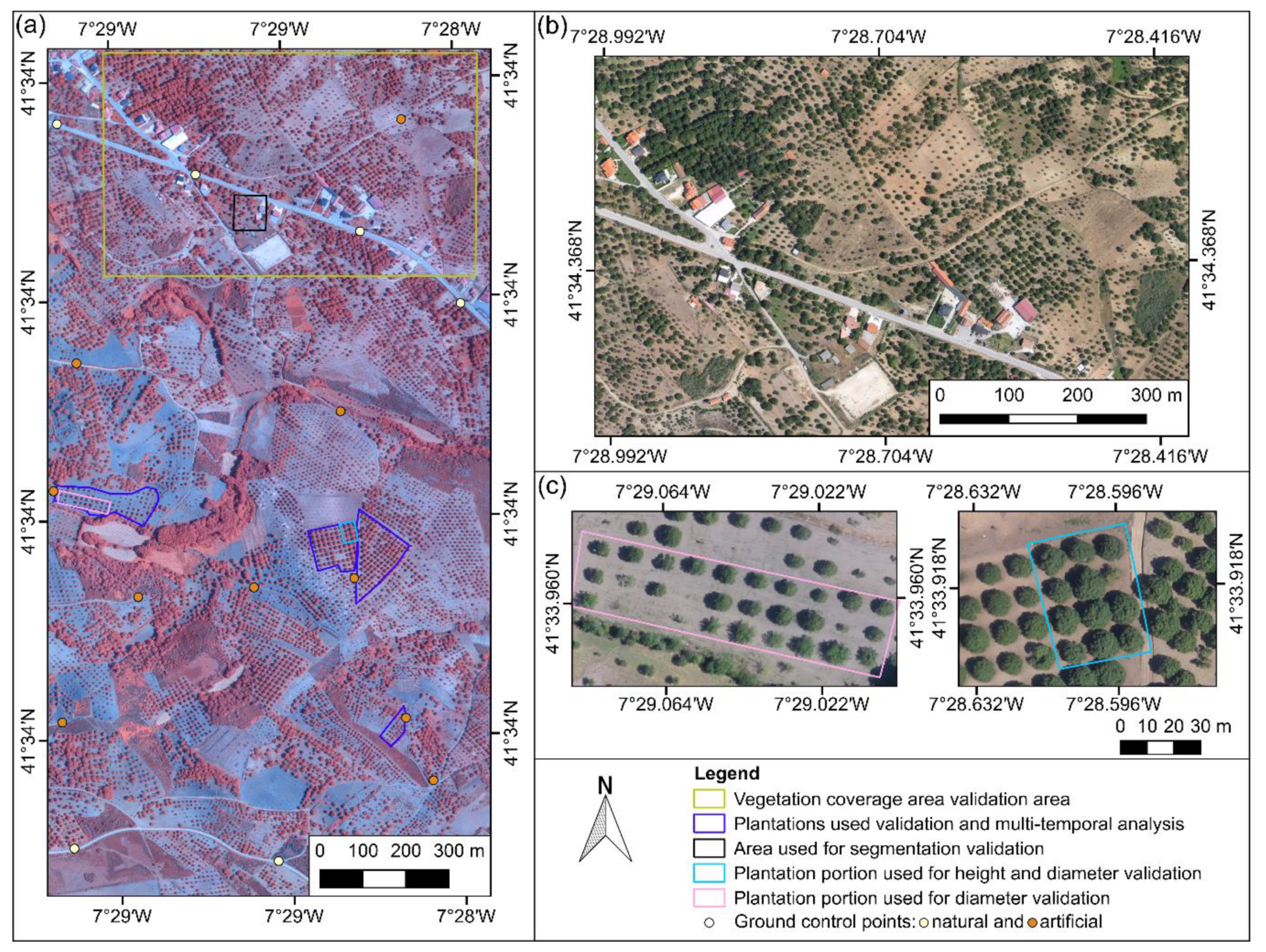
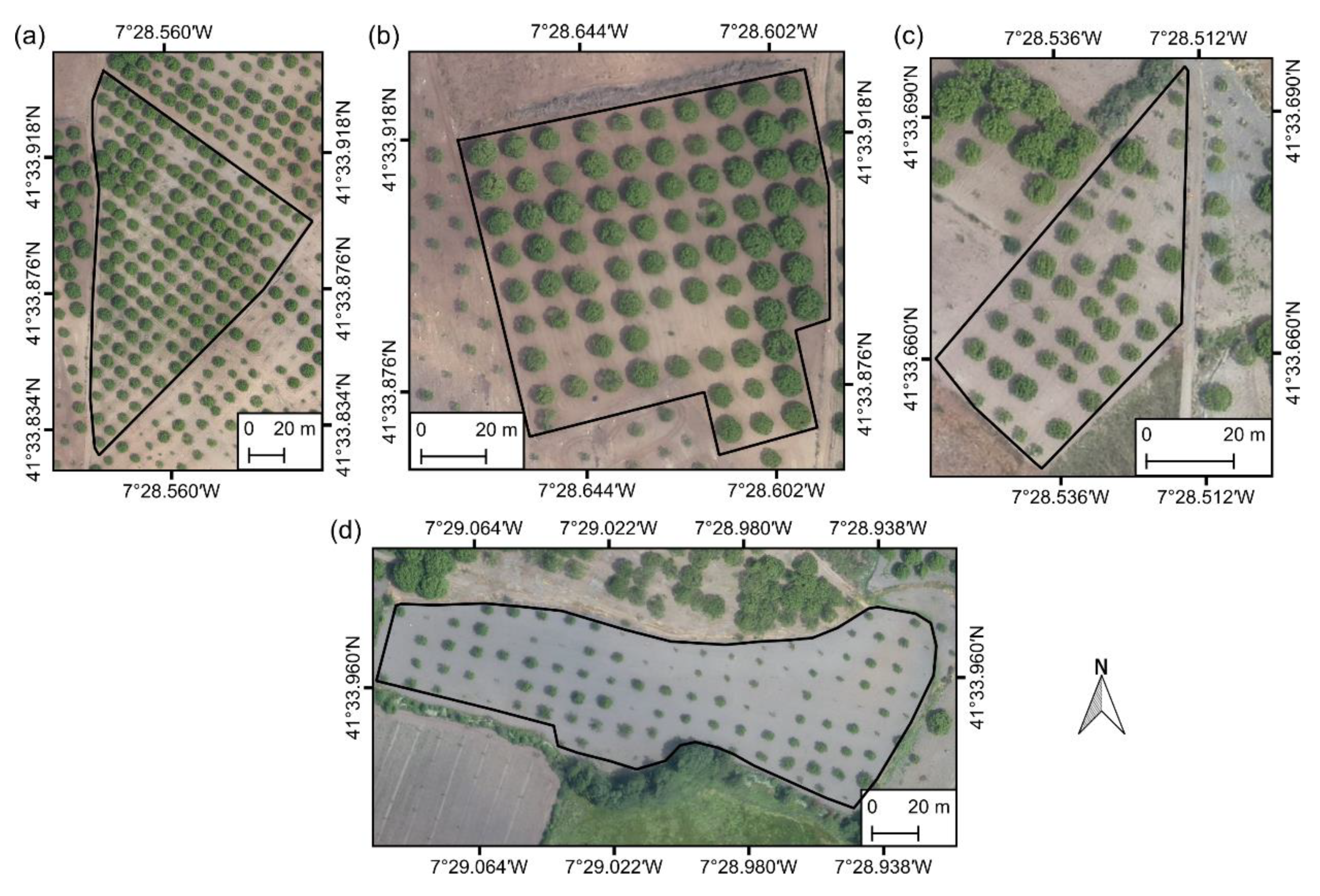
The selection of an UAV for data acquisition is influenced by the specificities of each case study: the size of the area together with UAV’s autonomy influence the ground sample distance (GSD), which may make obtaining an acceptable spatial resolution impossible—this considering, of course, the completion of a single flight. In this specific study, while considering the final purpose of the experiment and the UAV characteristics, a fixed-wing UAV, the senseFly’s eBee (senseFly SA, Lausanne, Switzerland), was used to collect aerial imagery. The flights were conducted over a chestnut trees area (438 ha), located in the Padrela region (Valpaços, Vila Real, Portugal: 41º33′51″N, 7º29′40″W), Trás-os-Montes region (Northeast of Portugal). This region concentrates the highest production of chestnuts in Portugal [20], representing one of the major agronomical sources of income of the region [21]. Specific software was used to plan the flights, wherein the user defines the area of interest, flight direction, longitudinal and lateral overlapping, and GSD (Table 1). At each epoch, two flights respecting the same flight plan were carried out, each one with a different imagery sensor. A standard RGB sensor and a modified sensor were used to collect colour infrared (CIR) imagery in RedEdge (RE), green, and blue bands (Table 1). RE is the spectral region where plant’s reflectance changes from low to high (from 680 nm to 750 nm). These data were acquired on 19 July 2014, 8 September 2015, and 10 July 2017. All of the flights were conducted close to the solar noon time, minimizing shadows, and the same flight plan was used at 550 m height (GSD ~16 cm). Figure 1a presents a general overview of the study area. For validation purposes, an extra flight was conducted in June 2017, using the multi-rotor UAV, DJI Phantom 4 (DJI, Shenzhen, China), in two smaller areas within the study area, as presented in Figure 1c, at 100 m height (GSD ~ 3 cm). Table 1 summarizes the main characteristics of the flight campaigns.
2.2. UAV Imagery Pre-Processing
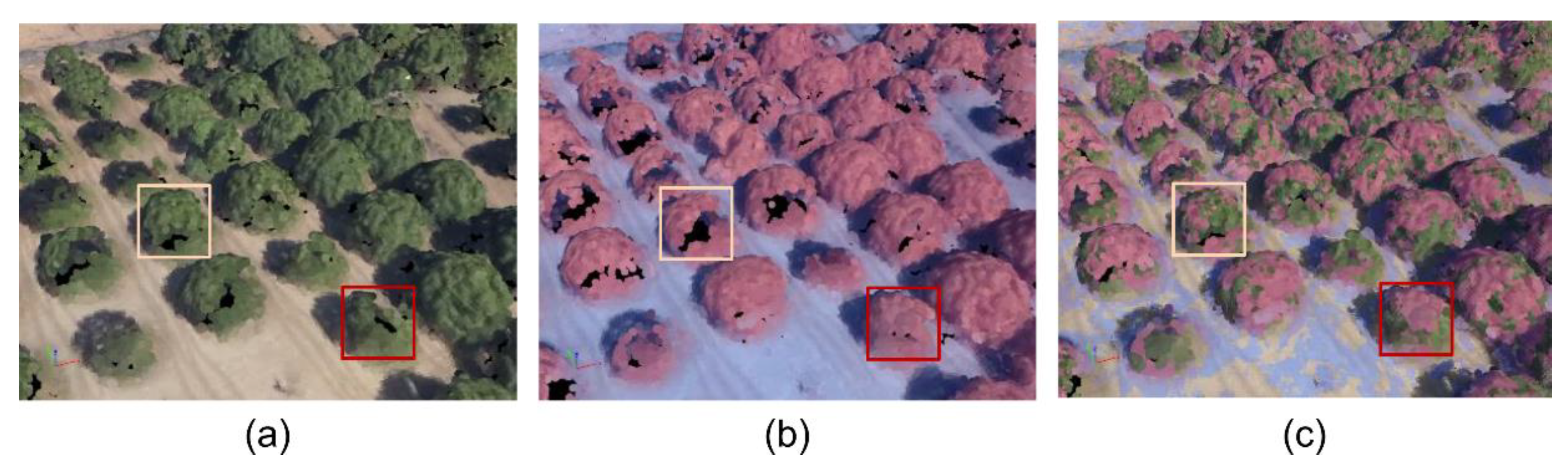
Pix4Dmapper Pro software (Pix4D SA, Lausanne, Switzerland) was used for the photogrammetric processing of the UAV-based imagery. The following processing pipeline was applied: (1) imagery coregistration—data corresponding to each sensor was separately processed in different projects and throughout the identification of common point (tie points), allowing for the generation of a sparse point cloud of the surveyed area, for each sensor’s imagery; (2) project merging—both blocks were aligned relative to each other by using points that are clearly identifiable in the imagery and then merged and geometric correction was applied using ground control points (GCPs), using both natural features and artificial targets that are deployed in the area [19]; (3) dense point clouds computation– two dense point clouds were computed (RGB and RE) using an high point density; (4) point clouds combination—finally, the two sets of point clouds were combined, increasing the total number of points, and ensuring, this way, height information for most of the trees, as shown in Figure 2. Orthorectified mosaics, DSM and DTM were the main outcomes that were generated from this pipeline. Data from each flight campaign has resulted in an excess of area surveyed and different GSDs (Table 1). As such, a section was chosen and resampled to meet the same area (200 ha), as shown in Figure 1a with 16.21 cm GSD.
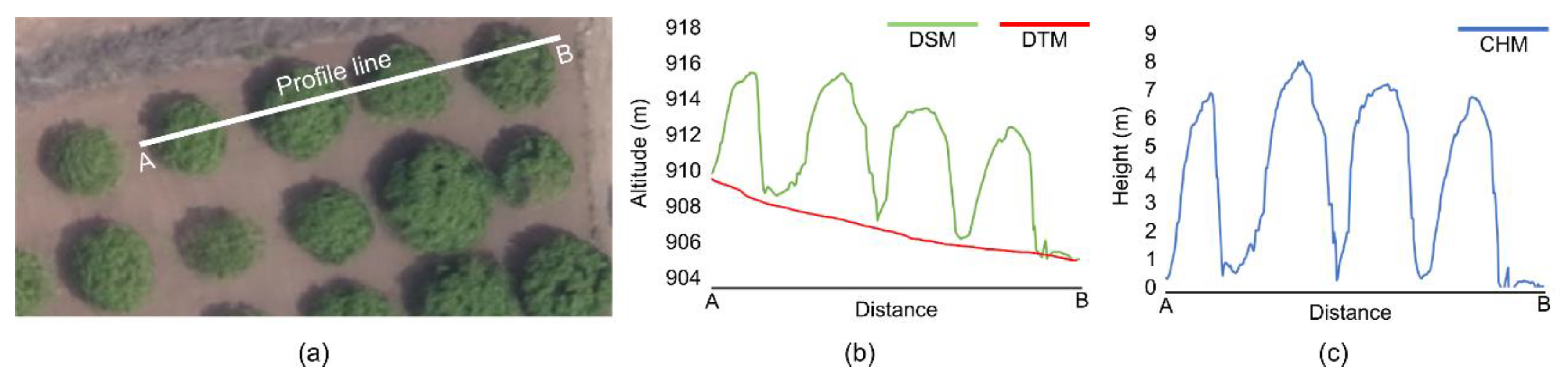
The CHM is computed by subtracting the DTM from the DSM, which makes it almost invariant with respect to terrain’s slope, as illustrated in Figure 3. The use of CHM is crucial, since it allows for obtaining the height of the objects above ground level, enabling the filtering of undergrowth vegetation, such as grass and shrubs, and only analysing the vegetation of interest—in this specific case, chestnut trees.
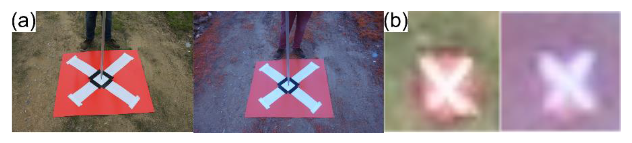
Regarding the geometric correction of the obtained photogrammetric processed data, and from a multi-temporal analysis perspective, it is mandatory to assure a subpixel alignment of all the epochs, otherwise the results may be biased. The used UAVs’ navigation system includes a Global Navigation Satellite System (GNSS) receiver, with a positional accuracy of a few meters. Thus, the georeferencing that is achieved by this equipment does not follow the image’s pixel resolution, only enabling an approximate location. Therefore, it is necessary to use tie points to refine the external camera orientation. Ground Control Points (GCPs) must be distributed throughout the surveyed area in order to avoid significant errors [22]. However, not only should good GCP coverage be done, but also independent check points should be used to verify the quality of the extracted products. In an urban environment, especially when road markings are present, it is relatively easy to find well-defined points that can be used as GCP. However, in the specific case of this study, it was not always possible to apply this method. In fact, only a few areas that were occupied by man-made objects allowed for the identification of such points. As such, the option was to use targets (approximately with 1 m2 area [19]) with centre-marked crosses, placed before the flight at selected locations, and fixed with metal studs (see Figure 4). In total, 16 (6 natural + 10 artificial) GCPs and 20 natural check points were used in every flight.
The imagery geocoding was performed while using the 16 GCPs and the alignment quality assessment was carried out using the 20 check points. For this case study, horizontal check points are the most important, since they allow for controlling the geometric alignment of the different outcomes, which crucial in implementing the multi-temporal analysis. These points are relatively simple to acquire, since surveys of real time kinematic (RTK) GNSS can be quickly acquired in the marked points. A GNSS receiver, in RTK mode, with an accuracy of approximately 2 cm, was used. For a check point of coordinates (E, N), the residuals are calculated by subtracting the coordinates that were measured by GNSS and the corresponding point on the corresponding point interpolated over the reference (ref) orthophoto mosaic. The overall accuracy is given by the root mean square error (RMSE), for the n observed check points, as in Equation (1). The mean and the standard deviation can also be determined to assess whether some systematic trends may exist in the data. However, the final results will not be influenced, since the orthophoto mosaics were independently geocoded and the distribution and geometry of the GCPs remained [23].
Depending on the combinations of campaigns, the reference orthophoto mosaics may vary. The oldest orthophoto mosaics was used as reference and then the differences between the coordinates of the remaining two epochs were computed to assess the geometric quality of the alignment.
2.3. Proposed Method
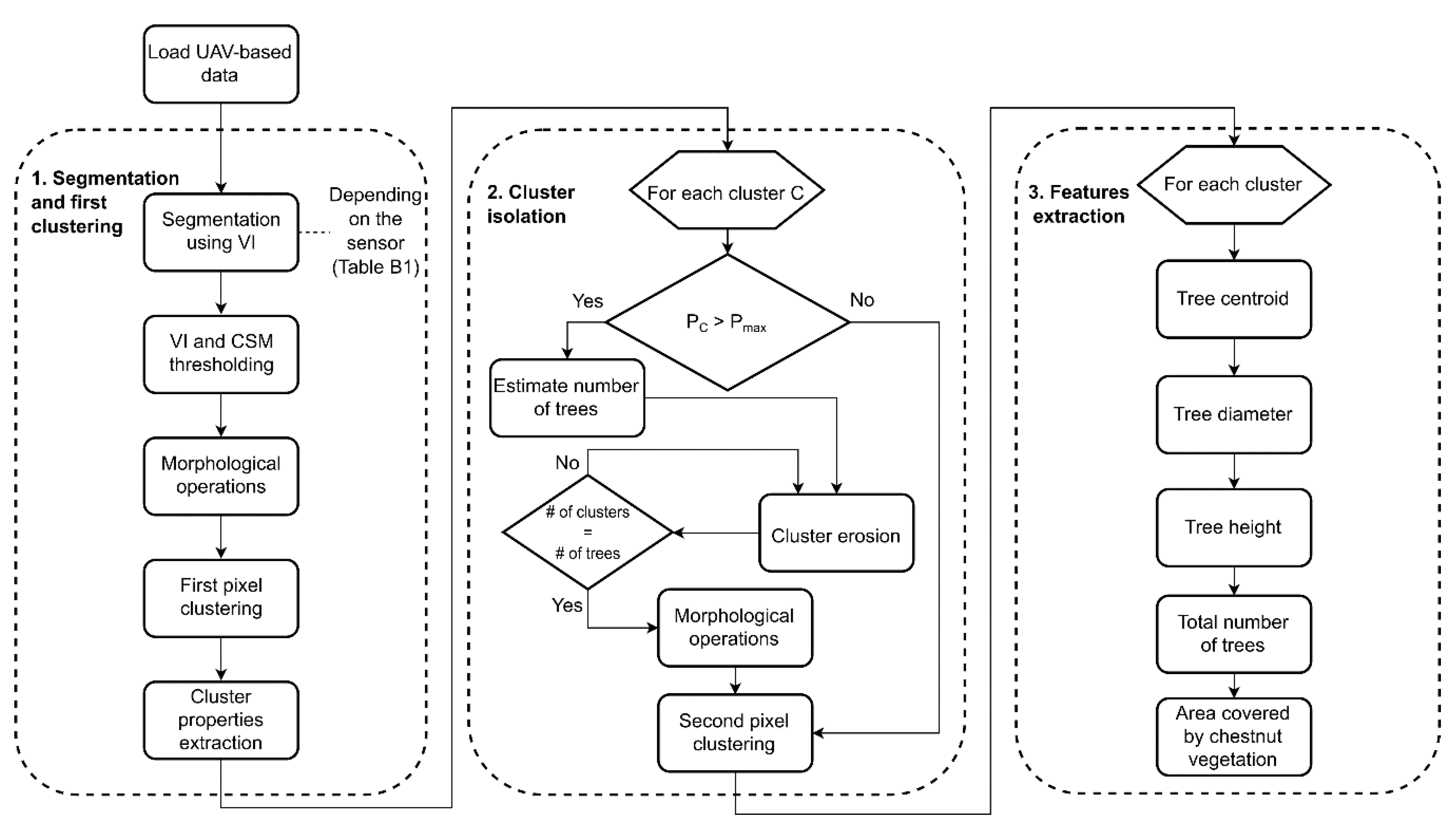
The outputs that are described in Section 2.2 were processed to extract the chestnut trees features. Figure 5 shows the main steps of the method that was developed in this research. The different steps are described in detail in the next sub-sections. Two imagery data sets (RGB and CIR orthophoto mosaics) and the CHM are loaded as inputs to fully exploit the proposed method. It should be noted that the method remains functional, even if RGB or CIR images are individually used as input. This way, the proposed method still fully operational, even in the cases where only imagery resulting from cost-effective platforms, which normally only supports RGB sensors, is available.
In addition, the proposed method also supports multi-temporal analysis, enabling the temporal vegetative evolution monitoring of chestnut plantations.
2.3.1. Segmentation and First Clustering
The first step relies on the preliminary selection of pixels that represent all of the vegetation, mainly associated to chestnut trees. To achieve this, common segmentation thresholding techniques are not appropriate, since those techniques will not distinguish between vegetation and non-vegetation areas, resulting in an image with other objects besides vegetation (e.g., infrastructures, bare soil, roads, and the possible shadowing effects from the chestnut trees canopy). To overcome this issue, the use of broadband spectral VIs was considered. A comparison of different segmentation techniques and vegetation indices was conducted to select the most performant. Appendix A presents the results of this study.
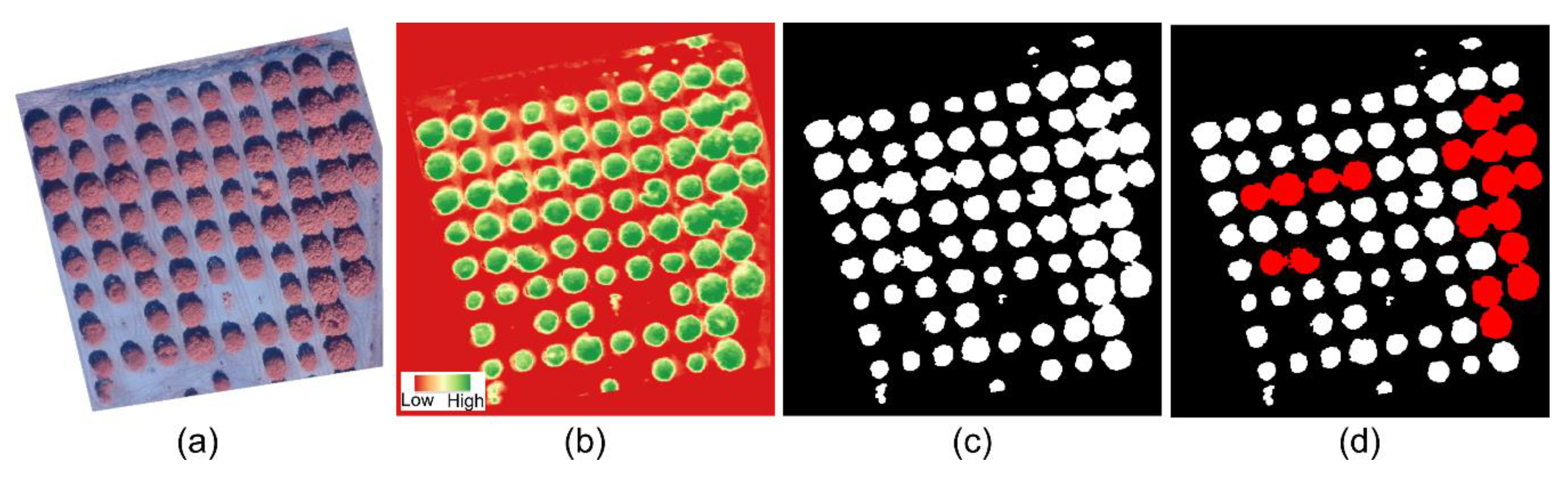
The image resulting from the application of VI-based segmentation (Figure 6b) enables the creation of a vegetation mask by applying the Otsu’s method [24] (Figure 6c). From this selection, a binary image is created that contains all of the pixels that potentially correspond to vegetation. The same approach is applied to the CHM being binarized using a height threshold, then both binary images are joined with a logical AND operation. Next, a set of morphological operations is applied to the thresholding operation result. A 3 × 3 morphological structuring element is used for the open operation (to remove small objects from the foreground), and to the close operation (to remove small holes in the foreground, changing small islands of background into foreground). Thus, the implemented morphological operations allow for simplifying the resultant binary image by improving the detection of sets of interconnected pixels C (i.e., clusters of pixels), forming a set of all clusters , where , which enables the individual analysis of the regions. When located close to each other, the larger trees may be represented as being connected in the binary image (overlapped trees) and, consequently, grouped into the same cluster (Figure 6d).
To prepare the proposed method’s step 2—cluster isolation—a data structure is created with individual cluster parameters. Those parameters are retrieved from the binary image and they are composed of the clusters’ area and centroid. The cluster’s centroid is crucial in associating an identification (ID). At this stage, the cluster’s area value will be used to find clusters that represent inter-connected trees.
2.3.2. Cluster Isolation
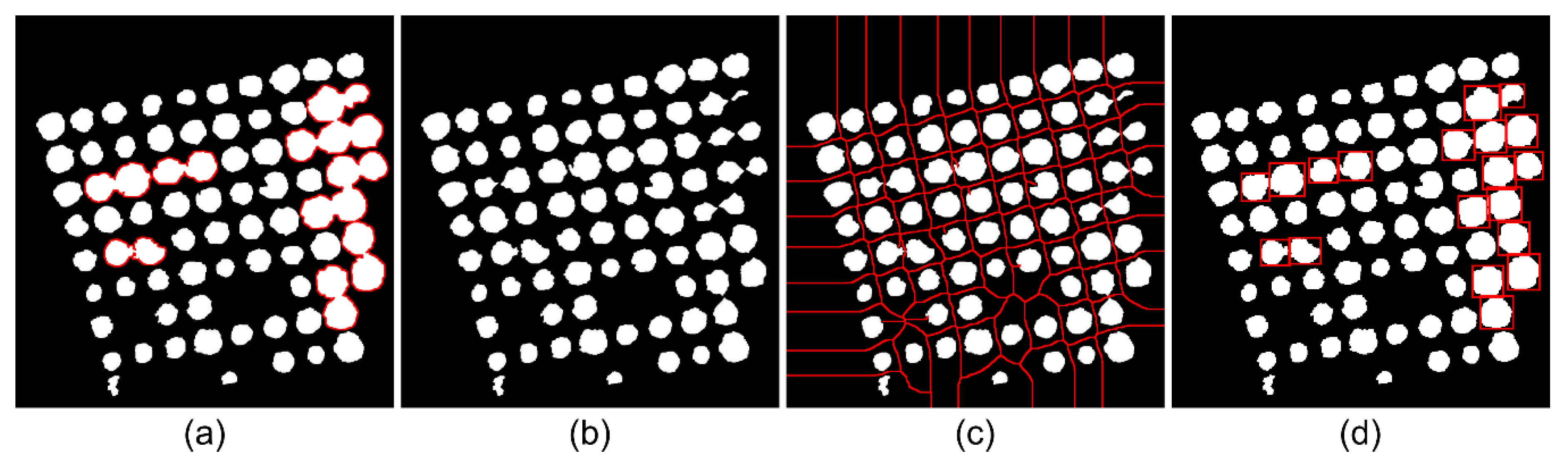
The approach that is applied in the first step of the method can correctly remove most of the non-vegetative areas, allowing for the detection of large vegetation areas. However, even though chestnut trees plantations for chestnut production are usually evenly distributed across the field, their canopy can grow considerably in height and width, forming connected tree crowns, resulting in clusters with interconnected pixels that may include several trees, in the segmented images. Due to this fact, it is necessary to individually distinguish each tree for precise chestnut trees’ monitoring. To achieve this, an individual analysis per cluster C, detected in the first step, needs to be performed. Chestnut plantations generally have a group of trees that typically depict the tree canopy coverage area. As such, the presence of interconnected trees can introduce significant differences on clusters’ area, which can result in a skewed distribution. Therefore, the statistical mode of this set of values—that represents the value appearing most often, i.e., the value that is most likely to be sampled—is determined and a 10% threshold is applied to this value. Clusters’ area mode is used to define the reference area (), which will then be compared—in an iterative process—with the area of each detected cluster . Areas higher than are divided by it, to estimate the number of trees () present in each cluster, as shown in Equation (2). Figure 7a presents an example of clusters meeting this condition.
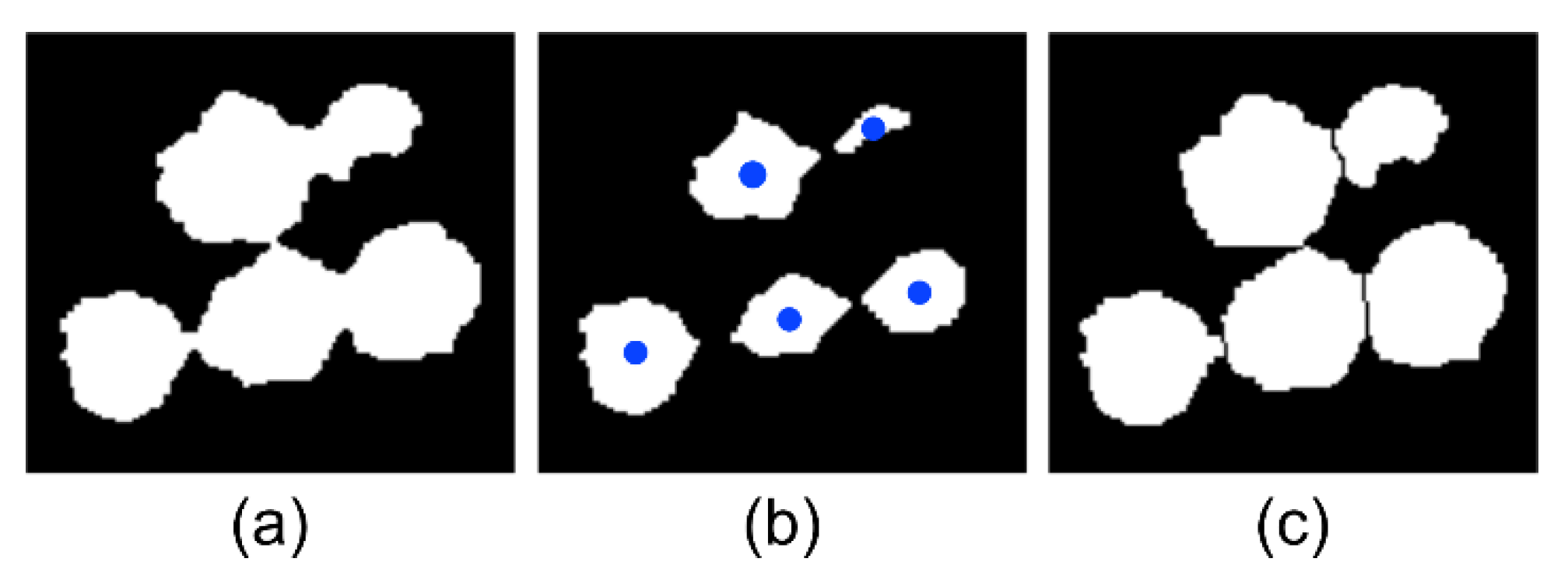
Afterwards, a morphological operation of erosion (see the example of Figure 8) is performed. It consists in interactively removing a line with a pixel thick from the borders, until a new cluster is formed. This new cluster is removed from the selection and the process continues until is achieved (Figure 8b). Finally, the application of the thickening morphological operation to properly separate the clusters by using a one pixel-thick line reverses the process (Figure 8c). This process is achieved by adding pixels to the boundaries of the unconnected clusters (as shown in Figure 7b), nevertheless preserving the total number of clusters, without connecting them. The resulting image is also known as skeleton by zone of influence (SKIZ). Figure 7c presents an example of this operation, being highlighted in red. The SKIZ mask is then used to separate the initially connected clusters by performing per-pixel binary AND operation, resulting in the disconnection of the previously connected clusters. The newly created clusters will be submitted to a second pixel clustering to update the original set, created in step 1. Figure 7d presents the result of this operation, highlighting the separated clusters.
2.3.3. Parameters Extraction
At this point, each cluster corresponds to a single tree and their centroids are used to extract the tree crown diameter, canopy area, and height. Combining the masks that were obtained from the previous pixel clustering process, it is possible to extract the correct parameters from each chestnut tree. Regarding the diameter extraction, the centroids are overlapped to the binary image that was obtained in the method’s second step. The diameter is extracted by measuring each cluster’s Euclidean distances. Thus, the maximum distance is selected and transposed to estimate each tree’s crown diameter. The same approach is applied to obtain the tree’s height. However, the height value is directly extracted from the CHM, by matching the cluster’s centroids with the corresponding CHM and retrieving the maximum value, which is then assumed to be the tree crown’s top. The mean vegetation index value per cluster can also be computed. This value can be interesting to assess chestnut trees vigour and the potential presence of phytosanitary problems.
Furthermore, it is also possible to calculate parameters of the whole plantation, such as the total number of trees and total canopy coverage area and its percentage, by summing out all of the individual areas.
2.3.4. Multi-Temporal Analysis
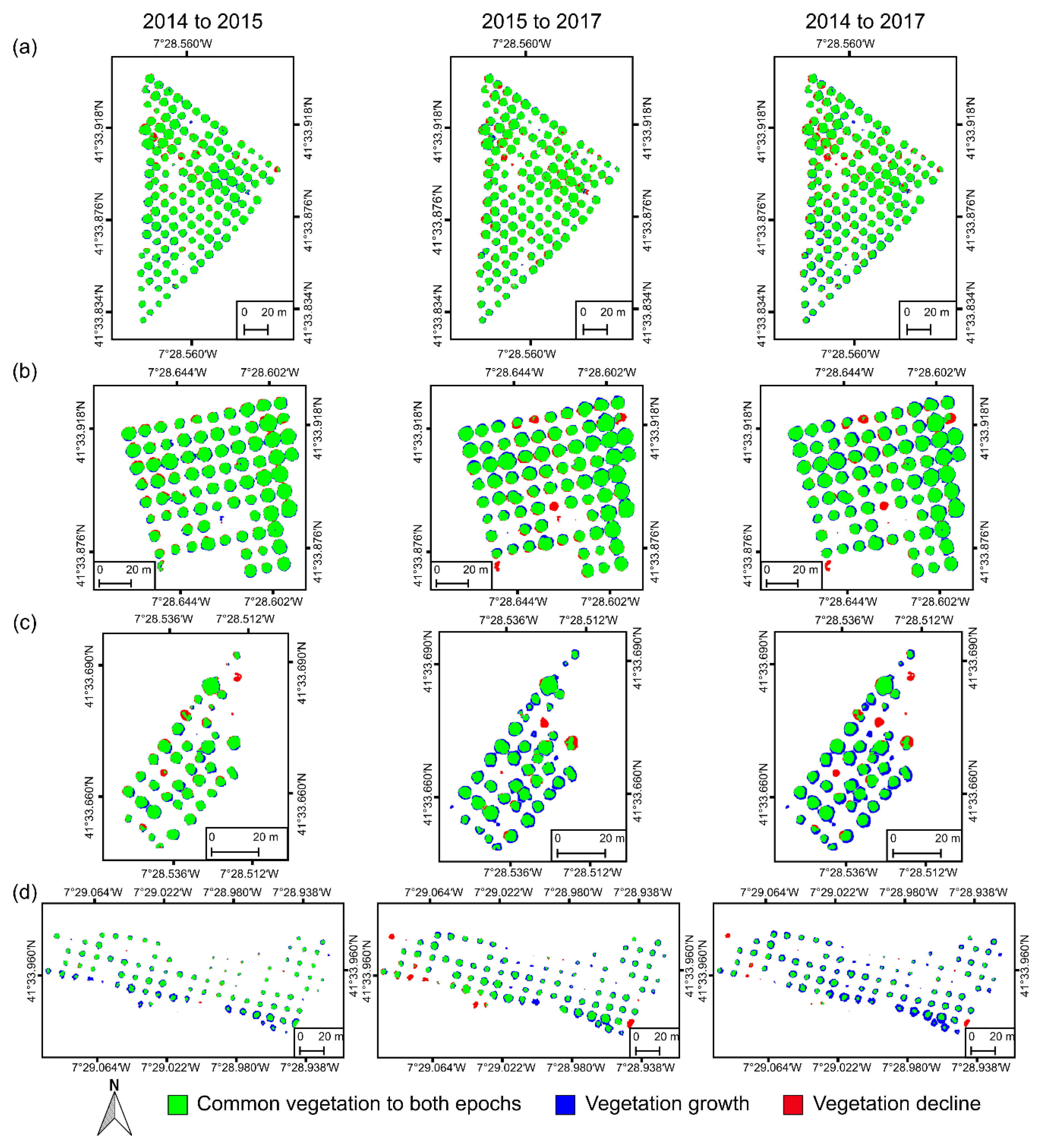
Data acquired in different epochs can be used to create time series, allowing for the comparison between different periods. It is an excellent tool for the management of chestnut plantations, enabling the evaluation of their evolution over time both at the plantation scale and at the individual tree scale. In addition to parameters extraction, it is also possible to detect missing trees and new plantations over the years, through a multi-temporal analysis. This achieved by applying the proposed method to different epochs. By overlapping the detected clusters, missing and new trees can be detected. The implemented multi-temporal analysis can also be performed at the tree crown level. Performing a pixel-wise comparison between the evaluated epochs achieved the chestnut tree canopy growth/decline. The following scenarios may occur: (1) common vegetation in both epochs—vegetation is present in both epochs in the same pixel (i,j) coordinates; (2) vegetation growth—vegetation is not detected in the first epoch, but it is detected in the second epoch, meaning a chestnut tree growth; and, (3) vegetation decline—pixels considered as vegetation in the first epoch that were not represented in the second epoch. Chestnut trees with a decline percentage greater than 15% are signalled as potentially having phytosanitary problems, meaning that they need to be inspected in the field, reducing time-consuming and laborious field inspections. Therefore, these results can be analysed both at a plantation level and at the individual tree level.
2.4. Validation
To validate the proposed method and the feasibility of the data that was obtained from photogrammetric processing of the UAV-based imagery, different tests were conducted for different parameters, namely: VI selection; vegetation coverage area assessment; number of detected trees; and, tree crown diameter and tree height estimation. This way, five test areas were selected for this purpose. All of the chestnut trees present within each area were manually segmented for validation purposes. The first test area represents about 23% of the whole surveyed area (46.89 ha), as presented in Figure 1b. The area was selected, since it includes several types of elements/objects. Beyond recently planted chestnut trees, non-controlled chestnut plantations, several vegetation outliers (e.g., lawns), and infrastructures, such as buildings and roads cover the area. It was considered to analyse the general behaviour of the method when facing outliers and it was only tested in vegetation coverage area. Apart from this area and since the proposed method focus is the monitoring of chestnut plantations, four other chestnut plantations were selected and analysed as the test areas (Figure 9). Plantation #1 (Figure 9a) has approximately 1.45 ha, Plantation #2 (Figure 9b) has 1 ha, Plantation #3 (Figure 9c) has an area of 0.26 ha, and the area of Plantation #4 (Figure 9d) is about 1.3 ha. While Plantations #1 and #2 are composed of fully developed chestnut trees, Plantation #3 has chestnut trees at different development stages and Plantation #4 is mainly composed of more recent chestnut trees. These four areas were used for determining the area coverage, assessing the number of trees detected, and for selecting the optimal vegetation indices (Appendix B). Reference masks of these areas were manually created for the three available flight campaigns.
2.4.1. Vegetation Coverage Area
The purpose of this validation is to evaluate the behaviour of the proposed method in the detection of chestnut trees vegetation. The method was applied in a large and heterogeneous area (Figure 1b) with different vegetation covers, in an uncontrolled environment, and to four different plantations (Figure 9). The computational time of the algorithm to perform in the complex area was measured to be compared with the time that is required to manually create the reference mask of the same area. Validation was conducted comparing the method’s obtained results with the binary images that were created from the manual segmentation. This way, each pixel (i,j) was analysed, and it is classified as being true and false positive (TP/FP, exact/over detection), which refer to the number of correct/incorrect pixels that are classified as chestnut vegetation and similarly true and false negatives (TN/FN, exact/under detection) for non-chestnut trees vegetation. For this purpose, different parameters were evaluated, namely: producer’s accuracy, user’s accuracy, and the overall accuracy. Producer’s accuracy is obtained by the percentage of how many pixels on the map are correctly labelled as corresponding to chestnut and to non-chestnut vegetation, encompassing errors of omission. User’s accuracy is obtained by the percentage of all pixels that were identified as a chestnut and non-chestnut vegetation that were correctly identified, encompassing errors of commission.
2.4.2. Number of Detected Trees
This validation consisted in the comparison of the number of trees that were detected by the proposed method with the real number existing into a specific plantation at a specific epoch. Since the area that is used for vegetation detection validation contains thousands of trees, which makes the segmentation difficult, it was decided to use a controlled environment consisting of the four different plantations (Figure 9). The selection was done assuring the representativeness of most real cases present in the study area.
In what regards this validation, different parameters were evaluated: (1) good detection—the three was correctly detected when compared with the reference mask; (2) missed detection—the tree was not detected; (3) extra detection—corresponding to a wrongly detected chestnut tree; (4) over detection—a single chestnut tree being classified in multiple clusters; (5) under-detection—multiple trees classified in a single cluster; (6) larger detection—tree is larger than its actual size; and, (7) smaller detection—chestnut tree is smaller than its actual size.
2.4.3. Tree Height and Crow Diameter Estimation
To validate trees height estimation, 12 chestnut trees, as presented in the right side of Figure 1c, were measured in the terrain using a laser rangefinder with a precision of ± 20 cm (TruPulse 200, Laser Technology, Inc., Colorado, United States of America). Chestnut experts from University of Trás-os-Montes e Alto Douro have consistently monitored Padrela’s region regarding chestnut trees cultural practices, environmental context, phytosanitary conditions, and an evolution, in recent decades. This monitoring activity resulted in several publications [1,7,19,25,26,27,28,29,30], which conclude that both cultural practices and environmental context are identical throughout the region. Therefore, the 12 trees selected from plantation #2—the selection was made based on the main characteristics of an adult chestnut tree, well represented in this Plantation—can be considered representative for the entire area under study. Regarding tree crown diameter estimation validation, two groups of trees were selected: the 12 trees that were used for the tree height estimation validation composed the first group and 28 chestnut trees composed the second group (both areas presented in Figure 1c). These measurements were obtained in the 2017 flight campaign day. Tree crown diameter were obtained by tape measuring. Two measurements were considered that corresponded to the four quadrants and the mean value was used as ground-truth. These values were compared with those that were estimated from the proposed method. Finally, a comparison was performed and the overall agreement between the observed in-field measurements (o) and the root mean square error (RMSE) verified the estimated values (e), as in Equation (3), where n represents the total number of analysed trees. In general, RMSE is a good metric to evaluate (punctually) the quality of the method’s measurements.
The coefficient of determination (R2), which consists in a statistical measure of how close the data is to the fitted regression line, was also calculated.
3. Results
This section presents the results of accomplishing the validation procedures that are described in Section 2.4, concerning the proposed method’s validation and extracted features reliability. Moreover, a multi-temporal analysis, by applying the proposed method to four chestnut plantations in three different epochs, is also presented.
3.1. Data Alignment
Table 2 presents data from the three campaigns combinations, namely the results from their accuracy analysis. Analysing the values that were obtained for the residuals mean and standard deviation—the mean value is close to zero meters and standard deviation is lower than RMSE—means that there are no systematic errors. The results presented in Table 2 also allows to conclude that the geometric adjustment between epochs is very similar in less than one pixel. These results validate the multi-temporal analysis that is performed by applying the proposed method.
3.2. Vegetation Coverage Area
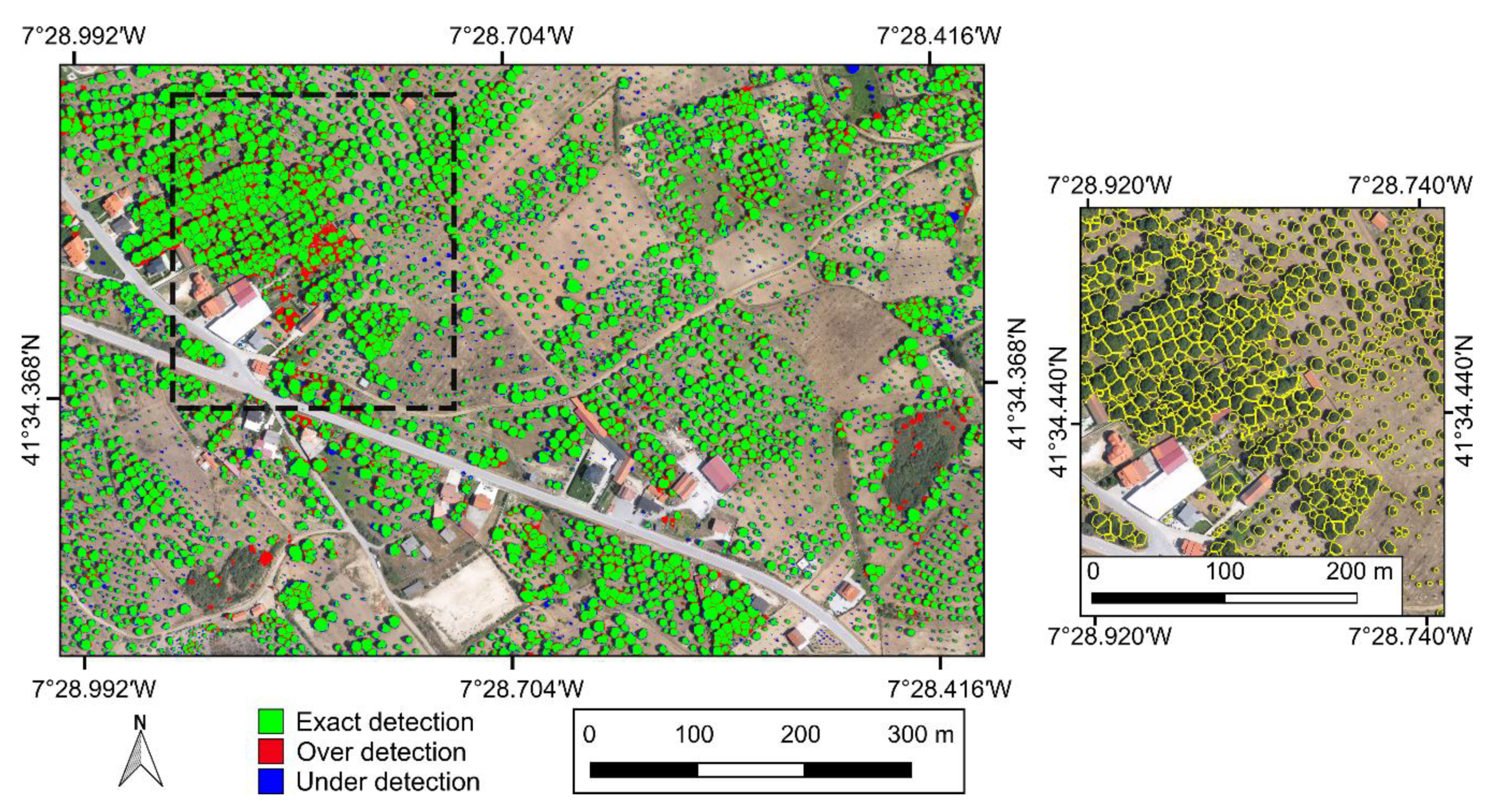
Figure 10 illustrates the result of the proposed method, when compared with the manual segmented image, in an uncontrolled environment (RGB representation presented in Figure 1b). The proposed method obtained 94.31% of exact detection and an error rate of 5.69%, from which 3.05% is of under detection (FN) and 2.63% over detection (FP).
According to the manual binary mask, in a total area of 48.2 ha, only 12 ha contains chestnut trees, corresponding to 25% of the total area. From this area, the proposed method identified 12.2 ha of chestnuts trees, which corresponded to an over estimation of 1.6%. Producer’s accuracy was around 88% and user’s accuracy is 89.5% (see Table 3 for further results).
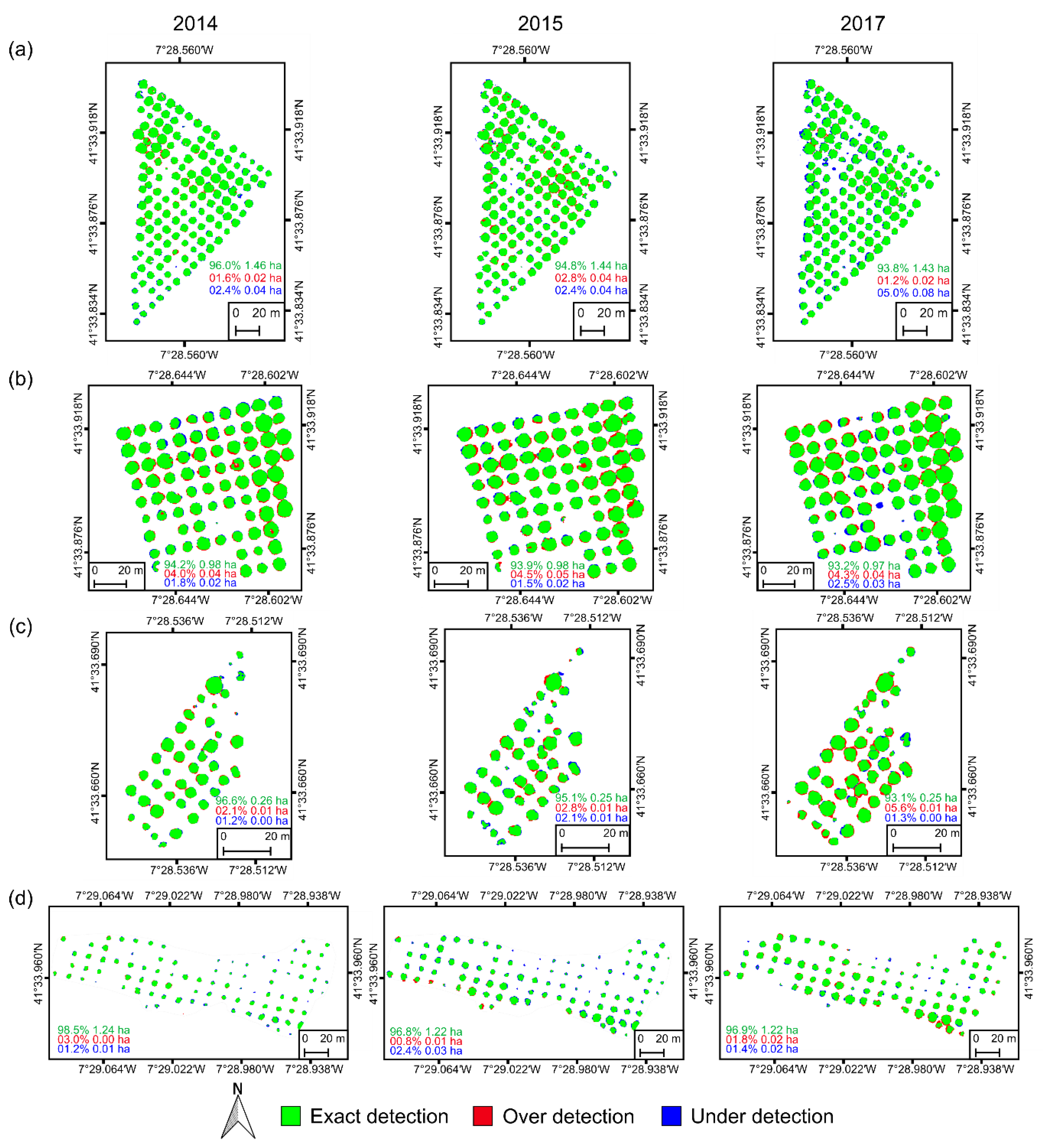
For reference, the manual mask was created in eight hours, while the method was performed in approximately 10 min using a laptop computer with an Intel core I7-4720HQ CPU @ 2.6 GHz, 8 GB of RAM, a NVIDIA GeForce GTX 950 GPU with 2 GB of dedicated memory, and a 700 GB HDD. For a more realistic study, four chestnut plantations, as presented in Figure 9, were selected for evaluation. Figure 11 shows a visual interpretation of the results. Table 3 provides the results per plantation, in each epoch, for the parameters that were considered in this evaluation. Producer’s and user’s accuracy was only evaluated for chestnut vegetation class. Regarding, the non-chestnut vegetation class was not deeply analysed, but it was higher than 95% in most of cases, with a mean of 97% for producer’s accuracy and 96% for User’s accuracy.
When analysing the four chestnut plantations in the three epochs, the mean overall detection reaches 95%. Evaluating these results in a plantation basis, higher detection values were observed in plantation #4 (97.4%) and lower in plantation #2, with 93.8%. The remaining plantations reached accuracies of around 95%. When observing results by epoch, the highest detection rates were obtained in 2014 (96.3%), whereas 2017 reached the lower mean values (94.2%). As for the 2015 flight campaign, its mean accuracy value was of 95.2%. The higher values were obtained for plantation #4, in 2014, and the lowest was 93.1%, for plantation #3. As such, it can be stated that the method is suitable for chestnut detection, with accuracy greater than 93% and varying up to approximately 99%, depending on the plantation characteristics.
3.3. Number of Detected Trees
To evaluate the number of trees detected by the proposed method, the same test plantations that are presented in Figure 9 (see Figure 1 for location) were used. The results were compared with the manual counting of the number of trees present in the plantations and the three epochs (2014, 2015, and 2017) were evaluated. Table 4 presents the obtained results, per plantation in each epoch.
In total, 1092 chestnut trees were included in the analysis. The proposed method was able to detect 1074 chestnut trees. However, six of those corresponded to wrongly estimated trees (approximately 0.5%), i.e., trees classified as extra, over or under detections. Globally, 1068 trees were correctly classified, representing an accuracy rate of about 98%. This way, exclusively concerning the detection of chestnut trees (i.e., good, larger, and smaller detections), the method has a mean classification of 99%, per flight campaign. Regarding this detection in a plantation basis, the mean accuracy of all flight campaigns is also of about 99%, being the lower value corresponding to plantation #3 (approximately 97%). Moreover, no cases of wrongly estimated trees (extra detections) were observed. In total, 19 chestnut trees were not detected (1.7%).
3.4. Tree Height and Crow Diameter Estimation
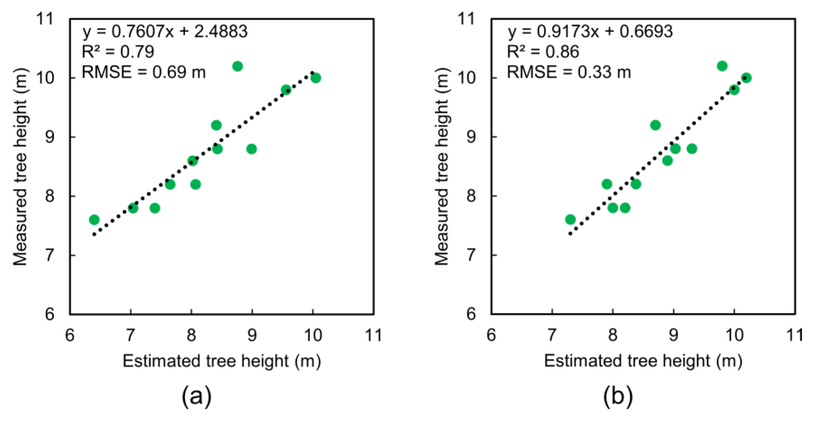
Figure 12 presents the results that show the relationship agreement between in-field measurements (ground-truth data) and the measurements that were estimated by applying the proposed method. The height values ranged from 7.6 m to 10.2 m, with a mean value of 8.8 m. For the model with 16 cm GSD (Figure 12a), the linear regression presents a R2 = 0.79 and a RMSE of 0.69 m, and the estimated maximum, minimum, and mean values were 10 m, 6.4 m, and 8.2 m, respectively. Using data resulting from a flight at lower height, there was a significant increase in this parameter accuracy. Indeed, to test the influence of the flight height in tree’s height estimation, a 100 m height (GSD ~ 3 cm) flight was carried out with DJI Phantom 4, in the same area. In this case, the accuracy significantly improved—R2 = 0.86 with a RMSE of 0.33 m (Figure 12b), the maximum, minimum, and mean height values were also closer to the measured values, being, respectively, 10.2 m, 7.3 m, and 8.8 m.
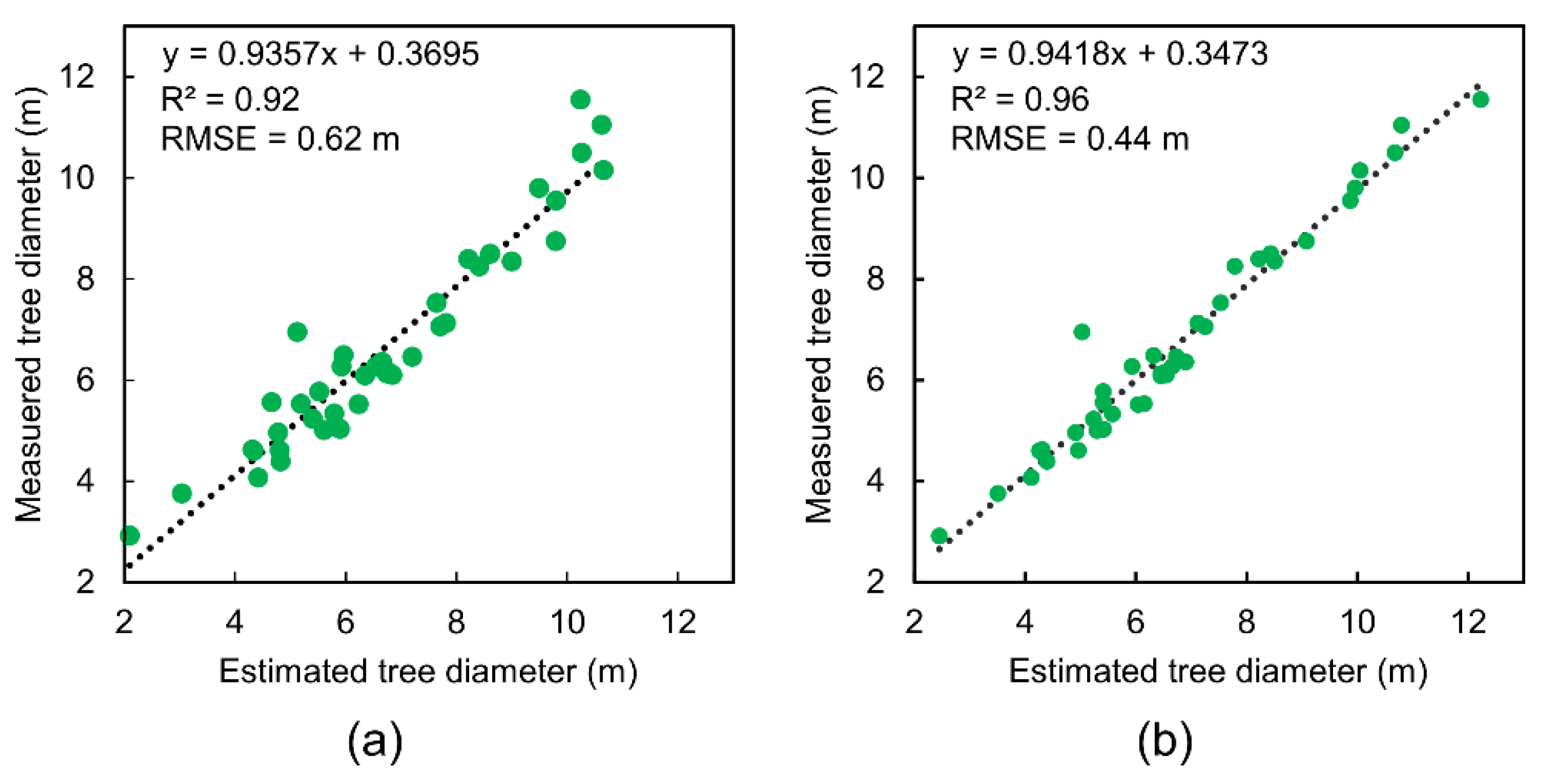
Concerning tree diameter validation, analogously to tree height validation, the estimated diameter values that were obtained from the proposed method were compared with ground-truth data, where the 40 chestnut trees’ diameter ranged from 2.45 m to 12.23 m, with a mean value of 6.71 m. Figure 13 presents the relationship between in-field measurements and those that were estimated by the proposed method. From the data acquired at 550 m (GSD ~ 16 cm), the linear regression presents a R2 = 0.92 (Figure 13a), which indicates that the estimated tree crown diameter fits the real data in an 92% accuracy rate. As for the RMSE value, an error of 0.44 m was obtained. Regarding the minimum, maximum, and mean values that were estimated from the 16 cm GSD data were 2.1 m, 10.66 m, and 6.73 m, respectively. Concerning tree’s crown diameter estimation that was obtained when using the flight conducted at 100 m height (GSD ~ 3 cm), similarly to tree height estimation, there was an improvement in this parameter (see Figure 13b). The linear regression presents a R2 = 0.96 and the RMSE shows a value of 0.44 m, minimum, maximum, and the mean estimated values were, respectively, 2.92 m, 11.55 m, and 6.67 m.
3.5. Multi-Temporal Analysis
One of the major advantages of the proposed method, compared to the actual state of the art, consists of its capacity to perform multi-temporal analysis, both at the tree and plantation levels.
3.5.1. Plantation-Level Analysis
The data available from the 2014, 2015, and 2017 campaigns was used to perform a multi-temporal analysis. The number of chestnut trees in the plantation and their respective coverage areas were compared. The same plantations that are presented in Figure 9 (see Figure 1 for location) were used. Table 5 shows the occupation area of the chestnut trees in the four plantations for each flight campaign, along with the mean values of tree height, canopy diameter, and area. Figure 14 shows the evolution over time of the four chestnut plantations, representing the differences between 2014–2015, 2015–2017, and 2014–2017 campaigns.
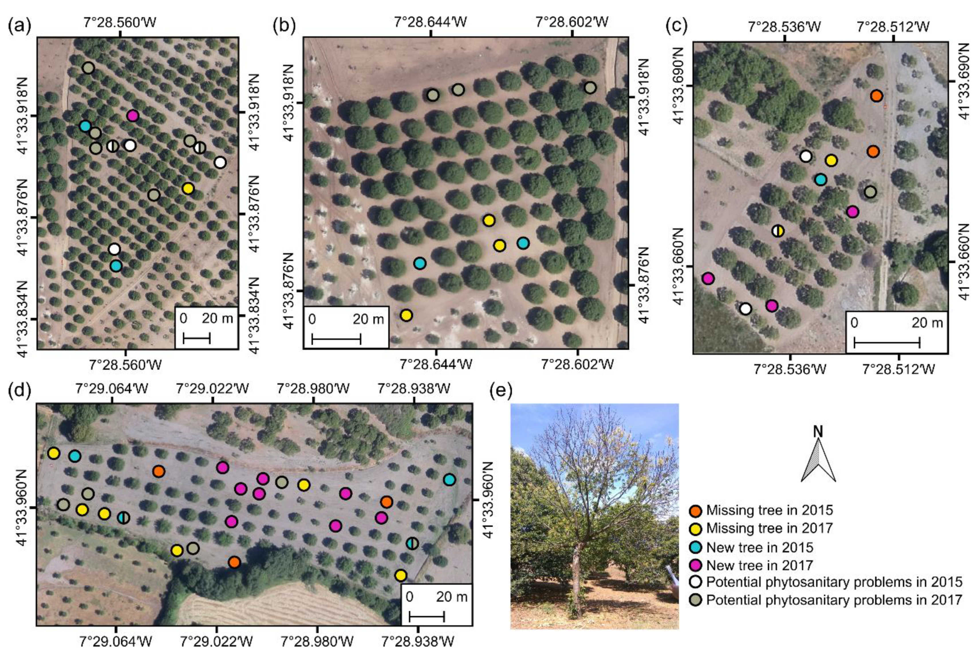
Regarding the number of trees (Figure 15), plantation #4 presented more changes during the analysed period, constituting a total of 20 new or missing chestnut trees (10 new trees and 10 missing trees). Plantation #1 presented a total of four changes: a missing tree and a new tree were detected in the 2017 period; two new trees were also detected in the 2015 period. Five changes were observed in plantation #2: two new trees were detected in 2015; and, three were considered as missing in 2017. When considering plantation #3, four chestnut trees were considered missing, two in each period (2015 and 2017), and four new trees were detected, one in 2015 and three in 2017, performing a total of eight changes. Potential phytosanitary problems were also detected in all of the analysed plantations.
3.5.2. Tree-Level Analysis
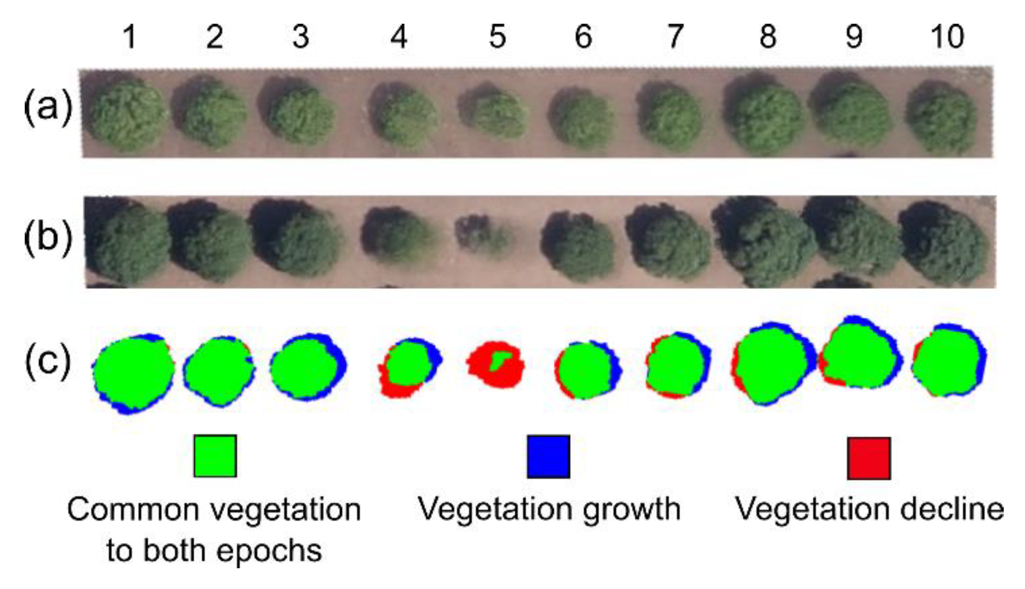
The proposed method is also able to perform a multi-temporal analysis at the tree-level. This is only possible due to method’s step 3—cluster isolation—where the trees are properly separated. To illustrate the method’s performance, Figure 16 highlighted the results of ten trees. Those trees refer to the line of trees that is present in the top of plantation #2 (Figure 9b) and it is used to illustrate the behaviour of the proposed method.
Table 6 presents the quantitative results obtained from applying the proposed method to the ten trees selected.
4. Discussion
4.1. Vegetation Coverage Area
The method achieved good overall results, even in the presence of a complex and larger scenario (Figure 11), which constitutes an extreme limit situation. For the complex area (Figure 1b), there was a slight tendency for the method to overestimate chestnut vegetation rather than underestimate it. Still, both of the values are around 11%. Concerning these errors, it was observed that a large part of the over detection is related to the difficulty of discriminating some lawns—since there were trees within the lawns—and due to some undergrowth, which have a considerable height in the CHM, making it difficult to discriminate. This was also reported in [31]. Regarding under detection, some errors were observed on the VI in trees that had few leaves and from the CHM in some recent chestnut trees where the height information was not representative, causing misclassifications from the method. These problems persist, even when considering higher resolution UAV-based imagery [32,33]. Probably, those trees may be misclassified due to the absence of leaves, while considering the imagery resolution. At the same time, this fact may be used in a multi-temporal approach to highlight the trees that are potentially affected by phytosanitary problems. An important aspect is that non-vegetation features present in this area were correctly classified as being so, which includes most of undergrowth vegetation and infrastructures as buildings, which have height values that are similar to some chestnut trees.
It is worth noting that this large area (Figure 1b) is not representative of a chestnut plantation used for economic purposes. Indeed, most chestnut plantations, namely the more recent ones, follow a well-defined alignment. In these cases, the method’s performance reaches higher overall accuracies (93 to 99%). However, when excluding non-chestnut vegetation (true negatives: soil and undergrowth vegetation), the results differ from the overall accuracy. When considering the producer’s accuracy, its mean value is 90.7%, being that the higher and lower values were reached in the 2017 campaign, for plantations #1 (96.6%) and #4 (88.1%), respectively. When analysing the results in a plantation-basis, plantation #1 obtained the higher values in this parameter (94.7%), while plantation #3 obtained the lowest producer’s accuracy (87.3%). When considering the producer’s accuracy per epoch, this value is closer, with lower precision in 2017 (89.3%), while the higher values were obtained in 2014 (92.5%). In 2015, this value was of 90.4%. As for user’s accuracy, which encompasses all chestnut vegetation present in the image (i.e., also considers chestnut vegetation classified as being not), plantation #4 is the most influenced by these errors (mean of 85.0%). This fact can be related with the type of trees present in this plantation—more recent than other plantations—and due to the lack of pixels that represent each tree at this GSD, which caused the method to not detect part of the canopies. On the other hand, plantation #2 provided higher rates in all of the seasons, with a mean value of 94.8%. The epoch with lower user’s accuracy was 2015 (90.1%), followed by 2014 (91.65%) and 2017 (91.7%).
Despite the mean user’s and producer’s accuracy values being similar (~91%), it can be sated that the method tends to overestimate chestnut vegetation (FP), rather than underestimate it (FN). Plantation #1 was the less influenced by FP and FN, while plantation #4 was the most influenced, especially by FN. These results clearly contrast with the ones that were obtained in the overall accuracy, where plantation #4 obtained higher overall accuracy (97.4%) the remaining with accuracy around 94% to 95%. If only accuracy was analysed, the results could be wrongly interpreted, since the non-chestnut part in some plantations is considerably higher than other plantations. Indeed, the area of FN and FP is not so different and is, in most of the cases, mainly located in the borders of canopies. This way, when considering the obtained results, it can be pointed out that plantation #1 was the area with the best results, while plantation #4 was the less performant in chestnut vegetation detection. Nevertheless, another aspect is that reference masks were manually created, which means that small errors can be present.
The proposed methodology was developed with the underlying premise that it was to be used to detect and monitor chestnut trees plantations whose own characteristics and those of the trees that constitute them lead to few crown overlaps. Nevertheless, regular development of trees may bring—even when regarding with ordered plantations—canopy overlaps. These are well resolved by applying the proposed method (Figure 8). The study area also has some older (and therefore disordered) chestnut plantations, where the proposed method presented high precision results (Figure 10 right). As such, the proposed method may be potentially adapted to other plantation types. Nevertheless, further studies are needed to evaluate this issue.
4.2. Number of Detected Trees
Despite the high accuracy in the results that was obtained in the evaluation of this parameter (presented in Table 3), some trees were not detected, mostly in cases where trees crown was too small. This is the case of plantation #4, where the missing detection reached a mean value of 5%, when considering the three epochs. Being this mainly related to the used data, since flights were performed at 550 m height, making these small trees almost imperceptible in the image. Moreover, detection also fails when the trees present few or no foliage due to phytosanitary problems, making it almost impracticable to detect canopy vegetation through VIs. This is the case of a tree with considerable size (approximately 50 m2), which was not detected in plantation #2 on the flight campaign of 2017 (see Figure 11b right). However, this apparent limitation constitutes a strong point of the method, since when applied in a temporal perspective, it allows for the detection of trees that are potentially affected by phytosanitary phenomena. As for over detection cases, these are related to the method’s cluster separation in chestnut trees that had an irregular canopy shape, causing it to be divided into multiple clusters. However, the number of cases is relatively small (mean of 0.3%). In regards to under detection, it was only verified in plantation #3, being caused by a small tree adjacent to a considerably larger tree. Larger detections mainly occurred in chestnut trees with a considerable canopy area (see Figure 11b), in the other hand, smaller detections cases were observed in smaller chestnut trees (see Figure 11d). The proposed method accuracy is above or in line with the existing similar methods for tree detection. In Mohan et al. [12], an open canopy mixed conifer forest was surveyed and a total of 312 trees were detected by their method, from a total of 367 reference trees with an accuracy of 85%, missing 55 trees. However, 46 trees were over detected, performing a total of 358 trees. Ok and Ozdarici-Ok [18] evaluated individual citrus trees delineation from UAV-based DSMs, and an overall precision of 91.1% in a pixel-based analysis and 97.5% in the object-based analysis was obtained by the method. The results from the proposed method are also greater or in line with the ones that were obtained from the application of complex and expansive LIDAR data [15,16].
4.3. Tree Height and Crow Diameter Estimation
The results that were obtained for tree height and crown diameter estimation are in line or even better than the ones from another studies. Tree height estimation was the less accurate when comparing both parameters. However, when considering that the instrument used in the measurements has an intrinsic error of about 20 cm, this accuracy is perfectly acceptable [12]. Moreover, some errors can be related to the used digital elevation models, since the flight was performed at 550 m height (GSD ~16 cm). When considering the differences for the flight performed at 100 m height (GSD ~3 cm), as expected, there is a direct correlation between height accuracy and image resolution: the better the spatial resolution the better the reached accuracy. It is worth noticing that, in most cases, the flight height will be lower than 120 m (UAV regulations [34]), which assures the method’s effectiveness, even in the estimation of trees’ height. The results prove the effectiveness of the proposed method in the estimation of structural properties (tree height and canopy diameter) of chestnut trees, with a good hit rate and with a relatively low error. Zarco-Tejada et al. [11] conducted a tree height assessment of 152 olive trees, with heights that range between 1.16 and 4.38 m, a R2 = 0.83 and a RMSE of 35 cm was obtained. Similarly, to this study, the results tended to be less precise in lower spatial resolutions. Panagiotidis et al. [35] obtained a R2 = 0.72 to 0.75 and RMSEs of 3 m in two plots (48 and 39 trees, ranging from 15 to 35 m). As for tree crown diameter a RMSE of 0.82 and 1.04 m and R2 = 0.63 and 0.85, for plot 1 and 2, respectively, with a diameter varying from 11 to 19 m. Díaz-Varela et al. [36] acquired UAV-based imagery to estimate parameters from olives (150 trees, heights ranging between 1 and 3 m) with 7 cm GSD, obtaining a RMSE of 0.45 (R2 = 0.07) for tree height and for tree crown diameter obtained an RMSE of 0.32 (R2 = 0.58), with values that range from 1 to 2.5 m. Lim et al. [37] evaluated tree detection using DSM from photogrammetric processing of UAV-based imagery, and obtained a RMSE of 0.84 m for tree height coniferous trees and 2.45 m for deciduous coniferous trees, tree crown width of crown an RMSE varying from 1.51 m to 1.53 m was obtained for each area. Iizuka et al. [38] obtained a RMSE of 1.7m from heights that ranged from 16 to 24 m. Guerra-Hernández et al. [39] compared the accuracy in tree detection using ALS and UAV-based imagery in eucalyptus trees with heights that ranged from 10 to ~20m. The authors obtained RMSE values from 1.83 to 2.84 and correlation coefficient (r) 0.61 to 0.69. Moreover, it was reported that ALS performed better in steep slope areas. Guerra-Hernández [40] extracted properties from 52 Pinus pinea L. trees also evaluating crown diameter and tree height using UAV-based imagery (GSD of 6.23 cm). Obtaining R2 = 0.81 and RMSE of 0.45m for tree height (7 to 12 m), as for tree crown diameter, the authors found an RMSE of 0.63 m and R2 = 0.95 for tree diameter (6 to 14 m). Pádua et al. [32] obtained R2 values that ranged from 0.91 to 0.96 from an area that was composed mostly by chestnut trees, in flights ranging from 30 to 120 m and RMSEs from 0.6 to 0.33 m. Despite the overall good results, the flights at lower heights had lower accuracies than flights that were performed higher, it was also reported that double-grid flights had an increase in accuracy. Popescu et al. [41] obtained R2 from 0.62 to 0.63 for tree crown diameter estimation and a RMSE 1.36 to 1.41 m using LIDAR data for pines and deciduous trees. Despite both parameters showing a good regression agreement, further studies must be done, especially by evaluating recent chestnut plantations composed of trees with lower heights and, therefore, irregular canopy shapes [33]. Different spatial resolutions can also be evaluated.
4.4. Multi-Temporal Analysis
UAV-based multi-temporal analysis remains a topic not broader explored, and some studies have focused on this topic. Guerra-Hernández et al. [42] proposed a method for multi-temporal analysis to monitor the growth of Pinus pinea L. with different treatments. Michez et al. [43] employed a multi-temporal analysist for riparian forests monitoring. UAVs can carry different sensors, providing more properties to be evaluated for chestnut trees monitoring, as, for instance, UAV-based thermal infrared imagery can provide insights on water status level of trees [44,45], or vegetation indices, from multispectral imagery, to provide plant vigour and disease detection [46].
Concerning the multi-temporal analysis that was conducted in Section 3.5, the four plantations had a growth in its chestnut canopy area, for the spanned period addressed in this study. The higher development was observed in plantation #4, with a growth of more than 1000 m2 (126%). A similar behaviour is also noticeable in the mean tree development values, with +1.1 m in height, +1.6 m in canopy diameter, and 11.5 m2 in canopy area. This plantation was mostly composed by younger chestnut trees when compared to the other plantations, then with a greater margin of development. The plantation with the lowest development was plantation #1, which had a growth of around 240 m2 (4.6%) in the period of 2014 to 2017. However, a case of chestnut decline was verified in this plantation from 2015 to 2017 period with −85 m2 (−1.5%). As for the remaining two plantations, plantation #2 had an overall growth of 499 m2 (12.9%) and plantation 3 growth was 257 m2 (42.1%). By analysing the obtained results, it can be stated that plantations that contained more recent chestnut trees had the higher growth rates (plantations #3 and #4), whereas plantations with adult chestnut trees presented lower growth rates (plantations #1 and #2), which was expected. When observing the mean chestnut tree parameters per plantation, the higher values were verified in plantation #4, as previously mentioned, followed by plantation #3, with a mean growth of approximately 1 m for tree height and canopy diameter, and finally by plantations #1 and #2, which presented 0.5m growth for tree height, as tree diameter plantation #2 presented a mean growth of 0.5 m and plantation #1 showed the lower value of 0.3 m. Regarding the mean canopy area, plantation #2 presented 6.9 m2 growth, while plantation #3 presented 5.5 m2 growth. Again, plantation #1 showed the lower growth value, being 1.1 m2.
As for the number of trees in the plantations (Figure 15), it was observed that more changes were verified in more recent plantations (plantations #3 and #4), with this being mainly related to some chestnut trees that were cut off from the plantation as well with the detection of smaller trees, whereas the older chestnut plantations presented less changes. Concerning the detection of potential phytosanitary problems, for plantations #2 and #4, these cases were only verified in data from 2017 campaign. There was one case in plantation #3 of a chestnut tree with potential phytosanitary problems detected in 2015, which lead to the tree to be removed and become missing in 2017 campaign. Consecutive decline was verified in two trees from plantation #1. Two trees that were detected in plantation #4, in 2015, where signalled as potentially affected by phytosanitary problems in 2017. Thus, the method showed its effectiveness in the multi-temporal analysis of chestnut plantations. Figure 15e presents a chestnut tree that was infected by ink disease, as observed in the 2017 campaign at plantation #2. This represents that, despite some problems in the development of young trees and the presence of phytosanitary problems, there is still an interest in the this crop, as reported in [1,19].
Regarding the results from the multi-temporal analysis of individual trees, as presented in Section 3.5.2, a growth in the canopy coverage and diameter of the analysed chestnut trees was verified (Figure 16 and Table 6). However, trees #4 and #5 showed a regression in those parameters. Particularly, chestnut tree #5 had a coverage area regression of 25.3 m2 (−78%) and a decrease of 3.6 m in its diameter (−53%). A field campaign confirmed that this decline was due to the chestnut ink disease (Figure 15e). Apart from these two cases, the chestnut trees that are represented in Figure 16 had an average growth of 7.5 m2 (+15%) in their canopy coverage area and 0.6 m (+7%) in their diameter. Regarding trees’ height, it was referred before that the model quality influences the measurement quality. However, chestnuts trees #2, #4, and #5 showed a regression in height well beyond the expected error. Despite these regressions in the trees’ height, the remaining chestnut trees showed an average growth of 0.4 m (+5%).
This way, the method that is proposed in this study as the ability to individually detect chestnut trees and to extract dendrometric parameters in chestnut plantations with the ability to perform multi-temporal analysis and to detect trees with potential phytosanitary problems. When considering other remote sensing platforms, this approach makes use of the flexibility that is provided by UASs to acquire data on-demand with higher spatial resolution that other platforms, which cloud coverage [9] and lower operational costs can also affect, when compared to manned aircrafts [47]. When comparing the UAV-based approach against field surveys, the method can quickly cover larger areas in a lower temporal window and directing management operations to trees with potential phytosanitary problems.
5. Conclusions and Future Work
An automatic method was developed to assist chestnut tree management operations from aerial images. The presented research used several types of chestnut plantations with mixed tree density, size, and background covers, covering most of the real-world scenarios to develop and validate the proposed method, which includes image segmentation, based on CHM and VIs, and the extraction of chestnut tree parameters.
For image segmentation, different VIs that are based on NIR and RGB bands combinations were evaluated on a complex area composed of thousands of trees in a mixed environment. Moreover, a novel VI was proposed for vegetation segmentation in CIR imagery, ExRE. The segmentation accuracy on a pixel-based level was evaluated and a rate that is greater than 95% was reached. VIs using NIR band on its computation allowed for obtaining slightly better results, however the overall RGB-based VIs performance allows for the proposed method to be applied to aerial images that were acquired from low-cost consumer-grade cameras, commonly used in UAS.
Experiments were conducted to evaluate the behaviour of the proposed method estimating the global parameters of chestnut plantations, such as the total vegetation cover area, the total number of trees, and the trees’ height and crown diameter. The values that were estimated for the proposed method were compared with ground-truth data obtained in-field measurements. In the case of vegetation coverage and trees counting, the accuracy was greater than 90%, respectively, 91% and 97%. Regarding parameters that can be adjusted by a linear regression, as the case of tree heights and crown diameter, two sets of images, obtained at 550 m and 100 m height were used, and the proposed method fits the model with an accuracy of 86%, with a RMSE of 0.33 m, for the tree heights, and with an accuracy of 96% with RMSE of 0.44 m for the crown diameters. In the determination of these parameters, a correlation with the accuracy and the flight height was found. Indeed, the accuracy increases with image resolution. Thus, at the maximum legal flight height (120 m), the proposed method performs very well.
In summary, this research has proven that UAV-based imagery is a fast and stable method in chestnut tree parcel management. The overall results suggest that the proposed method can be used as an effective alternative to the manual method for monitoring chestnut plantations.
The experiments that were made in the different study plantations allow for us to conclude that the method is generally used for chestnut trees monitoring. Of course, it is more effective if applied to parcels that were created for sustainable production. Usually, in this type of plantations, the trees are distributed in a grid-shape. Moreover, the method would be performant in other plantation sites (e.g., olives, orchards) so long as they are planted in a grid-shape and the shape of those specific trees, in an aerial image, is very similar. Research towards chestnut plantations that were affected by different phytosanitary problems (chestnut ink disease, chestnut gall wasp and nutritional deficiencies) and how chestnut trees in-season growth is affected is being conducted.
Furthermore, the method allows a multi-temporal analysis, which constitutes a useful and powerful tool in chestnut plantation management. Therefore, by enabling the substitution of time-consuming and costly field campaigns, this automatic method represents a good contribution for managing chestnut plantations, providing equivalent results when applied at the tree-level and plantation-level studies, both for static and multi-temporal analysis. Thus, the proposed approach exposed the future potential of UAV-based analysis for plantation monitoring. Future research should focus on forest monitoring and management, but also in the estimation of individual tree attributes, such as tree height, crown size, and diameter, and thereby develop predictive models for estimating biomass and stem volume from UAV-imagery as to discriminate/detect chestnut trees that are affected by biotic or abiotic problems.
Author Contributions
Conceptualization, P.M., L.P., T.A., A.S. and J.J.S.; Data curation, P.M. and L.P.; Formal analysis, P.M. and L.P.; Funding acquisition, E.P. and J.J.S.; Investigation, P.M., L.P. and J.J.S.; Methodology, P.M., L.P., T.A. and J.H.; Project administration, A.S. and J.J.S.; Resources, E.P. and J.J.S.; Software, P.M., L.P., T.A. and A.S.; Supervision, E.P., A.S. and J.J.S.; Validation, E.P., A.S. and J.J.S.; Visualization, L.P.; Writing—original draft, P.M., L.P. and J.H.; Writing—review & editing, T.A., E.P., A.S. and J.J.S.
Funding
This work was financed by the European Regional Development Fund (ERDF) through the Operational Programme for Competitiveness and Internationalisation—COMPETE 2020 under the PORTUGAL 2020 Partnership Agreement, and through the Portuguese National Innovation Agency (ANI) as a part of project “PARRA—Plataforma integrAda de monitoRização e avaliação da doença da flavescência douRada na vinhA” (Nº 3447).
Acknowledgments
This work supported by the North 2020—North Regional Operational Program, as part of project “INNOVINEandWINE—Vineyard and Wine Innovation Platform” (NORTE-01-0145-FEDER-000038).
Conflicts of Interest
The authors declare no conflict of interest.
Appendix A
This appendix presents a comparison of different segmentation approaches for chestnut trees segmentation. To identify the proper segmentation approach different techniques were considered, namely: thresholding techniques, the Otsu’s method, and adaptive thresholding; unsupervised clustering based in K-means; colour spacing thresholding using the Hue Saturation and Value (HSV) colour space; and based in vegetation indices. This evaluation motivated the selection of the segmentation approach from the method presented in Section 2.3.
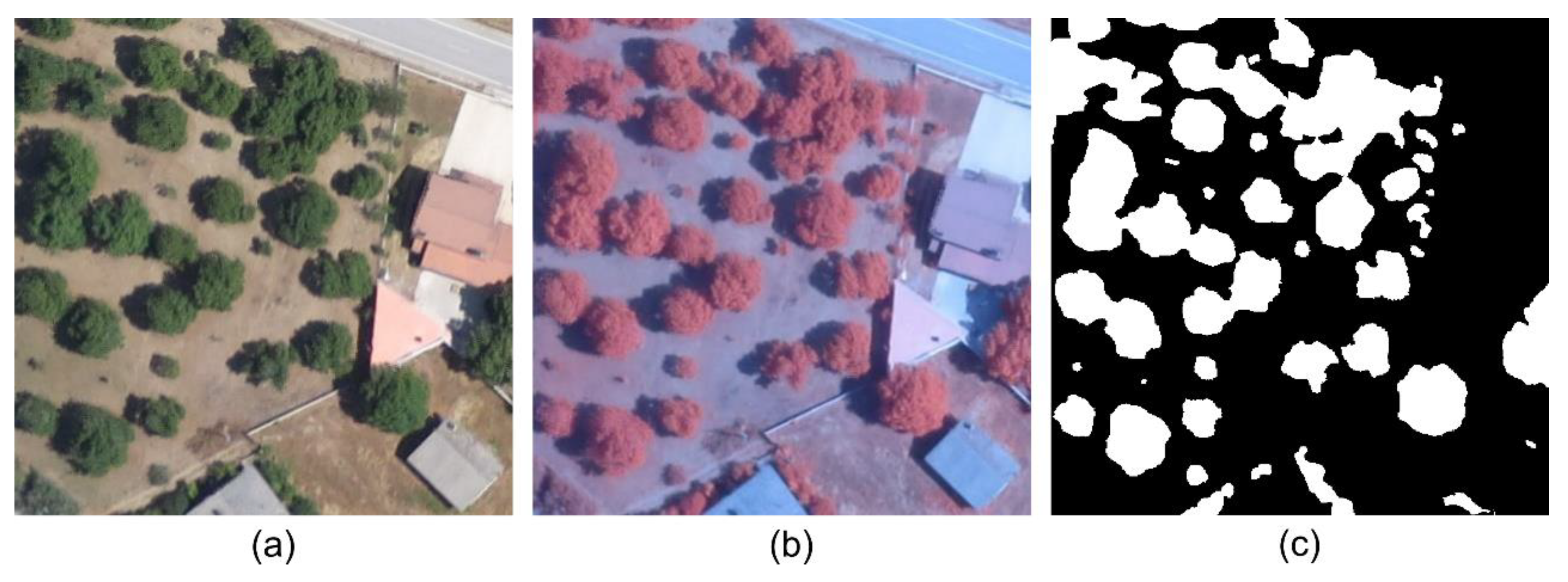
To evaluate these approaches, the area presented in Figure A1 was selected as reference. This area was selected based on the existence of other features than vegetation, as infrastructures, such as houses with different roofs, roads, bare soil, and shadows casted by trees canopy.
Figure A1.
Reference area used for the evaluation of the different segmentation approaches: (a) the RGB image; (b) colour infrared image; and (c) manually segmented image.
Figure A1.
Reference area used for the evaluation of the different segmentation approaches: (a) the RGB image; (b) colour infrared image; and (c) manually segmented image.

Otsu’s method is a simple global thresholding technique. It assumes that the image contains two-pixel classes following a bi-modal histogram: one class is composed by the background pixels—corresponding, in this case, to non-vegetated areas—and the other class is composed by foreground pixels, corresponding to vegetation. In this evaluation the method was directly applied to the greyscale images of the RGB and CIR images obtaining a binary image after the method application. The adaptive thresholding technique differs from the Otsu’s method in the number of used thresholds T. Whereas Otsu’s method is globally applied to the image, this approach applies different thresholds to sub-regions of the image. Similarly, to the Otsu’s method, this technique was applied to the RGB and CIR grayscale images, resulting in a binary image. K-means clustering is a non-supervised method that groups pixels in a K number of clusters in accordance with their likelihood. In this case the method was applied to the RGB and CIR images of the selected area and K was set to two, i.e., it was intended to divide the image into two distinct clusters, one representing vegetation and other non-vegetation, the vegetation cluster was then binarized for comparison against the manually segmented image. HSV is a colour space composed by Hue, Saturation and Value (or Bright), instead of the commonly used RGB colour space. This way, both RGB and CIR images were converted to HSV colour space, and the Hue band was used, it contains colour information, its thresholding was based in upper and lower limits, Hue values differ from zero to one, the values used for the RGB image were between 0.2 to 0.27, corresponding to the green colour, whereas, in the CIR case, as vegetation assumes a magenta colour the selected values where located between 0.85 to 1. The values within these ranges were then binarized (set to one) whereas other values where considered as background (set to zero). The last evaluated approach, which is commonly found in studies dealing with vegetation segmentation, is the usage of VI. This way, two different VI were applied, the RGBVI to the RGB image and the ExRE to the CIR imagery, these VIs were selected based in the results from the VI selection, see Appendix B for more information. To segment the vegetation the Otsu’s method was applied to resulting VI images.
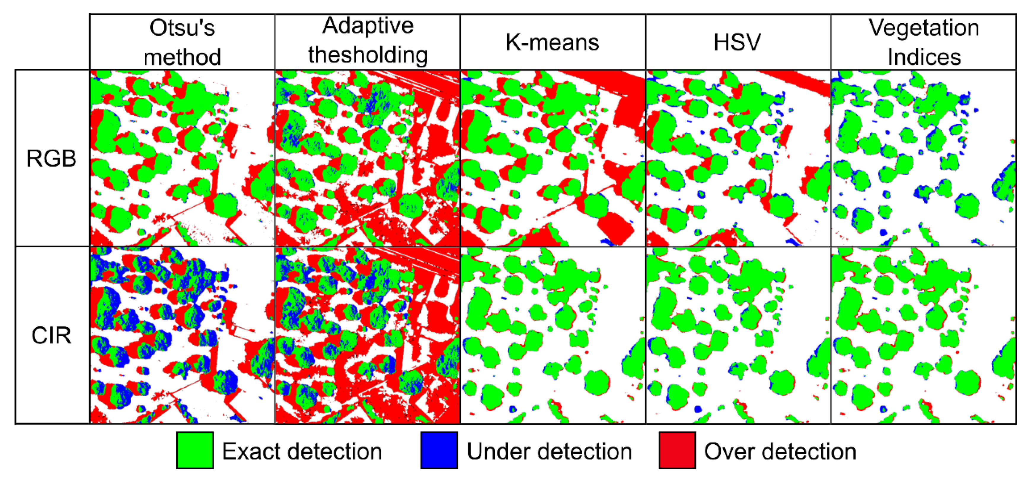
The evaluation of the different approaches was based in a pixel-wise comparison against the manually segmented image (Figure A1c), and three classes were considered, exact detection, over detection and under detection. The obtained results applied to the RGB and CIR images from the reference scene are shown in Figure A2.
Figure A2.
Results obtained from the different segmentation approaches of the same area for the RGB and colour infrared (CIR) images. Exact detection of vegetation areas represented in green and exact detection of non-vegetation areas represented in black; red represents over detection; and blue signals under detection.

Table A1 presents the percentage of exact, over and under detection, for each evaluated approach in the two tested images. According to the obtained results it is possible to conclude that K-means had a good performance in the CIR image with an exact detection rate of 96%. However, when applied to the RGB image this rate decreases to 74% with an over detection of 25%. The over detection mainly corresponds to infrastructures and shadows, being this approach not ideal to apply for vegetation detection in RGB images. As for the results obtained for the segmentation approach based in the Otsu’s method, obtained a high over detection rate in the CIR image (18%), the same was verified for the under detection (17%). When analysing the results obtained from the RGB image the over detection rate decreases to 2%, however the under detection remains with a considerable percentage (16%). The adaptive thresholding approach did not provide satisfactory results for both images, the method obtained error rates higher than 40%. This is due to the method not being capable to discriminate between shadows and infrastructures from the vegetation since it is based in local threshold values. In what concerns the results obtained from the HSV-based technique, the results were acceptable in both tested images. The HSV conversion of the CIR image, showed an exact detection of 96%, although, in the case of the RGB image it decreased to 84%, being this a considerably acceptable value. However, the former, suffers from the same problem as other approaches, some outliers were wrongly classified (shadows and roads). The good detection accuracy in K-means and HSV-based techniques in CIR imagery can be explained due to the high reflection of the RedEdge in the vegetation, contributing for a clearer vegetation discrimination. The VI-based approach obtained the best overall results, with exact detection rates greater than 93%, being this value higher in the CIR image (96%), still the accuracy obtained in the RGB image was satisfactory (93%).

Table A1.
Results of the performance of the different methods classified in exact, over and under detection when compared to the manually segmented image of the same area for the RGB and colour infrared (CIR) images.
Table A1.
Results of the performance of the different methods classified in exact, over and under detection when compared to the manually segmented image of the same area for the RGB and colour infrared (CIR) images.
| Method | Image Type | Exact Detection (%) | Over Detection (%) | Under Detection (%) |
|---|---|---|---|---|
| Otsu | RGB | 82 | 16 | 2 |
| CIR | 65 | 18 | 17 | |
| Adaptive threshold | RGB | 59 | 38 | 3 |
| CIR | 45 | 46 | 9 | |
| K-means | RGB | 74 | 25 | 1 |
| CIR | 96 | 3 | 1 | |
| HSV | RGB | 84 | 13 | 3 |
| CIR | 96 | 2 | 2 | |
| Vegetation index | RGB | 93 | 1 | 6 |
| CIR | 96 | 3 | 1 |
This way, when comparing the results of all approaches tested for vegetation segmentation the one based in VI was the one with the best overall performance for both types of images (94.5% mean value). The two evaluated thresholding methods (Otsu’s and adaptive) were the approaches with lower exact detection accuracy with, respectively, 73.5% and 52% mean accuracy in vegetation detection. However, with image processing these methods provide more accuracy, as de case of the VI-based approach were the Otsu’s method is applied to the images driven from the VI computation. The K-means and HSV-based segmentation approaches reached a reliable performance in the CIR image, which can be explained by the difference caused by the RE band where vegetation has higher pixel values, although when to the RGB image their performance decreases, their overall accuracy is 85% and 90%, respectively. Thus, the VI-based approach, more specifically using ExRE for CIR imagery and RGBVI in the case of RGB images (see Appendix B), corresponded to the selected approach for vegetation segmentation, since it had better behaviour, in both CIR and RGB images, thus providing a flexible and robust approach with respect to the type of image being used, with low error rates. These results motivated the selection of the VI-based approach for vegetation segmentation procedure of the method proposed in this study.
Appendix B
To select the most suitable VI, a study was accomplished using the 17 VIs listed in Table A2): six based exclusively on RGB bands and 11 VIs based on RGB and NIR/RE band combinations. These VIs were chosen due to their potential relevance in vegetation segmentation (highlighting vegetation areas). The validation was performed in the different areas, in the three epochs, presented in Figure 9 (see location in Figure 1), selected to be representative: recent chestnut plantations, adult chestnut trees and both types, were included. The proximity between chestnut trees was also considered in the areas’ selection: plantations with regular space between trees and trees with overlapping canopy areas. These areas were used as input of the proposed method and the first two phases of method’s step one were performed (VI application and image thresholding). Results provided by the application of the VI-based segmentation (binary images) were compared with manual segmentation. To evaluate the segmentation accuracy, false negative and false positive rates of image pixels were calculated. False negatives are defined as vegetation pixels that were classified as background pixels (under detection). False positives are defined as background pixels that were classified as vegetation (over detection).
Over detection values correspond to false positives, i.e., values detected as vegetation but that are not classified as vegetation in the manual segmentation; and under detection values that correspond to false negatives, i.e., values that were classified as vegetation in the manual segmentation but were not detected as such by the applied VI.
Table A2.
List of broadband vegetation indices implemented and tested in the proposed method.
| Vegetation Indices Requiring NIR and RGB Bands | ||
| Name | Equation | Reference |
| Blue Normalized Difference Vegetation Index | Hancock and Dougherty [48] | |
| Difference Vegetation Index | Tucker [49] | |
| Enhanced Vegetation Index | Justice et al. [50] | |
| Excess RedEdge | Proposed in this study, derived from ExG | |
| Green Difference Vegetation Index | Sripada et al. [51] | |
| Green Normalized Difference Vegetation Index | Gitelson et al. [52] | |
| Green Soil-Adjusted Vegetation Index | Sripada et al. [51] | |
| Modified Soil-Adjusted Vegetation Index | Qi et al. [53] | |
| Normalized Difference Vegetation Index | Rouse et al. [54] | |
| Optimized Soil-Adjusted Vegetation Index | Rondeaux et al. [55] | |
| Soil-Adjusted Vegetation Index | Huete [56] | |
| Vegetation Indices Requiring only RGB Bands | ||
| Name | Equation | Reference |
| Excess Green | Woebbecke et al. [57] | |
| Green-Blue Vegetation Index | Kawashima and Nakatani [58] | |
| Green-Red Vegetation Index | Tucker [49] | |
| Modified Green Red Vegetation Index | Bendig et al. [59] | |
| Red Green Blue Vegetation Index | Bendig et al. [59] | |
| Vegetation Index Green | Gitelson et al. [60] | |
where, the reflectance values of each band is represented by R: Red; G; Green; B: Blue; N: NIR; and .
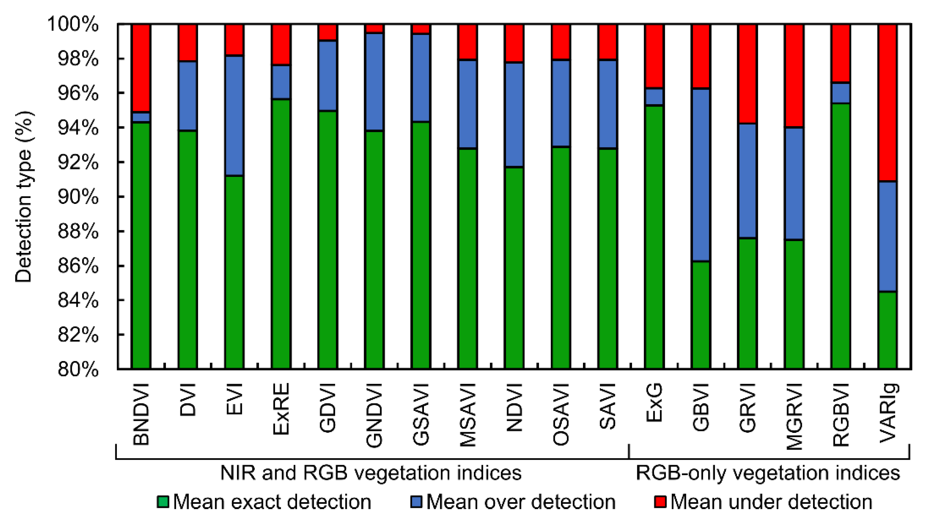
Figure A3 presents the mean results of the performed validation, using the VIs listed in Table A2. For a complete overview, the results are presented, per tested area, in Table A3 which shows the exact detection percentage.
Figure A3.
Mean accuracy of exact, over and under detection in the evaluated vegetation indices from the comparison with manual segmentation masks from the seven evaluated areas.
Figure A3.
Mean accuracy of exact, over and under detection in the evaluated vegetation indices from the comparison with manual segmentation masks from the seven evaluated areas.

Table A3.
Mean near-infrared (NIR) and RGB vegetation indices (VI) exact, over and under detection percentages for the evaluated chestnut plantations in epoch (year).
Table A3.
Mean near-infrared (NIR) and RGB vegetation indices (VI) exact, over and under detection percentages for the evaluated chestnut plantations in epoch (year).
| VI | 2014 | 2015 | 2017 | ||||||
|---|---|---|---|---|---|---|---|---|---|
| Exact (%) | Over (%) | Under (%) | Exact (%) | Over (%) | Under (%) | Exact (%) | Over (%) | Under (%) | |
| Vegetation Indices Requiring NIR and RGB Bands | |||||||||
| BNDVI | 94.9% | 0.8% | 4.3% | 94.4% | 0.2% | 5.4% | 93.7% | 0.7% | 5.6% |
| DVI | 94.2% | 3.7% | 2.1% | 92.8% | 4.8% | 2.4% | 94.4% | 3.6% | 2.0% |
| EVI | 92.1% | 6.1% | 1.7% | 89.9% | 7.8% | 2.3% | 91.6% | 6.9% | 1.4% |
| ExRE | 95.8% | 2.1% | 2.1% | 95.9% | 1.3% | 2.9% | 95.3% | 2.5% | 2.2% |
| GDVI | 94.7% | 4.4% | 0.8% | 95.8% | 2.9% | 1.3% | 94.3% | 4.9% | 0.8% |
| GNDVI | 93.8% | 5.8% | 0.4% | 95.1% | 4.0% | 0.9% | 92.5% | 7.2% | 0.3% |
| GSAVI | 94.2% | 5.3% | 0.5% | 95.5% | 3.5% | 0.9% | 93.2% | 6.4% | 0.3% |
| MSAVI | 93.5% | 4.5% | 2.0% | 91.8% | 5.8% | 2.4% | 93.1% | 5.1% | 1.7% |
| NDVI | 92.6% | 5.2% | 2.2% | 90.7% | 6.6% | 2.7% | 91.8% | 6.4% | 1.8% |
| OSAVI | 93.5% | 4.4% | 2.0% | 91.9% | 5.7% | 2.4% | 93.3% | 5.0% | 1.7% |
| SAVI | 93.5% | 4.5% | 2.0% | 91.8% | 5.8% | 2.4% | 93.1% | 5.1% | 1.7% |
| Vegetation Indices Requiring only RGB Bands | |||||||||
| ExG | 95.8% | 0.9% | 3.3% | 95.2% | 1.2% | 3.5% | 94.9% | 0.9% | 4.3% |
| GBVI | 88.8% | 8.1% | 3.2% | 80.4% | 16.3% | 3.4% | 89.7% | 5.7% | 4.6% |
| GRVI | 89.5% | 5.1% | 5.4% | 85.5% | 8.6% | 5.9% | 87.7% | 6.2% | 6.0% |
| MGRVI | 89.4% | 5.1% | 5.5% | 85.4% | 8.3% | 6.3% | 87.6% | 6.2% | 6.2% |
| RGBVI | 95.9% | 1.1% | 3.0% | 95.2% | 1.4% | 3.3% | 95.1% | 1.1% | 3.9% |
| VARIg | 87.2% | 5.1% | 7.8% | 81.6% | 7.7% | 10.7% | 84.7% | 6.5% | 8.8% |
The results allow to conclude that, in general, NIR-based VIs presented a better overall performance, mean exact detection of 93% with a standard deviation of 0.7% considering the three flight campaigns. However, the performance achieved by RGB-based VIs presented an accuracy rate close to 90% (standard deviation of 1.6% in the three flight campaigns), if excluding VARIg. If discarding the less performant VIs (exact detection lower than 90%), the overall accuracy rate is around 94%.
The obtained results from the different VI motivated the selection of the ExRE as it was the VI with the best overall performance (mean accuracy of 96%). Despite the selection of ExRE, which is proposed in this study (being an adaptation of ExG to CIR imagery), as the VI of better performance, there were other NIR-based VIs with similar performance (~95%), therefore with equivalent results, namely: GDVI, GNDVI and GSAVI. However, if only RGB images are available, the method maintains its performance. Indeed, ExG and RGBVI reached an overall accuracy around 95%.
References
- Martins, L.; Castro, J.P.; Bento, R.; Sousa, J.J. Monitorização da condição fitossanitária do castanheiro por fotografia aérea obtida com aeronave não tripulada. Rev. Ciências Agrárias 2015, 38, 184–190. [Google Scholar]
- Valverde, A.; González-Tirante, M.; Medina-Sierra, M.; Rivas, R.; Santa-Regina, I.; Igual, J.M. Culturable bacterial diversity from the chestnut (Castanea sativa Mill.) phyllosphere and antagonism against the fungi causing the chestnut blight and ink diseases. AIMS Microbiol. 2017, 3, 293–314. [Google Scholar] [CrossRef]
- Vettraino, A.M.; Morel, O.; Perlerou, C.; Robin, C.; Diamandis, S.; Vannini, A. Occurrence and distribution of Phytophthora species in European chestnut stands, and their association with Ink Disease and crown decline. Eur. J. Plant Pathol. 2005, 111, 169. [Google Scholar] [CrossRef]
- Rigling, D.; Prospero, S. Cryphonectria parasitica, the causal agent of chestnut blight: Invasion history, population biology and disease control. Mol. Plant Pathol. 2018, 19, 7–20. [Google Scholar] [CrossRef]
- Battisti, A.; Benvegnù, I.; Colombari, F.; Haack, R.A. Invasion by the chestnut gall wasp in Italy causes significant yield loss in Castanea sativa nut production. Agric. For. Entomol. 2014, 16, 75–79. [Google Scholar] [CrossRef]
- Portela, E.; Roboredo, M.; Louzada, J. Assessment and Description of Magnesium Deficiencies in Chestnut Groves. J. Plant Nutr. 2003, 26, 503–523. [Google Scholar] [CrossRef]
- Martins, L.; Castro, J.P.; Gouveia, E. Biological control of chestnut blight in Portugal. Acta Hortic. 2014, 1043, 51–56. [Google Scholar] [CrossRef]
- Colomina, I.; Molina, P. Unmanned aerial systems for photogrammetry and remote sensing: A review. ISPRS J. Photogramm. Remote Sens. 2014, 92, 79–97. [Google Scholar] [CrossRef] [Green Version]
- Pádua, L.; Vanko, J.; Hruška, J.; Adão, T.; Sousa, J.J.; Peres, E.; Morais, R. UAS, sensors, and data processing in agroforestry: A review towards practical applications. Int. J. Remote Sens. 2017, 38, 2349–2391. [Google Scholar] [CrossRef]
- Järnstedt, J.; Pekkarinen, A.; Tuominen, S.; Ginzler, C.; Holopainen, M.; Viitala, R. Forest variable estimation using a high-resolution digital surface model. ISPRS J. Photogramm. Remote Sens. 2012, 74, 78–84. [Google Scholar] [CrossRef]
- Zarco-Tejada, P.J.; Diaz-Varela, R.; Angileri, V.; Loudjani, P. Tree height quantification using very high resolution imagery acquired from an unmanned aerial vehicle (UAV) and automatic 3D photo-reconstruction methods. Eur. J. Agron. 2014, 55, 89–99. [Google Scholar] [CrossRef] [Green Version]
- Mohan, M.; Silva, C.A.; Klauberg, C.; Jat, P.; Catts, G.; Cardil, A.; Hudak, A.T.; Dia, M. Individual Tree Detection from Unmanned Aerial Vehicle (UAV) Derived Canopy Height Model in an Open Canopy Mixed Conifer Forest. Forests 2017, 8, 340. [Google Scholar] [CrossRef]
- Zhen, Z.; Quackenbush, L.J.; Zhang, L. Trends in Automatic Individual Tree Crown Detection and Delineation—Evolution of LiDAR Data. Remote Sens. 2016, 8, 333. [Google Scholar] [CrossRef]
- Lindberg, E.; Holmgren, J. Individual Tree Crown Methods for 3D Data from Remote Sensing. Curr. For. Rep. 2017, 3, 19–31. [Google Scholar] [CrossRef] [Green Version]
- Wallace, L.; Lucieer, A.; Watson, C.S. Evaluating Tree Detection and Segmentation Routines on Very High Resolution UAV LiDAR Data. IEEE Trans. Geosci. Remote Sens. 2014, 52, 7619–7628. [Google Scholar] [CrossRef]
- Liu, T.; Im, J.; Quackenbush, L.J. A novel transferable individual tree crown delineation model based on Fishing Net Dragging and boundary classification. ISPRS J. Photogramm. Remote Sens. 2015, 110, 34–47. [Google Scholar] [CrossRef]
- Eysn, L.; Hollaus, M.; Lindberg, E.; Berger, F.; Monnet, J.-M.; Dalponte, M.; Kobal, M.; Pellegrini, M.; Lingua, E.; Mongus, D.; et al. A Benchmark of Lidar-Based Single Tree Detection Methods Using Heterogeneous Forest Data from the Alpine Space. Forests 2015, 6, 1721–1747. [Google Scholar] [CrossRef] [Green Version]
- Ok, A.O.; Ozdarici-Ok, A. 2-D delineation of individual citrus trees from UAV-based dense photogrammetric surface models. Int. J. Digit. Earth 2018, 11, 583–608. [Google Scholar] [CrossRef]
- Pádua, L.; Hruška, J.; Bessa, J.; Adão, T.; Martins, L.M.; Gonçalves, J.A.; Peres, E.; Sousa, A.M.R.; Castro, J.P.; Sousa, J.J. Multi-Temporal Analysis of Forestry and Coastal Environments Using UASs. Remote Sens. 2017, 10, 24. [Google Scholar] [CrossRef]
- Instituto Nacional de Estatística, I.P. Estatísticas Agrícolas 2016; Instituto Nacional de Estatística, I.P.: Lisbon, Portugal, 2017; ISBN 978-989-25-0395-0. [Google Scholar]
- Borges, O.; Gonçalves, B.; de Carvalho, J.L.S.; Correia, P.; Silva, A.P. Nutritional quality of chestnut (Castanea sativa Mill.) cultivars from Portugal. Food Chem. 2008, 106, 976–984. [Google Scholar] [CrossRef]
- Wang, J.; Ge, Y.; Heuvelink, G.B.M.; Zhou, C.; Brus, D. Effect of the sampling design of ground control points on the geometric correction of remotely sensed imagery. Int. J. Appl. Earth Obs. Geoinf. 2012, 18, 91–100. [Google Scholar] [CrossRef]
- Agüera-Vega, F.; Carvajal-Ramírez, F.; Martínez-Carricondo, P. Assessment of photogrammetric mapping accuracy based on variation ground control points number using unmanned aerial vehicle. Measurement 2017, 98, 221–227. [Google Scholar] [CrossRef]
- Otsu, N. A Threshold Selection Method from Gray-Level Histograms. IEEE Trans. Syst. Man. Cybern. 1979, 9, 62–66. [Google Scholar] [CrossRef]
- Martins, L.M.; Castro, J.P.; Bento, R.; Sousa, J.J. Chestnut health monitoring by aerial photographs obtained by unnamed aerial vehicle. Rev. Ciências Agrárias 2015, 38, 184–190. [Google Scholar]
- Martins, L.; Castro, J.; Macedo, W.; Marques, C.; Abreu, C. Assessment of the spread of chestnut ink disease using remote sensing and geostatistical methods. Eur. J. Plant Pathol. 2007, 119, 159–164. [Google Scholar] [CrossRef]
- Castro, J.; Azevedo, J.C.; Martins, L. Temporal Analysis of Sweet Chestnut Decline in Northeastern Portugal Using Geostatistical Tools. Acta Hortic. 2010, 886, 405–410. [Google Scholar] [CrossRef]
- Martins, L.M.; Lufinha, M.I.; Marques, C.P.; Abreu, C.G. Small format aerial photography to assess chestnut ink disease. For. Snow Landsc. Res. 2001, 73, 357–360. [Google Scholar]
- Martins, L.; Castro, J.; Marques, C.; Abreu, C. Assessment of the Spread of Chestnut Ink Disease from 1995 to 2005 Using Aerial Photography and Geostatistical Methods. Acta Hortic. 2009, 349–354. [Google Scholar] [CrossRef]
- Martins, L.; Castro, J.P.; Macedo, F.; Marques, C.; Abreu, C. Índices espectrais em fotografia aérea de infravermelho próximo na monitorização da doença tinta do castanheiro. In Proceedings of the V Congresso Florestal Nacional, Instituto Politécnico de Viseu, Viseu, Portugal, 16–19 May 2005. [Google Scholar]
- Yin, D.; Wang, L. Individual mangrove tree measurement using UAV-based LiDAR data: Possibilities and challenges. Remote Sens. Environ. 2019, 223, 34–49. [Google Scholar] [CrossRef]
- Pádua, L.; Marques, P.; Adáo, T.; Hruška, J.; Peres, E.; Morais, R.; Sousa, A.; Sousa, J.J. UAS-based Imagery and Photogrammetric Processing for Tree Height and Crown Diameter Extraction. In Proceedings of the International Conference on Geoinformatics and Data Analysis, Prague, Czech Republic, 20–22 April 2018; ACM: New York, NY, USA, 2018; pp. 87–91. [Google Scholar]
- Surový, P.; Ribeiro, N.A.; Panagiotidis, D. Estimation of positions and heights from UAV-sensed imagery in tree plantations in agrosilvopastoral systems. Int. J. Remote Sens. 2018, 39, 4786–4800. [Google Scholar] [CrossRef] [Green Version]
- Assembleia da Républica Regulamento n.o 1093/2016, Diário da República n.o 238/2016, Série II; Imprensa Nacional Casa da Moeda: Lisbon, Portugal, 2016; pp. 36613–36622.
- Panagiotidis, D.; Abdollahnejad, A.; Surový, P.; Chiteculo, V. Determining tree height and crown diameter from high-resolution UAV imagery. Int. J. Remote Sens. 2017, 38, 2392–2410. [Google Scholar] [CrossRef]
- Díaz-Varela, R.A.; de la Rosa, R.; León, L.; Zarco-Tejada, P.J. High-Resolution Airborne UAV Imagery to Assess Olive Tree Crown Parameters Using 3D Photo Reconstruction: Application in Breeding Trials. Remote Sens. 2015, 7, 4213–4232. [Google Scholar] [CrossRef] [Green Version]
- Lim, Y.S.; La, P.H.; Park, J.S.; Lee, M.H.; Pyeon, M.W.; Kim, J.-I. Calculation of Tree Height and Canopy Crown from Drone Images Using Segmentation. J. Korean Soc. Surv. Geod. Photogramm. Cartogr. 2015, 33, 605–614. [Google Scholar] [CrossRef] [Green Version]
- Iizuka, K.; Yonehara, T.; Itoh, M.; Kosugi, Y. Estimating Tree Height and Diameter at Breast Height (DBH) from Digital Surface Models and Orthophotos Obtained with an Unmanned Aerial System for a Japanese Cypress (Chamaecyparis obtusa) Forest. Remote Sens. 2018, 10, 13. [Google Scholar] [CrossRef]
- Guerra-Hernández, J.; Cosenza, D.N.; Rodriguez, L.C.E.; Silva, M.; Tomé, M.; Díaz-Varela, R.A.; González-Ferreiro, E. Comparison of ALS- and UAV(SfM)-derived high-density point clouds for individual tree detection in Eucalyptus plantations. Int. J. Remote Sens. 2018, 39, 5211–5235. [Google Scholar] [CrossRef]
- Hernandez, J.G.; Gonzalez-Ferreiro, E.; Sarmento, A.; Silva, J.; Nunes, A.; Correia, A.C.; Fontes, L.; Tomé, M.; Diaz-Varela, R. Using high resolution UAV imagery to estimate tree variables in Pinus pinea plantation in Portugal. For. Syst. 2016, 25. [Google Scholar] [CrossRef]
- Popescu, S.C.; Wynne, R.H.; Nelson, R.F. Measuring individual tree crown diameter with lidar and assessing its influence on estimating forest volume and biomass. Can. J. Remote Sens. 2003, 29, 564–577. [Google Scholar] [CrossRef]
- Guerra-Hernández, J.; González-Ferreiro, E.; Monleón, V.J.; Faias, S.P.; Tomé, M.; Díaz-Varela, R.A. Use of Multi-Temporal UAV-Derived Imagery for Estimating Individual Tree Growth in Pinus pinea Stands. Forests 2017, 8, 300. [Google Scholar] [CrossRef]
- Michez, A.; Piégay, H.; Lisein, J.; Claessens, H.; Lejeune, P. Classification of riparian forest species and health condition using multi-temporal and hyperspatial imagery from unmanned aerial system. Environ. Monit. Assess. 2016, 188, 146. [Google Scholar] [CrossRef]
- Gómez-Candón, D.; Virlet, N.; Labbé, S.; Jolivot, A.; Regnard, J.-L. Field phenotyping of water stress at tree scale by UAV-sensed imagery: New insights for thermal acquisition and calibration. Precis. Agric. 2016, 17, 786–800. [Google Scholar] [CrossRef]
- Park, S.; Nolan, A.; Ryu, D.; Fuentes, S.; Hernandez, E.; Chung, H.; O’Connell, M. Estimation of crop water stress in a nectarine orchard using high-resolution imagery from unmanned aerial vehicle (UAV). In Proceedings of the 21st International Congress on Modelling and Simulation, Gold Coast, Australia, 29 November–4 December 2015; Weber, T., McPhee, M.J., Anderssen, R.S., Eds.; Modelling and Simulation Society of Australia and New Zealand: Canberra, Australia, 2015; pp. 1413–1419. [Google Scholar]
- Gago, J.; Douthe, C.; Coopman, R.E.; Gallego, P.P.; Ribas-Carbo, M.; Flexas, J.; Escalona, J.; Medrano, H. UAVs challenge to assess water stress for sustainable agriculture. Agric. Water Manag. 2015, 153, 9–19. [Google Scholar] [CrossRef]
- Matese, A.; Toscano, P.; Di Gennaro, S.F.; Genesio, L.; Vaccari, F.P.; Primicerio, J.; Belli, C.; Zaldei, A.; Bianconi, R.; Gioli, B. Intercomparison of UAV, Aircraft and Satellite Remote Sensing Platforms for Precision Viticulture. Remote Sens. 2015, 7, 2971–2990. [Google Scholar] [CrossRef] [Green Version]
- Hancock, D.W.; Dougherty, C.T. Relationships between Blue- and Red-based Vegetation Indices and Leaf Area and Yield of Alfalfa. Crop Sci. 2007, 47, 2547–2556. [Google Scholar] [CrossRef]
- Tucker, C.J. Red and photographic infrared linear combinations for monitoring vegetation. Remote Sens. Environ. 1979, 8, 127–150. [Google Scholar] [CrossRef] [Green Version]
- Justice, C.O.; Vermote, E.; Townshend, J.R.G.; Defries, R.; Roy, D.P.; Hall, D.K.; Salomonson, V.V.; Privette, J.L.; Riggs, G.; Strahler, A.; et al. The Moderate Resolution Imaging Spectroradiometer (MODIS): Land remote sensing for global change research. IEEE Trans. Geosci. Remote Sens. 1998, 36, 1228–1249. [Google Scholar] [CrossRef]
- Sripada, R.P.; Heiniger, R.W.; White, J.G.; Meijer, A.D. Aerial Color Infrared Photography for Determining Early In-Season Nitrogen Requirements in Corn. Agron. J. 2006, 98, 968–977. [Google Scholar] [CrossRef]
- Gitelson, A.A.; Kaufman, Y.J.; Merzlyak, M.N. Use of a green channel in remote sensing of global vegetation from EOS-MODIS. Remote Sens. Environ. 1996, 58, 289–298. [Google Scholar] [CrossRef]
- Qi, J.; Chehbouni, A.; Huete, A.R.; Kerr, Y.H.; Sorooshian, S. A modified soil adjusted vegetation index. Remote Sens. Environ. 1994, 48, 119–126. [Google Scholar] [CrossRef]
- Rouse, J.W., Jr.; Haas, R.H.; Schell, J.A.; Deering, D.W. Monitoring Vegetation Systems in the Great Plains with Erts. NASA Spec. Publ. 1974, 351, 309. [Google Scholar]
- Rondeaux, G.; Steven, M.; Baret, F. Optimization of soil-adjusted vegetation indices. Remote Sens. Environ. 1996, 55, 95–107. [Google Scholar] [CrossRef]
- Huete, A.R. A soil-adjusted vegetation index (SAVI). Remote Sens. Environ. 1988, 25, 295–309. [Google Scholar] [CrossRef]
- Woebbecke, D.M.; Meyer, G.E.; Von Bargen, K.; Mortensen, D.A. Color indices for weed identification under various soil, residue, and lighting conditions. Trans. ASAE 1995, 38, 259–269. [Google Scholar] [CrossRef]
- Kawashima, S.; Nakatani, M. An Algorithm for Estimating Chlorophyll Content in Leaves Using a Video Camera. Ann. Bot. 1998, 81, 49–54. [Google Scholar] [CrossRef] [Green Version]
- Bendig, J.; Yu, K.; Aasen, H.; Bolten, A.; Bennertz, S.; Broscheit, J.; Gnyp, M.L.; Bareth, G. Combining UAV-based plant height from crop surface models, visible, and near infrared vegetation indices for biomass monitoring in barley. Int. J. Appl. Earth Obs. Geoinf. 2015, 39, 79–87. [Google Scholar] [CrossRef]
- Gitelson, A.A.; Kaufman, Y.J.; Stark, R.; Rundquist, D. Novel algorithms for remote estimation of vegetation fraction. Remote Sens. Environ. 2002, 80, 76–87. [Google Scholar] [CrossRef] [Green Version]
Figure 1.
General overview of the surveyed area: (a) colour infrared (CIR) orthophoto mosaic computed using data from the flight conducted on July 10, 2017; (b) complex area used for vegetation coverage validation; and, (c) chestnut plantations used for tree height and tree crown diameter validation. Coordinates in WGS84 (EPSG:4326).

Figure 2.
Differences in the dense point clouds generated from data of each sensor: (a) RGB; (b) colour infrared; and, (c) combination of both. Example of areas that benefited from the merging process are highlighted.
Figure 2.
Differences in the dense point clouds generated from data of each sensor: (a) RGB; (b) colour infrared; and, (c) combination of both. Example of areas that benefited from the merging process are highlighted.

Figure 3.
Computation of the canopy height model (CHM) obtained from the digital terrain model (DTM) and digital surface model (DSM): (a) profile line upon four chestnut trees; (b) DTM and DSM profiles; and, (c) resulting CHM profile line computed from the subtraction between the DTM and the DSM.
Figure 3.
Computation of the canopy height model (CHM) obtained from the digital terrain model (DTM) and digital surface model (DSM): (a) profile line upon four chestnut trees; (b) DTM and DSM profiles; and, (c) resulting CHM profile line computed from the subtraction between the DTM and the DSM.

Figure 4.
Example of an artificial ground control point (GCP) measuring 100 × 100 cm: (a) being surveyed with a global navigation satellite system (GNSS) receiver placed in the middle of the marker, (b) aerial image taken by the unmanned aerial vehicle. In the left, RGB representation, and in the right, colour infrared representation.

Figure 5.
Proposed method general flow chart.

Figure 6.
Segmentation and first clustering: (a) the original colour infrared image; (b) colour-coded image resulting from the application of ExRE vegetation index; (c) binary image resulting from both the threshold and morphological operations; and, (d) clusters including connected trees highlighted in red.

Figure 7.
Cluster isolation operation applied to an entire chestnut plantation: (a) clusters with area higher than the reference area value, highlighted in red; (b) eroded image; (c) skeleton by zone of influence boundaries, in red, on top of the eroded image; and, (d) image with the separated clusters highlighted in red.

Figure 8.
Cluster isolation process: (a) original cluster composed by five connected chestnut trees; (b) clusters resulting from the morphological erosion operation represented with their centroids; and, (c) effect of the thickening morphological operation, resulting in five unconnected clusters.
Figure 8.
Cluster isolation process: (a) original cluster composed by five connected chestnut trees; (b) clusters resulting from the morphological erosion operation represented with their centroids; and, (c) effect of the thickening morphological operation, resulting in five unconnected clusters.

Figure 9.
Chestnut plantations used for validation: (a) Plantation #1; (b) Plantation #2; (c) Plantation #3; and, (d) Plantation #4. Black lines represent the boarder of the plantation. Coordinates in WGS84 (EPSG:4326).
Figure 9.
Chestnut plantations used for validation: (a) Plantation #1; (b) Plantation #2; (c) Plantation #3; and, (d) Plantation #4. Black lines represent the boarder of the plantation. Coordinates in WGS84 (EPSG:4326).

Figure 10.
Validation of the vegetation coverage area by comparing the automatic binary mask, in an uncontrolled environment, produced by the proposed method, with the reference mask, represented in three colours, overlaid in the orthophoto mosaic, in the left. In the right, contours of the detected trees of the area marked in the dashed polygon. Coordinates in WGS84 (EPSG:4326).

Figure 11.
Validation of the vegetation coverage area by comparison of the automatic binary mask, produced by the proposed method, in four chestnut plantations, with the reference mask, represented in three colours: (a) Plantation 1; (b) Plantation 2; (c) Plantation 3; and, (d) Plantation 4. Left represents 2014; centre 2015, and in the right 2017. Percentage and area of exact, over and under detection are also presented. Coordinates in WGS84 (EPSG:4326).

Figure 12.
Trees’ height estimation validation: comparison between the trees’ height retrieved by the proposed method and those measured in-field using a: (a) 16 cm GSD data and (b) 3 cm GSD data.
Figure 12.
Trees’ height estimation validation: comparison between the trees’ height retrieved by the proposed method and those measured in-field using a: (a) 16 cm GSD data and (b) 3 cm GSD data.

Figure 13.
Trees’ diameter validation: comparison between the in-field measurements by the diameter values estimated by the proposed method: (a) 16 cm GSD data and (b) 3 cm GSD data.
Figure 13.
Trees’ diameter validation: comparison between the in-field measurements by the diameter values estimated by the proposed method: (a) 16 cm GSD data and (b) 3 cm GSD data.

Figure 14.
Multi-temporal analysis between three different periods: (a) Plantation 1; (b) Plantation 2; (c) Plantation 3; and, (d) Plantation 4. Left represents 2014 to 2015; centre 2015 to 2017; and, in the right 2014 to 2017.
Figure 14.
Multi-temporal analysis between three different periods: (a) Plantation 1; (b) Plantation 2; (c) Plantation 3; and, (d) Plantation 4. Left represents 2014 to 2015; centre 2015 to 2017; and, in the right 2014 to 2017.

Figure 15.
Missing trees, new trees and trees with potential phytosanitary problems detected in the multi-temporal analysis of the chestnut plantations and the period when the detection occurred: (a) Plantation 1; (b) Plantation 2; (c) Plantation 3; and (d) Plantation 4; and, (e) example of a tree affected by ink disease from plantation 2.

Figure 16.
Multi-temporal analysis at the individual tree-level: (a) RGB image from 2014 campaign; (b) RGB image from 2017; and, (c) difference mask retrieved by the application of the proposed method.
Figure 16.
Multi-temporal analysis at the individual tree-level: (a) RGB image from 2014 campaign; (b) RGB image from 2017; and, (c) difference mask retrieved by the application of the proposed method.

Table 1.
Flight campaigns (2014, 2015, 2017) characteristics and analysis results. UAV: unmanned aerial vehicle; GSD: ground sample distance.
Table 1.
Flight campaigns (2014, 2015, 2017) characteristics and analysis results. UAV: unmanned aerial vehicle; GSD: ground sample distance.
| Date | UAV | Sensor and Resolution | Overlap (%) (front/side) | GSD (cm) | # Images | Area Covered (ha) |
|---|---|---|---|---|---|---|
| 19 June 2014 | Sensefly eBee | RGB: Canon IXUS 12 7 HS (16.1 MP) CIR: Canon PowerShot ELPH 110 HS (16.1 MP) | 75/60 | 16.21 | 85 RGB 85 CIR | 490 |
| 08 September 2015 | 14.99 | 92 RGB 90 CIR | 436 | |||
| 10 July 2017 | 16.2 | 86 RGB 84 CIR | 517 |
Table 2.
Geometric quality of the orthophoto mosaics used in the multi-temporal analysis.
| Orthophoto Mosaics Compared | N. Checkpoints | RMSE (px) | RMSE (cm) | Standard Deviation (px) | Mean of Residuals (px) | Min/max Residuals (px) |
|---|---|---|---|---|---|---|
| 2014–2015 | 20 | 0.61 | 9.94 | 0.25 | 0.06 | −0.93/1.28 |
| 2014–2017 | 0.90 | 14.44 | 0.38 | 0.10 | −1.12/1.82 | |
| 2015–2017 | 0.71 | 11.38 | 0.32 | −0.04 | −1.36/1.03 |
Table 3.
Chestnut trees vegetation coverage results for the bigger and complex area in 2017 epoch and in four plantations (P#epoch) for the three epochs (2014, 2015, and 2017). Area of true and false positives (TP/FP) and true and false negatives (TN/FN), in m2 along with producer’s accuracy (PA) and user’s accuracy (UA) for chestnut vegetation, and overall accuracy (OA) percentage values. Mean values for the plantation in all parameters are also presented.
| Area/Plantation | TP (m2) | FP (m2) | FN (m2) | TN (m2) | UA (%) | PA (%) | OA (%) |
|---|---|---|---|---|---|---|---|
| Complex area | 107610 | 14698 | 12687 | 346582 | 89.45 | 87.98 | 94.31 |
| P114 | 4951 | 246 | 365 | 9630 | 93.13 | 95.27 | 95.97 |
| P115 | 5096 | 425 | 366 | 9305 | 93.30 | 92.30 | 94.79 |
| P117 | 5248 | 187 | 752 | 9004 | 87.47 | 96.55 | 93.82 |
| P214 | 3460 | 415 | 186 | 6355 | 94.91 | 89.28 | 94.23 |
| P215 | 3632 | 471 | 161 | 6152 | 95.77 | 88.51 | 93.93 |
| P217 | 3929 | 446 | 262 | 5780 | 93.75 | 89.80 | 93.20 |
| P314 | 554 | 57 | 33 | 2033 | 94.42 | 90.62 | 96.64 |
| P315 | 569 | 75 | 55 | 1977 | 91.20 | 88.31 | 95.13 |
| P317 | 719 | 149 | 36 | 1773 | 95.25 | 82.84 | 93.09 |
| P414 | 780 | 44 | 147 | 11645 | 84.15 | 94.66 | 98.49 |
| P415 | 1216 | 99 | 299 | 11002 | 80.28 | 92.45 | 96.85 |
| P417 | 1648 | 223 | 174 | 10572 | 90.46 | 88.09 | 96.86 |
| Mean of P | 2650 | 236 | 236 | 7102 | 91.17 | 90.72 | 95.25 |
Table 4.
Chestnut trees detection accuracy in four plantations (P#epoch) for the three epochs with number of estimated trees and its detection type.
Table 4.
Chestnut trees detection accuracy in four plantations (P#epoch) for the three epochs with number of estimated trees and its detection type.
| Plantation | Number of Trees | Estimated Trees (Variation) | Detection Type (%) | ||||||
|---|---|---|---|---|---|---|---|---|---|
| Good | Missed | Extra | Over | Under | Larger | Smaller | |||
| P114 | 146 | 145 (−1) | 97.93 | 0.69 | - | - | - | 0.69 | 1.38 |
| P115 | 146 | 147 (+1) | 98.64 | 0.68 | - | 0.68 | - | 0.68 | - |
| P117 | 148 | 147 (−1) | 97.96 | 1.36 | - | 0.68 | - | - | 1.36 |
| P214 | 80 | 80 (0) | 100.00 | - | - | - | - | - | - |
| P215 | 80 | 80 (0) | 97.50 | - | - | - | - | 2.50 | - |
| P217 | 80 | 79 (−1) | 93.67 | 1.27 | - | - | - | 1.27 | 5.06 |
| P314 | 44 | 43 (−1) | 93.02 | - | - | - | 2.33 | - | 4.65 |
| P315 | 43 | 42 (−1) | 85.71 | - | - | - | 2.38 | 4.76 | 7.14 |
| P317 | 44 | 44 (0) | 86.36 | - | - | 2.27 | 2.27 | 6.82 | 2.27 |
| P414 | 91 | 88 (−3) | 89.77 | 3.41 | - | - | - | - | 10.23 |
| P415 | 97 | 89 (−8) | 91.01 | 8.99 | - | - | - | 3.37 | 5.62 |
| P417 | 93 | 90 (−3) | 92.22 | 3.33 | - | - | - | 2.22 | 5.56 |
| Mean detection (%) | 93.65 | 1.64 | - | 0.30 | 0.58 | 1.86 | 3.61 | ||
Table 5.
Multi-temporal analysis at the plantation level for: total chestnut area, chestnut coverage area (CA), and mean values of chestnut trees present at the plantation (height, canopy diameter, and area). Values retrieved from four chestnut plantations in each epoch (P#epoch).
Table 5.
Multi-temporal analysis at the plantation level for: total chestnut area, chestnut coverage area (CA), and mean values of chestnut trees present at the plantation (height, canopy diameter, and area). Values retrieved from four chestnut plantations in each epoch (P#epoch).
| Plantation | Chestnut Area (m2) | Chestnut CA (%) | Mean Tree Height (m) | Mean Tree Diameter (m) | Mean Tree Area (m2) |
|---|---|---|---|---|---|
| P114 | 5197 | 34.2 | 6.2 | 7.0 | 36 |
| P115 | 5521 | 36.3 | 6.0 | 7.2 | 38 |
| P117 | 5436 | 35.8 | 6.7 | 7.4 | 37 |
| P214 | 3876 | 37.2 | 6.6 | 8.1 | 48 |
| P215 | 4104 | 39.4 | 6.7 | 8.5 | 51 |
| P217 | 4375 | 42.0 | 7.1 | 8.6 | 55 |
| P314 | 611 | 22.8 | 3.2 | 4.4 | 14 |
| P315 | 645 | 24.1 | 3.9 | 4.7 | 15 |
| P317 | 868 | 32.4 | 4.2 | 5.3 | 20 |
| P414 | 824 | 6.5 | 4.1 | 3.6 | 9 |
| P415 | 1315 | 10.4 | 4.6 | 4.5 | 15 |
| P417 | 1870 | 14.8 | 5.2 | 5.3 | 21 |
Table 6.
Multi-temporal analysis at the individual tree-level: canopy coverage area (CA), canopy diameter (D), and trees’ height (H) estimation for each tree presented in the studied plantation.
Table 6.
Multi-temporal analysis at the individual tree-level: canopy coverage area (CA), canopy diameter (D), and trees’ height (H) estimation for each tree presented in the studied plantation.
| 2014 | 2015 | 2017 | |||||||
|---|---|---|---|---|---|---|---|---|---|
| ID | CA (m2) | D (m) | H (m) | CA (m2) | D (m) | H (m) | CA (m2) | D (m) | H (m) |
| 1 | 65.7 | 10.1 | 7.2 | 63.9 | 9.5 | 7.4 | 73.1 | 10.2 | 8.1 |
| 2 | 51.8 | 8.9 | 7.2 | 47.1 | 8.2 | 6.6 | 55.4 | 9.1 | 6.4 |
| 3 | 45.4 | 8.4 | 6.4 | 43.3 | 8.1 | 6.8 | 59.1 | 9.3 | 7.1 |
| 4 | 35.2 | 7.7 | 5.6 | 34.7 | 7.2 | 5.5 | 33.7 | 7.1 | 4.0 |
| 5 | 33.7 | 7.4 | 5.6 | 24.7 | 6.4 | 5.5 | 9.2 | 4.8 | 4.8 |
| 6 | 39.2 | 7.3 | 6.3 | 37.2 | 7.2 | 6.0 | 45.5 | 7.9 | 6.8 |
| 7 | 44.3 | 7.8 | 7.0 | 43.0 | 7.9 | 6.8 | 48.7 | 8.2 | 7.2 |
| 8 | 61.9 | 9.5 | 8.2 | 64.5 | 9.8 | 8.4 | 72.1 | 10.1 | 8.4 |
| 9 | 54.9 | 9.2 | 7.4 | 55.4 | 9.5 | 7.5 | 63.7 | 9.5 | 8.1 |
| 10 | 52.1 | 8.3 | 6.7 | 54.1 | 8.9 | 6.9 | 62.5 | 9.2 | 7.7 |
© 2019 by the authors. Licensee MDPI, Basel, Switzerland. This article is an open access article distributed under the terms and conditions of the Creative Commons Attribution (CC BY) license (http://creativecommons.org/licenses/by/4.0/).
Share and Cite
MDPI and ACS Style
Marques, P.; Pádua, L.; Adão, T.; Hruška, J.; Peres, E.; Sousa, A.; Sousa, J.J. UAV-Based Automatic Detection and Monitoring of Chestnut Trees. Remote Sens. 2019, 11, 855. https://doi.org/10.3390/rs11070855
AMA Style
Marques P, Pádua L, Adão T, Hruška J, Peres E, Sousa A, Sousa JJ. UAV-Based Automatic Detection and Monitoring of Chestnut Trees. Remote Sensing. 2019; 11(7):855. https://doi.org/10.3390/rs11070855
Chicago/Turabian StyleMarques, Pedro, Luís Pádua, Telmo Adão, Jonáš Hruška, Emanuel Peres, António Sousa, and Joaquim J. Sousa. 2019. "UAV-Based Automatic Detection and Monitoring of Chestnut Trees" Remote Sensing 11, no. 7: 855. https://doi.org/10.3390/rs11070855
Note that from the first issue of 2016, this journal uses article numbers instead of page numbers. See further details here.