Potential of Modern Photogrammetry Versus Airborne Laser Scanning for Estimating Forest Variables in a Mountain Environment

Abstract

Digital stereo aerial photographs are periodically updated in many countries and offer a viable option for the regular update of information on forest variables. We compared the potential of image-based point clouds derived from three different sets of aerial photographs with airborne laser scanning (ALS) to assess plot-level forest attributes in a mountain environment. The three data types used were (A) high overlapping pan-sharpened (80/60%); (B) high overlapping panchromatic band (80/60%); and (C) standard overlapping pan-sharpened stereo aerial photographs (60/30%). We used height and density metrics at the plot level derived from image-based and ALS point clouds as the explanatory variables and Lorey’s mean height, timber volume, and mean basal area as the response variables. We obtained a RMSE = 8.83%, 29.24% and 35.12% for Lorey’s mean height, volume, and basal area using ALS data, respectively. Similarly, we obtained a RMSE = 9.96%, 31.13%, and 35.99% and RMSE = 11.28%, 31.01%, and 35.66% for Lorey’s mean height, volume and basal area using image-based point clouds derived from pan-sharpened stereo aerial photographs with 80/60% and 60/30% overlapping, respectively. For image-based point clouds derived from a panchromatic band of stereo aerial photographs (80%/60%), we obtained an RMSE = 10.04%, 31.19% and 35.86% for Lorey’s mean height, volume, and basal area, respectively. The overall findings indicated that the performance of image-based point clouds in all cases were as good as ALS. This highlights that in the presence of a highly accurate digital terrain model (DTM) from ALS, image-based point clouds offer a viable option for operational forest management in all countries where stereo aerial photographs are updated on a routine basis.

1. Introduction

Forest management relies on accurate, updated, and spatially detailed information about woody forest resources. Measuring forest heights, basal area, and forest timber volume facilitates forest managers in the context of timber-oriented forest management. The options for measuring forest heights, forest timber volume, and basal area with a full enumeration are achievable for selected stands, but are not applicable as standard methods in forest management inventories for geographically large forest areas due to the limitation of resources and high cost [1]. The traditional concept and solutions in forest management practices is the combination of sample based inventories on a stand level, full assessment, and stand wise expert estimation in the presence or absence of tables and aerial photographs that support efficient estimation [2].

An alternative approach developed and implemented in Switzerland during the 1930s is the permanent sample plot approach [1,3,4], which is nowadays a widely used method for forest management planning in large forest areas. However, the accuracy of the results for forest stands is still limited to statistical estimation based on the sample plots. Integrating remote sensing (RS) with a field sample based forest inventory offers a solution for complementing the statistical results using a wall-to-wall mapping approach for all major forest attributes of the entire geographical forest area, and thus offers a new dimension of information for forest management and forest operations planning.

Among the RS data, the potential of airborne laser scanning (ALS) from research to operations has been effectively and efficiently tested and used in a wide range of applications in the field of forest science [5,6,7,8,9]. Among the remote sensing datasets, ALS is the only active technology that has the capability to examine the entire vertical distribution of the forest canopy structure, i.e., upper layer, middle layer, and the ground forest floor. Digital surface models (DSMs) and digital terrain models (DTMs) can be created from the first and last return of the reflected ALS signals. Canopy height models (CHM) or normalized point clouds can be generated by subtracting the ALS-derived DTM from the DSM and ALS point clouds. Extracted height and density metrics at the plot level, or alone from normalized ALS point clouds and CHM can be used for the assessment of many forest height related parameters using an area-based and individual/single-tree detection approach [5,7]. Many countries have been mapped entirely by ALS campaigns such as Denmark, Switzerland, Germany, and the Netherlands [10]. In some Nordic countries, ALS data have been used operationally in the context of forest management [6,9,11,12]. In countries like Germany, the repetition of ALS data are not desirable for continued forest management due to high costs, but digital stereo aerial photographs are updated periodically by the state survey administrations, which are available to the forest department.

Due to current advancements in the field of modern digital aerial photography, 3D image-based point clouds like ALS can also be produced from digital stereo aerial photographs from which various forest height related information like ALS can be generated [13]. However, image-based point clouds are usually generated toward the outer and middle envelope of the forest canopy and cannot provide information about forest floors in a dense forest canopy condition. Under such conditions, a highly accurate DTM is always needed for the normalization of image-based point cloud elevations to the heights above ground (also called CHM), which can only be obtained from ALS [13]. For Germany, highly accurate ALS based DTMs up to 1 m are available for forested areas. Thus, subtracting a historical ALS-derived DTM (some years before) from recently acquired image-based point clouds or DSM can offer a solution for the normalization of image-based point clouds and CHM generation.

Numerous image-based studies have been reported based on different image matching algorithms as implemented in various software packages for the estimation of forest structure variables using an area based approach [10,14,15,16,17], individual/single-tree detection approach [18,19], and a comparison of semi-individual tree crowns with an area based approach [20]. We used SURE, which is specially designed software to generate image-based point clouds for the estimation of forest variables using an area based approach. One of the essential factors in stereo aerial photography is overlap, which is the amount of area in one photograph covered by another and is expressed as a percentage. Usually, aerial photographic surveys are designed to acquire 60% of forward overlap and 30% lateral overlap. The literature shows that the percentage of image overlap influences the accuracy of the 3D point clouds [10]. At present, two studies are being conducted by Bohlin et al. [10] and Nurminen et al. [21], respectively, by testing the impact of image overlap options on the accuracy of forest variables. However, their study sites seem to be located on a relatively flat terrain. Here, we examine the effect of image overlap options for estimating forest attributes in a mountain environment.

Usually, pan-sharpened stereo aerial photographs have been used for the generation of point clouds and for estimating forest variables. For example, Bohlin et al. [10] used pan-sharpened stereo aerial photographs with ground sample distances (GSD) of 0.12 to 0.48 m for the generation of the DSM and the estimation of forest variables. Similarly, Straub et al. [16], Järnstedt et al. [14], and White et al. [17] used pan-sharpened stereo aerial photographs with a GSD of 0.20 m, 0.25 m, and 0.30 m, respectively, for the generation of image-based point clouds and estimation of forest variables. In addition to pan-sharpened stereo aerial photographs, we evaluated for the first time the potential of the only panchromatic band with GSD = 0.10 m for the generation of point clouds and estimating forest variables.

The primary goal of this study was to assess the potential of image-based point clouds derived from stereo aerial photographs for estimating plot level Lorey’s mean height (LH), timber volume (V), and basal area (G) in a mountain environment and compared the results with ALS data. For 3D image-based point clouds, we tested three different sets of aerial photographs, i.e., high overlapping pan-sharpened with 80/60% overlap, the only high overlapping panchromatic band with 80/60% overlap, and pan-sharpened with the standard 60/30% overlap option versus the ALS 3D point clouds for estimating the plot-level forest attributes in a mountain environment.

2. Materials and Methods

2.1. Study Area and Sample Plots

The study area is part of the state forest in Baden–Württemberg, Germany, located in mountainous terrain. It covers an area of 9.8 km², where 885 ha are productive forest stands, and the elevation of the study area ranges from 527 to 1009 meters above sea level (Figure 1). Picea abies dominates the study test site on 640 ha (57.81%), followed by Abies alba on 122 ha (21.08%), Fagus sylvatica on 80 ha (12.80%), Pinus sylvestris L. on 40 ha (5.78%), and Pseudotsuga menziesii on 2.3 ha (1.01%). Some other species, e.g., Larix decidua (0.3%), Acer pseudoplatanus (0.13%), Sorbus aucuparia (0.13%), Alnus glutinosa (0.1%), and Betula pendula (0.62%) rarely occur.

The establishment of a systematic sample plot grid is one of the basic elements of forest management in the state forests in Baden–Württemberg. The sample plots used in this study were established in the course of such forest management inventory. A total of 449 permanent circular concentric plots in March 2015 were measured by the state forest service of Baden–Württemberg, as shown in Figure 1. Out of the total sample plots, 367 were dominated by coniferous trees, 74 were dominated by deciduous trees, and eight were located in open regeneration areas without solid wood. The inventory sample plots were arranged by a systematic regular grid of 100 m by 200 m (Figure 1). Each sample plot consisted of four concentric circular subplots of 2, 3, 6, and 12 m radii. The trees measured at each circular plot depended on tree threshold diameters at breast heights of 7, 10, 15, and 30 cm, respectively. Tree heights were only measured on a subset of the sample trees, concerning species and stand layer. The heights of the trees without measurement were calculated using height–diameter tariffs, which were adjusted for each plot according to the measured heights. Lorey’s mean height was calculated according to the following equation developed by Lorey [22].

$${\mathrm{Lorey}}^{\prime }\mathbf{s} \mathrm{means} \mathrm{height}=\frac{\mathsf{\Sigma }\mathrm{g}.\mathrm{h}}{\mathsf{\Sigma }\mathrm{g}}$$

(1)

where g is the basal area and h is the tree height.

For the calculation of single tree timber volume, the taper function of Kublin [23] was used. The total timber volume at the plot level in cubic meters per hectare was derived by adding the individual tree timber volumes weighted by the inverse of the corresponding sample plot area. Mean basal area was also calculated by adding the individual tree basal area weighted by the inverse of the relevant sample plot area. Additional information on the statistics of Lorey’s mean height, volume, and basal area from all sample plots are shown in

Table 1. Summary of the statistics of forest attributes.

Summary of the statistics of the forest attributes
	Min	25% percentile	Mean	75% percentile	Max	SD
Lorey’s mean height [m]	0	21.37	25.21	30.16	42.19	7.94
Volume [m 3 ha −1]	0	159.4	323.3	456	1215	211.33
Basal area [m 2 ha −1]	0	13.88	25.38	35.96	95.87	15.34

.

2.2. Remote Sensing Data and Processing

Full waveform ALS was obtained in summer 2015. Details about the flight and other system parameters of ALS data used in the study are shown in

Table 2. Information about the flight and system parameters of airborne laser scanning (ALS).

Parameters	ALS
Flying height	600 m above ground
Field of view (full scan angle)	60 degrees
Strip distance [m]	130 m
Measurement rate	LMS-Q780/400 kHz
Point density	>40/m2
Acquisition date	29.04–04.05.2015
Flying velocity	110 ktn

.

Similarly, the details of the flight and system parameters of the stereo aerial photographs used in the study are shown in

Table 3. Information about the flight and technical characteristics of stereo aerial photographs.

Parameters	Stereo Aerial Photographs
Camera	UltraCamXP
Flying height	1200–1400 m above ground
Image overlap	80%/60% and 60%/30%
Swat width [m]	520 [m]
Acquisition date	17.07–19.07.2014
Spectral bands	blue, green, red and near-infrared/only panchromatic band
Resolution (GSD)	0.1 m
Coordinate System	DHDN/3 Gauss–Krüger

.

2.3. Processing Remote Sensing Data

Image-based point clouds were generated from pan-sharpened high overlap stereo aerial photographs (80/60%), standard overlap stereo aerial photographs (60/30%), and the only panchromatic band of high overlap stereo aerial photographs (80/60%) using SURE photogrammetric software by selecting all of the default parameter settings except for changes to the overlap option. SURE is specially-designed photogrammetric software for the generation of dense and precise 3D point clouds [24]. It is based on SGM, which provides dense image-matching point clouds that correspond to the GSD of the stereo images. Using SGM, first, the color values of the pixels are transformed by using non-parametric senses transformation [25]. Next, SGM performs dense image-matching for every pixel by minimizing the difference of the transformed image in the left and the corresponding pixel in the right image [26]. To erase the poor texture of the forested areas, SGM applies a smoothness constraint, which favors correspondence that produces neighboring points with the same depth. Finally, the difference of the transformed values and the smoothness constraints are combined by the weighted sum, which is minimized with an energy function. The SURE software matches every pixel in the base image with similar pixels along the epipolar line (strip) with the neighboring image, and then computes a multi-image-based spatial intersection [26]. The point clouds obtained by each base image are merged by a median-based fusion to form a grid of an entire project [26].

2.4. Computation of Explanatory Variables

The ALS and the image-based point clouds were normalized by subtracting the ALS derived DTM (1 m spatial resolution) to the height of the point cloud’s elevation above ground. Finally, height percentiles (i.e., h99, h95, h90, h80…, h10), and other height metrics, i.e., the maximum, minimum, and mean height for each plot were calculated. In addition, standard deviation (SD), and the coefficient of variation (CV) were also calculated by taking into account the heterogeneity and variation of the forest canopy height. All of the above-mentioned metrics were derived from the vertical distribution of the point clouds by using a 12-meter radius circle corresponding to the size of the ground sample plots.

We also calculated the canopy volume (CVol), and canopy-cover density (cd) parameters that take into account the horizontal distribution of the canopy structure. For the Cvol and cd metrics, we calculated the canopy height model (CHM) through the subtraction of the ALS based DTM from the image-based DSMs and ALS DSM. To generate the DSM, we selected the maximum option that took the highest point clouds within a pre-specified pixel resolution as a filter and natural neighbor option as an interpolation as implemented in ArcMap. The CVol is the sum of all the heights of 1 × 1 m pixel size covering the total circular 12-meter radius sample plot area. The forest canopy density (cd) was calculated by dividing the number of pixels with heights above 2 m by the total number of pixels within an area of a 12 m radius that corresponded to the size of the ground sample plot. In addition, ten types of other forest canopy cover density metrics (i.e., cd1, cd2, cd3,… cd10) were calculated at sample plot locations followed by the methodology adopted by Næsset [7], Rahlf [27], and Straub [16]. More details about all of the above-mentioned heights, and canopy density metrics were described in detail in our previous work i.e., Ullah et al. [28,29].

2.5. Statistical Methods

For the statistical analysis, we used the 12 m radius field sample plots to extract different metrics/explanatory variables from each of the remote sensing datasets. The generated dataset was then screened for collinearity (>0.7 correlation) between the explanatory variables/metrics derived from the remote sensing datasets. The problem of multicollinearity was solved by calculating the variance inflation factors for each of the variables and sequentially dropping the variables, which were found to be above a pre-specified threshold value (>2) as suggested by Zuur [25]. Then, the variance inflation factor was recalculated and the steps repeated until all values were below the threshold. To calculate the variance inflation factor, we used the CAR package of the R-statistics software [30].

After solving the problem of collinearity, we fit multiple regression models between the independent variables (i.e., height and density metrics), which were extracted from the remote sensing datasets and the dependent variables (i.e., ground measured Lorey’s mean height, timber volume, and basal area) at the sample plot locations. After that, a stepwise method was applied where the explanatory variables were removed by minimizing the Akaike Information Criterion.

For the accuracy assessment, the coefficient of determination (R²), and the absolute and relative root mean square (RMSE) as shown in Equations (1) and (2) were computed using leave-one-out cross-validation (LOOCV). In LOOCV, every single observation was held out as a testing set, and the remaining data were used as a training set. We used R-statistical software [31] for the entire calculation.

$$RMSE \left(LOOCV\right)=\sqrt{\frac{1}{n}{\displaystyle \sum }_{i=1}^n{(yi-\widehat{yi})}^2}$$

(2)

$$RMSE [\%]=\frac{RMSE{ }_{\left(LOOCV\right)}}{\overbrace{y}}\ast 100$$

(3)

where yi is the observed values; $\widehat{\mathit{y}\mathit{l}}$ is the predicted value of LOOCV; $\overbrace{\mathit{y}\mathit{i}}$ is the mean of the observed values; and n is the total number of ground sample plots.

In addition to R² and RMSE, we also calculated bias, and bias% according to Equations (4) and (5).

Bias = sum (predicted – observation)/number of observation

(4)

Bias % = 100 * [sum (predicted – observation)/sum of observation]

(5)

Finally, forest variable maps were produced using the wall-to-wall mapping approach by implementing the prediction function developed from the final most models on the rasterized explanatory variables. The final most variables selected for the prediction of Lorey’s height, forest timber volume, and basal area were generated for a grid area of 20 * 20 m, which is considered to be a suitable mapping unit for the 12 m radius circular ground sample plots, as described by White et al. [32] in the best practice guidelines for generating the forest inventory attributes from the ALS data using an area-based approach.

3. Results

Our results showed that the performance of ALS for estimating the Lorey’s mean height was more accurate than image-based point clouds (

Table 4. Airborne laser scanning and image-based point clouds for estimation of Lorey’s mean height.

Remote Sensing Data	Explanatory Variables	Coefficients	R2	RMSE	RMSE%	Bias	Bias %
ALS	intercept	12.59 ***	0.80	2.22	8.83	0.00	0.00
	h99	0.84 ***
	cd1	–9.51.
Image-based point clouds (80/60%)	intercept	9.39 ***	0.73	2.51	9.96	0.15	0.58
	h99	0.77 ***
	cd2	–4.78 **
Image-based point clouds (60/30%)	intercept	12.83 ***	0.68	2.84	11.28	0.00	0.00
	h99	0.73 ***
	cd2	–7.05 ***
Image-based point clouds (80/60%), Panchromatic bands	intercept	6.95 ***	0.73	2.53	10.04	0.00	0.00
	h99	0.78 ***
	cd2	–2.69 **

Note: R² = coefficients of determination, and (*** p < 0.001, ** p < 0.01, * p < 0.05, and p < 0.1) indicates the level of significance of the t-test.

). Moreover, we only found a small difference in obtaining a higher accuracy by using higher overlapping (80/60%) versus standard overlapping (60/30%) for estimating the Lorey’s mean height. Additionally, we did not find any difference between the overall performances of the image-based point clouds derived from the pan-sharpened versus the panchromatic band of stereo aerial photographs (Table 4). Overall bias obtained from the predicted and observed Lorey’s mean height was negligible, however, for image-based point clouds using higher overlapping (60/80%), the bias was found to be slightly higher (Table 4).

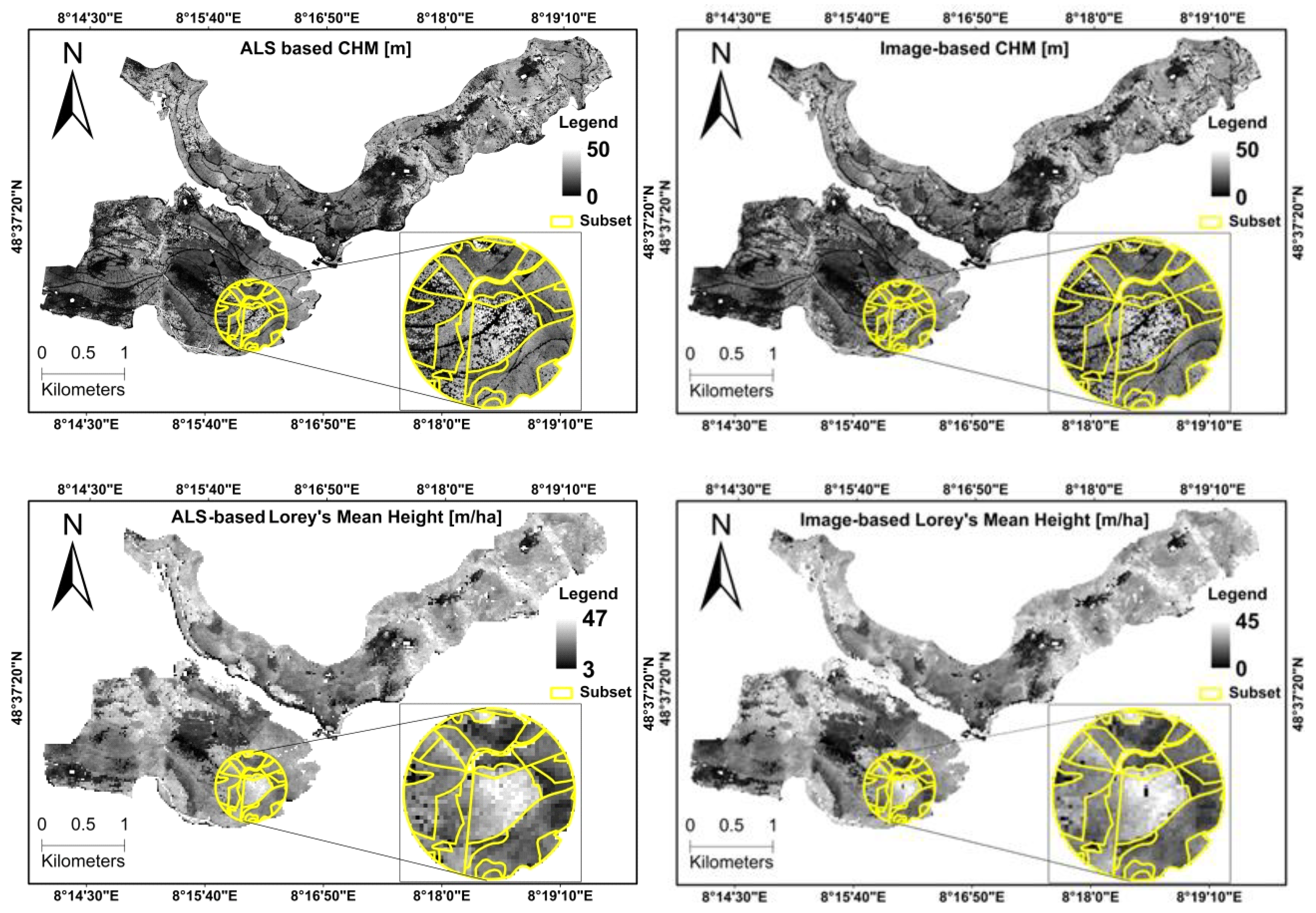
In addition, the scatter plots (Figure 2), and canopy height models of Lorey’s mean height (Figure 3) derived from both the ALS and image-based point clouds did not show any clear difference, thereby confirming our earlier observation.

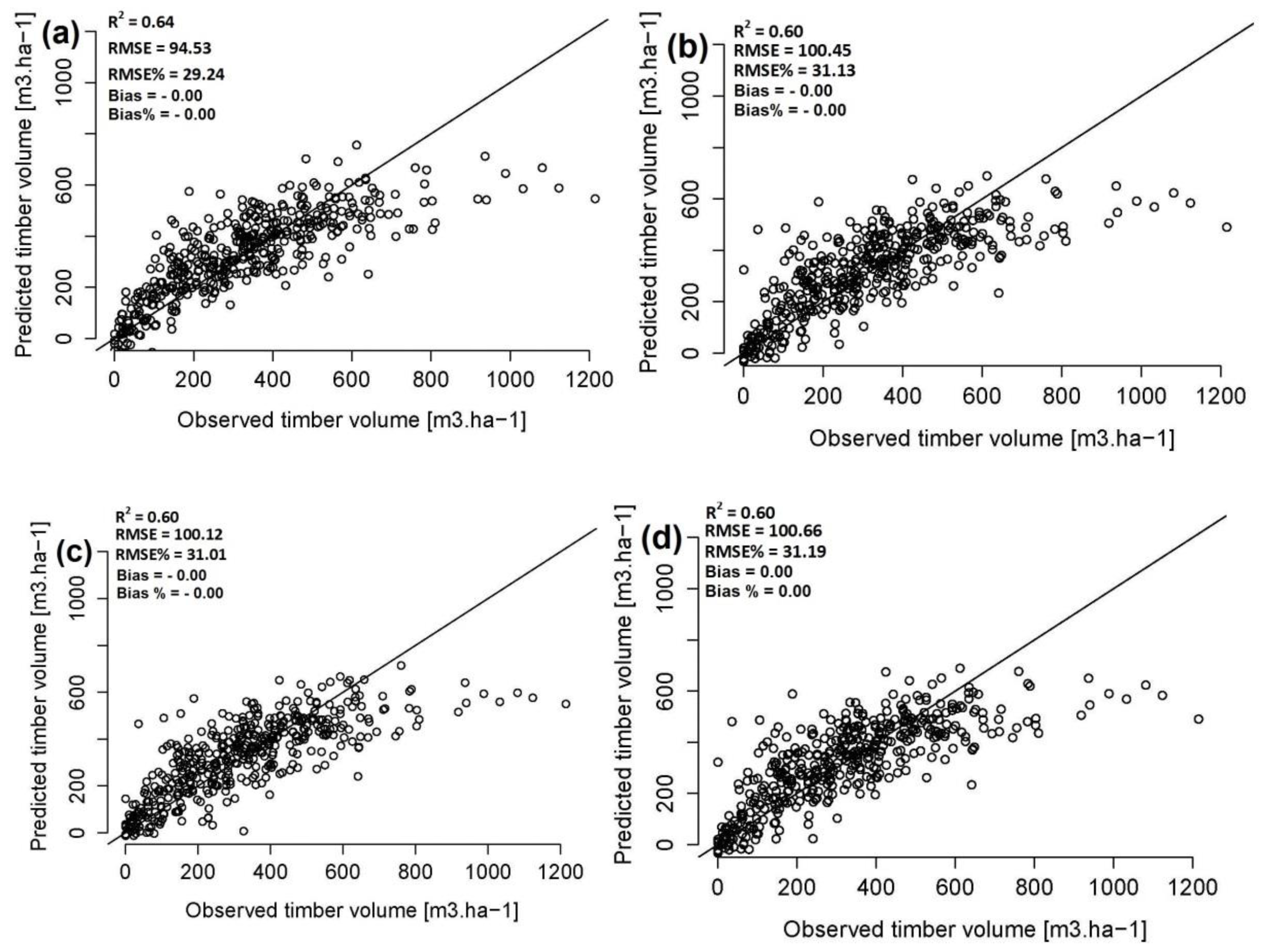
ALS also showed higher accuracy for estimating the forest timber volume than the image-based point clouds by reporting R² and RMSE (

Table 5. Comparison of airborne laser scanning and image-based point clouds for estimating forest timber volume.

Remote Sensing Data	Explanatory Variables	Coefficients	R2	RMSE	RMSE%	Bias	Bias%
ALS	intercept	–1.16	0.64	94.53	29.24	–0.00	–0.00
	h95	14.79 ***
	h30	9.49 ***
	CV	–78.99 ***
Image-based point clouds (80/60%)	intercept	–46.47 **	0.60	100.45	31.13	–0.00	–0.00
	h10	6.20 ***
	h90	14.86 ***
Image-based point clouds (60/30%)	intercept	–28.44.	0.60	100.12	31.01	–0.00	–0.00
	h10	6.40 ***
	h90	13.89
Image-based point clouds (80/60%), Panchromatic bands	Intercept **	–46.55 **	0.60	100.66	31.19	–0.00	–0.00
	h10***	6.18 ***
	h90***	14.86 ***

Note: R² = coefficients of determination, and (*** p < 0.001, ** p < 0.01, * p < 0.05, and p < 0.1) indicates the level of significance of the t-test.

). For the three image-based point clouds, we obtained similar results to estimate the forest timber volume (Table 5). For all four datasets, we obtained a negligible negative bias between the predicted and observed forest timber volume.

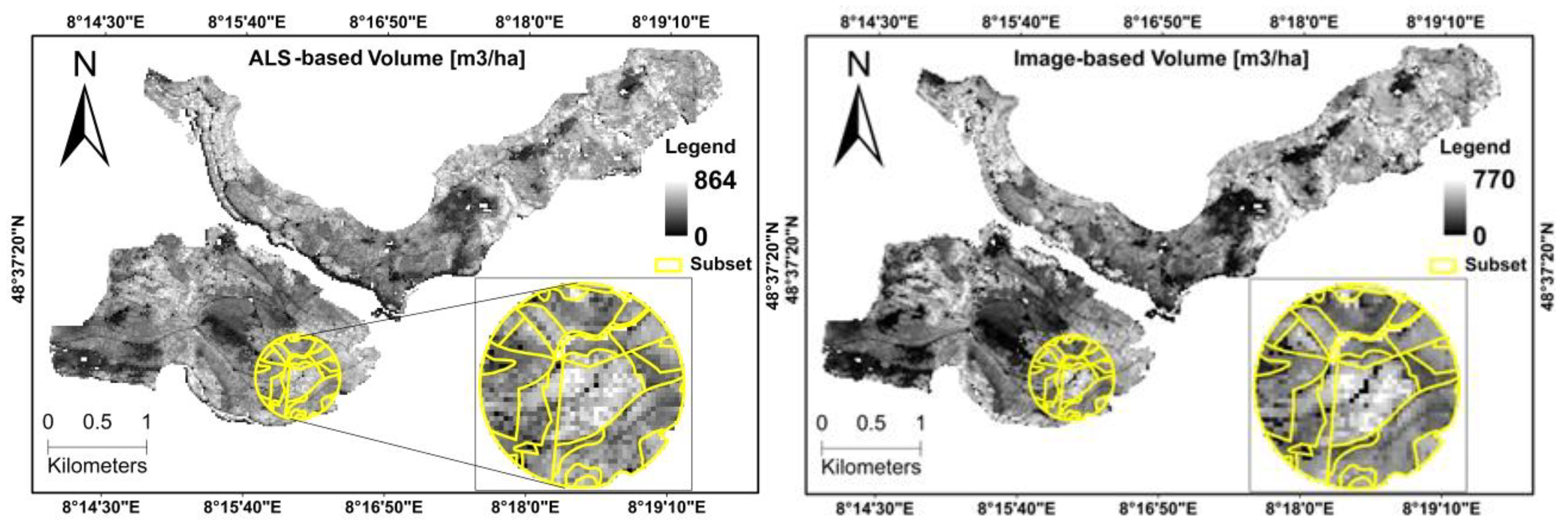
The scatter plots (Figure 4), and forest timber volume maps (Figure 5) derived from both the ALS and image-based point clouds also did not show any clear difference between them. The scatter plots showed that the forest timber volume was overestimated at the lower ranges and underestimated at the higher ranges where the goodness of fit between the predicted and measured forest timber volumes had been plotted (Figure 4).

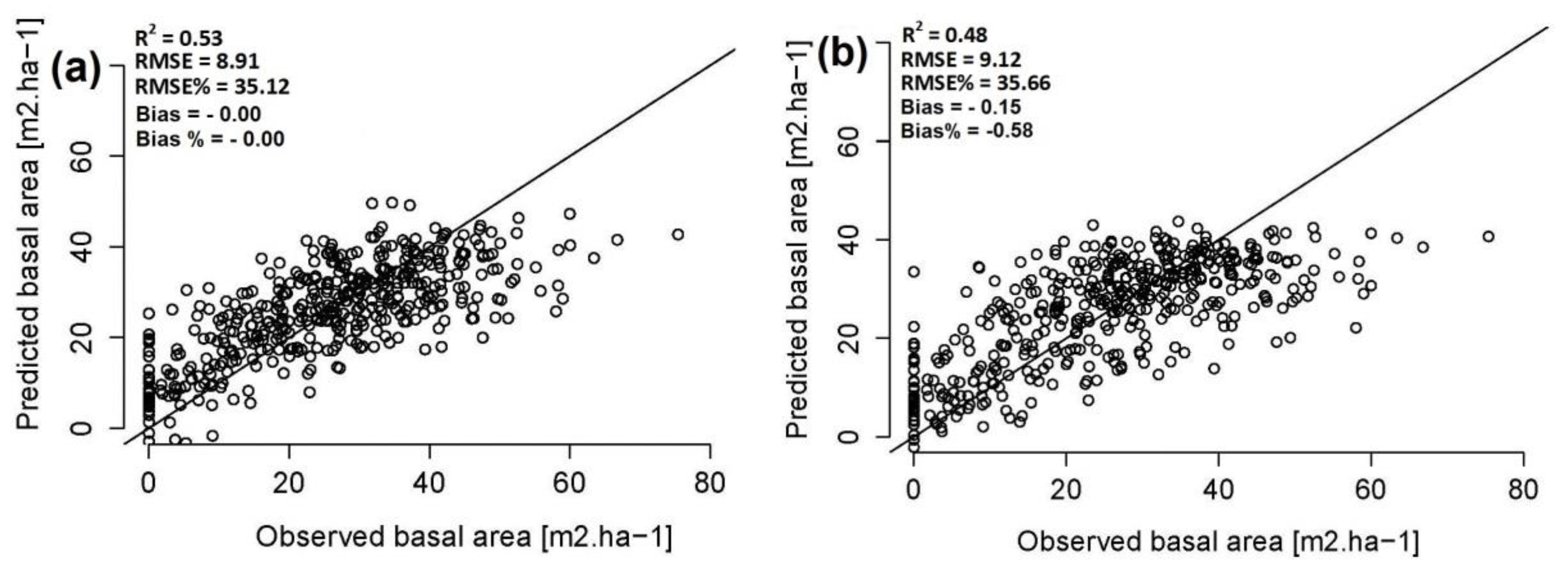
For the prediction of basal area, ALS showed higher accuracy than the three image-based point clouds by reporting R² and RMSE. We did not find any clear difference between the performances of the three image-based point clouds derived from high overlapping (80/60%), standard overlapping (60/30%), and the panchromatic band of the only stereo aerial photographs (80/60%) in estimating the basal area (

Table 6. Comparison of airborne laser scanning and image-based point clouds for estimating basal area.

Remote Sensing Data	Explanatory Variables	Coefficients	R2	RMSE	RMSE%	Bias	Bias%
ALS	intercept	15.20 ***	0.53	8.91	35.12	–0.00	–0.00
	h95	0.64 ***
	h30	0.50 ***
	CV	–14.35 ***
	cd6	7.56 **
Image-based point clouds (80/60%)	intercept	–17.21 ***	0.48	9.12	35.99	–0.15	–0.58
	h80	0.66 ***
	cd	22.75 ***
	cd6	14.57 ***
Image-based point clouds (60/30%)	intercept	–13.53 ***	0.48	9.04	35.66	–0.00	–0.00
	h80	0.69 ***
	cd	20.91 ***
	cd6	10.62 ***
Image-based point clouds (80/60%), Panchromatic bands	intercept	–3.36.	0.48	9.09	35.86	0.00	0.00
	h80	0.68 ***
	cd	8.91 *
	cd6	13.74 ***

Note: R² = coefficients of determination and (*** p < 0.001, ** p < 0.01, * p < 0.05, and p < 0.1) indicates the level of significance of the t-test.

). We found negative negligible bias for ALS, normal overlapping image-based point clouds (60/30%), and positive negligible bias for the only panchromatic band of the higher overlapping image-based point clouds (80/60%), however, for the higher overlapping image-based point (80/60%), the bias was found to be negative and slightly higher between the predicted and the observed basal area.

Likewise, volume in the scatter plots (Figure 6) displaying the basal area was overestimated at the lower ranges and underestimated at the higher ranges where the goodness of fit between predicted and measured basal area was plotted (Figure 7).

4. Discussions

The general aim of this study was to evaluate the potential of ALS and image-based point clouds for estimating forest variables in the context of forest inventories in a mountain environment. As noted above, the performance of ALS was more accurate than the image-based point clouds for estimating Lorey’s mean height, volume, and basal area. However, ALS did not markedly outperform the image-based point clouds by reporting the R², RMSE, and Bias. Several studies have been conducted on the subject of comparison between ALS and image-based point clouds for estimating forest attributes. For instance,

Table 7. Comparison of our findings with other studies.

Forest Inventory Attributes	Järnstedt et al. [14]		White et al. [17]		Our Results
	Image	ALS	Image	ALS	Image	ALS
Mean height	28.23%	18.61%	N/A	N/A	N/A	N/A
Dominant height	18.17%	11.79%	N/A	N/A	N/A	N/A
Lorey’s mean height	N/A	N/A	14%	8.96%	9.96%	8.83%
Basal area	36.23%	27.89%	37.68%	35.38%	31.13%	29.24%
Volume	40.39%	31.26%	36.87%	33.24%	35.99%	35.12%
Diameter	33.67%	25.26%	N/A	N/A	N/A	N/A

shows our findings in comparison with previous studies conducted by White et al. [17], and Järnstedt et al. [14]. Our image-based results were slightly more accurate than the results obtained by White et al. [17] and Järnstedt et al. [14]. This could be due to the software packages, which are based on different methodological approaches for the generation of 3D image-based point clouds. For instance, Järnstedt et al. [14] used the Next-Generation Automatic Terrain Extraction (NGATE) module of the software SOCET SET, which is based on a hybrid approach that uses a combination of edge and area-matching for the generation of 3D image-based point clouds. Similarly, White et al. [17] used the SGM image matching algorithm as implemented in the Remote Sensing Software Package Graz (RSG version 7.46.11) [33]. We tested SURE for the first time, which is also based on the SGM method, but uses a slightly improved methodological approaches than the traditional SGM [13]. In addition, the results presented in the discussion were obtained from higher overlapping (80/60%), whereas both Järnstedt et al. [10], and White et al. [17] used normal overlapping (60/30%). Based on our results and the findings of others, we concluded that image-based point clouds have great potential and offer a viable option to ALS for estimating forest attributes in the context of forest inventories.

Additionally, we tested the impact of image overlap option (i.e., 80/60% versus 60/30%) on the accuracy of forest inventory attributes. We found a small difference in obtaining a higher accuracy only for estimating Lorey’s mean height by using higher overlap (80/60%) versus standard (60/30%) overlap. However, we found comparable results for estimating the forest timber volume and basal area for both higher overlap (80/60%) versus standard (60/30%) overlapping options. Our results coincided with those of Bohlin et al. [10], and Nurminel et al. [21] where an increase in overlap did not considerably improve the estimation accuracy of the forest variables investigated. However, their study sites seemed to be located on relatively flat terrain, and we tested for the first time the impact of an image overlap option for estimating forest attributes in a mountain environment.

Moreover, we also tested for the first time the potential of image-based point clouds produced from the only panchromatic band of stereo aerial photographs with a GSD = 10 cm. We did not find any substantial difference between the overall performances of the image-based point clouds derived from the pan-sharpened versus the panchromatic band of the stereo aerial photographs for estimating forest attributes. This indicates that the panchromatic band of stereo aerial photographs has similar potential and can also be used for the generation of image-based point clouds and for estimating forest attributes.

The scatter plots derived from our models showed an overestimation of volume and basal area at the lower ranges, and under estimation at the higher ranges (Figure 4; Figure 6). This could be due to the presence of older trees where the growth of height become slower as they get older and prevents them from growing beyond a certain height due to hydraulic limits to tree height as compared to young trees [34]. It is also worth noting that we used tree height as one of the explanatory variables for forest timber volume and basal area estimation. Overlapping tree crowns located outside of the border of the sample plots could also be one of the reasons for the overestimation, which appears to be one of the limitations of integrating forest inventory field survey data and remote sensing datasets using an area-based approach [29]. However, this would also work in reverse as some crowns on the edge of the plot are partially included, and hence statistically neutralize each other.

5. Conclusions and Outlook

Our findings indicate that image-based point clouds have significant potential and offer a viable option for countries where stereo aerial photographs are updated at a regular basis and where highly accurate DTMs from pre-existing ALS campaigns in forested areas are available. The findings can further be used in an area-based approach for wall-to-wall mapping in the context of forest inventory. We also showed that increasing image-overlap could not substantially improve the results for estimating the plot-level forest attributes. Image-based point clouds derived from the only panchromatic band of stereo aerial photographs have similar potential and can also be used for estimating forest attributes.

The approach presented in this study is an ideal complementation of a forest management inventory that utilizes sample plots as a standard element, which are in practice and are well established in many countries like Switzerland, Slovenia, and Germany [1,35]. In the absence of sample plots, the prediction function established from ground inventory sample plots and remote sensing data can also be utilized if the forest conditions are similar in terms of forest structure, tree species, age class, site quality, etc. Hence we found that image-based point clouds provide comparable results with ALS point clouds for the estimation of the studied target parameters. Further research is needed to assess other important forest biodiversity indictors which have been previously obtained from ALS data [36]. The observed correlation between the image-based point clouds can further be used to improve the accuracy of the statistical estimates of the ground sampling inventory [1,37].

References

1. Dees, M. Kombination von Fernerkundung und Stichprobeninventur bei Betrieblichen und Nationalen Waldinventuren [Combination of Remote Sensing and Sampling Inventories in National Forest Inventories and Inventories on Forest Enterprise Level]; Schriftenreihe Freiburger Forstliche Forschung: Freiburg, Germany, 2006; Volume 37. [Google Scholar]
2. Forest-Administration. Instructions for Forest Management Planning to Be Applied by the Federal State Forest Service of Baden-Württemberg; Forest Service of the federal state of Baden-Württemberg: Freiburg, Germany, 2002.
3. Schmid-Haas, P. Stichprobenerhebungen. Begründungen zu den Aufnahmeinstruktionen (Sampling Assessments. Justifications on the Inventory Instructions); Birmensdorf, Eidgenössische Forschungsanstalt für Wald, Schnee und Landschaft: Birmensdorf, Switzerland, 1964; 8p. [Google Scholar]
4. Schmid-Haas, P.; Werner, J.; Baumann, E. Forest Inventories by Unmarked Permanent Sample Plots; Swiss Federal Institute for Forest, Snow and Landscape Research: Birmensdorf, Switzerland, 1978; 135p. [Google Scholar]
5. Holmgren, J. Prediction of tree height, basal area and stem volume in forest stands using airborne laser scanning. Scand. J. For. Res. 2004, 19, 543–553. [Google Scholar] [CrossRef]
6. Maltamo, M.; Næsset, E.; Vauhkonen, J. Forestry applications of airborne laser scanning. Concepts Case Stud. Manag Ecosyst. 2014, 27, 460. [Google Scholar]
7. Næsset, E. Effects of different flying altitudes on biophysical stand properties estimated from canopy height and density measured with a small-footprint airborne scanning laser. Remote Sens. Environ. 2004, 91, 243–255. [Google Scholar] [CrossRef]
8. Næsset, E. Airborne laser scanning as a method in operational forest inventory: Status of accuracy assessments accomplished in Scandinavia. Scand. J. For. Res. 2007, 22, 433–442. [Google Scholar] [CrossRef]
9. Næsset, E. Area-based inventory in Norway-from innovation to an operational reality. In Forestry Applications of Airborne Laser Scanning; Springer: Berlin/Heidelberg, Germany, 2014; pp. 215–240. [Google Scholar]
10. Bohlin, J.; Wallerman, J.; Fransson, J.E. Forest variable estimation using photogrammetric matching of digital aerial images in combination with a high-resolution DEM. Scand. J. For. Res. 2012, 27, 692–699. [Google Scholar] [CrossRef]
11. Maltamo, M.; Packalen, P. Species-specific management inventory in Finland. In Forestry Applications of Airborne Laser Scanning; Springer: Berlin/Heidelberg, Germany, 2014; pp. 241–252. [Google Scholar]
12. Næsset, E. Practical large-scale forest stand inventory using a small-footprint airborne scanning laser. Scand. J. For. Res. 2004, 19, 164–179. [Google Scholar] [CrossRef]
13. White, J.C.; Wulder, M.A.; Vastaranta, M.; Coops, N.C.; Pitt, D.; Woods, M. The utility of image-based point clouds for forest inventory: A comparison with airborne laser scanning. Forests 2013, 4, 518–536. [Google Scholar] [CrossRef]
14. Järnstedt, J.; Pekkarinen, A.; Tuominen, S.; Ginzler, C.; Holopainen, M.; Viitala, R. Forest variable estimation using a high-resolution digital surface model. ISPRS J. Photogramm. Remote Sens. 2012, 74, 78–84. [Google Scholar] [CrossRef]
15. Kukkonen, M.; Maltamo, M.; Packalen, P. Image matching as a data source for forest inventory–comparison of Semi-Global Matching and Next-Generation Automatic Terrain Extraction algorithms in a typical managed boreal forest environment. Int. J. Appl. Earth Obs. Geoinf. 2017, 60, 11–21. [Google Scholar] [CrossRef]
16. Straub, C.; Stepper, C.; Seitz, R.; Waser, L.T. Potential of UltraCamX stereo images for estimating timber volume and basal area at the plot level in mixed European forests. Can. J. For. Res. 2013, 43, 731–741. [Google Scholar] [CrossRef]
17. White, J.C.; Stepper, C.; Tompalski, P.; Coops, N.C.; Wulder, M.A. Comparing ALS and Image-Based Point Cloud Metrics and Modelled Forest Inventory Attributes in a Complex Coastal Forest Environment. Forests 2015, 6, 3704–3732. [Google Scholar] [CrossRef] [Green Version]
18. St-Onge, B.; Audet, F.-A.; Bégin, J. Characterizing the height structure and composition of a boreal forest using an individual tree crown approach applied to photogrammetric point clouds. Forests 2015, 6, 3899–3922. [Google Scholar] [CrossRef]
19. Tanhuanpää, T.; Saarinen, N.; Kankare, V.; Nurminen, K.; Vastaranta, M.; Honkavaara, E.; Karjalainen, M.; Yu, X.; Holopainen, M.; Hyyppä, J. Evaluating the performance of high-altitude aerial image-based digital surface models in detecting individual tree crowns in mature boreal forests. Forests 2016, 7, 143. [Google Scholar] [CrossRef]
20. Rahlf, J.; Breidenbach, J.; Solberg, S.; Astrup, R. Forest parameter prediction using an image-based point cloud: A comparison of semi-ITC with ABA. Forests 2015, 6, 4059–4071. [Google Scholar] [CrossRef]
21. Nurminen, K.; Karjalainen, M.; Yu, X.; Hyyppä, J.; Honkavaara, E. Performance of dense digital surface models based on image matching in the estimation of plot-level forest variables. ISPRS J. Photogramm. Remote Sens. 2013, 83, 104–115. [Google Scholar] [CrossRef]
22. Lorey, T. Die mittlere Bestandeshöhe. Allgemeine Forst-und Jagdzeitung 1878, 54, 149–155. [Google Scholar]
23. Kublin, E. Einheitliche Beschreibung der Schaftform–Methoden und Programme–BDATPro: A Uniform Description of Stem Profiles–Methods and Programs–BDATPro. Forstwiss. Cent. 2003, 122, 183–200. [Google Scholar] [CrossRef]
24. Rothermel, M.; Wenzel, K.; Fritsch, D.; Haala, N. SURE: Photogrammetric surface reconstruction from imagery. In Proceedings of the LC3D Workshop, Berlin, Germany, 4–5 December 2012; p. 2. [Google Scholar]
25. Zabih, R.; Woodfill, J. Non-parametric local transforms for computing visual correspondence. In Proceedings of the European Conference on Computer Vision, Stockholm, Sweden, 2–6 May 1994; pp. 151–158. [Google Scholar]
26. Ressl, C.; Brockmann, H.; Mandlburger, G.; Pfeifer, N. Dense Image Matching vs. Airborne Laser Scanning–Comparison of two methods for deriving terrain models. Photogramm. Fernerkund. Geoinf. 2016, 2016, 57–73. [Google Scholar] [CrossRef]
27. Rahlf, J.; Breidenbach, J.; Solberg, S.; Næsset, E.; Astrup, R. Comparison of four types of 3D data for timber volume estimation. Remote Sens. Environ. 2014, 155, 325–333. [Google Scholar] [CrossRef]
28. Ullah, S.; Adler, P.; Dees, M.; Datta, P.; Weinacker, H.; Koch, B. Comparing image-based point clouds and airborne laser scanning data for estimating forest heights. iForest-Biogeosci. For. 2017, 10, 273. [Google Scholar] [CrossRef]
29. Ullah, S.; Dees, M.; Datta, P.; Adler, P.; Koch, B. Comparing Airborne Laser Scanning, and Image-Based Point Clouds by Semi-Global Matching and Enhanced Automatic Terrain Extraction to Estimate Forest Timber Volume. Forests 2017, 8, 215. [Google Scholar] [CrossRef]
30. Fox, J.; Weisberg, S. An r Companion to Applied Regression, 2nd ed.; Sage: Thousand Oaks, CA, USA, 2011. [Google Scholar]
31. R Team. A Language and Environment for Statistical Computing; R Foundation for Statistical Computing: Vienna, Austria, 2017; Available online: http://www.R-proj.org (accessed on 5 February 2019).
32. White, J.C.; Wulder, M.A.; Varhola, A.; Vastaranta, M.; Coops, N.C.; Cook, B.D.; Pitt, D.; Woods, M. A Best Practices Guide for Generating Forest Inventory Attributes from Airborne Laser Scanning Data Using an Area-Based Approach. 2013. Available online: https://pdfs.semanticscholar.org/9c67/0a9f604fe52124dcc3e7d90a9c4eb99ade60.pdf (accessed on 14 March 2019).
33. Joanneum Research. Remote Sensing RSG Version 7.46.11; Joanneum Research: Graz, Austria, 2015. [Google Scholar]
34. Ryan, M.G.; Yoder, B.J. Hydraulic limits to tree height and tree growth. Bioscience 1997, 47, 235–242. [Google Scholar] [CrossRef]
35. Kovač, M.; Hočevar, M. Short Description of Forest Inventories and Control Sampling Method Around the World and in Slovenia. In Control Sampling Method in Slovenia-History, Characteristic and Use; Slovenian Forestry Institute. Studia forestalia Slovenica: Ljubljana, Slovenia, 2010; Volume 136, pp. 7–10. [Google Scholar]
36. Dees, M.; Straub, C.; Koch, B. Can biodiversity study benefit from information on the vertical structure of forests? Utility of LiDAR remote sensing. Curr. Sci. 2012, 102, 1181–1187. [Google Scholar]
37. Hou, Z.; McRoberts, R.E.; Ståhl, G.; Packalen, P.; Greenberg, J.A.; Xu, Q. How much can natural resource inventory benefit from finer resolution auxiliary data? Remote Sens. Environ. 2018, 209, 31–40. [Google Scholar] [CrossRef]
Figure 1. Geographical location of the study test site with a RGB color composite in the background. The yellow plus points represent the locations of the reference sample plots on the ground, while the light green lines shown in the small subset area depicts compartment boundaries.
Remotesensing 11 00661 g001
Figure 2. Observed versus predicted Lorey’s mean height. (a) ALS; (b) Image-based point clouds (80/60%); (c) Image-based point clouds (60/30%), and (d) Image-based point clouds (80/60%) panchromatic band.
Remotesensing 11 00661 g002
Figure 3. A comparison of CHM (m), and predicted maps of Lorey’s mean height (m) derived from the ALS and image-based point clouds (80/60%).
Remotesensing 11 00661 g003
Figure 4. Observed versus predicted timber volume. (a) ALS; (b) Image-based point clouds (60/80%); (c) Image-based point clouds (60/80%) panchromatic band; and (d) Image-based point clouds (60/30%).
Remotesensing 11 00661 g004
Figure 5. Comparison of the final predicted maps of timber volume (m3\ha) produced from the ALS and image-based point clouds (80/60%).
Remotesensing 11 00661 g005
Figure 6. Observed versus predicted basal area. (a) ALS; (b) Image-based point clouds (60/80%); (c) Image-based point clouds (60/30%); and (d) Image-based point clouds (60/80%) panchromatic band.
Remotesensing 11 00661 g006aRemotesensing 11 00661 g006b
Figure 7. Comparison of the final predicted maps of the basal area (m2\ha) produced from the ALS and image-based point clouds (80/60%).
Remotesensing 11 00661 g007