Extension of Ship Wake Detectability Model for Non-Linear Influences of Parameters Using Satellite Based X-Band Synthetic Aperture Radar


Abstract
:
1. Introduction
2. Materials and Methods
3. Results
3.1. Tuning of the 9D SVM Detectability Model
3.2. Visualization of 9D Detectability Model
3.3. Characteristics of Influences on Wake Detectability
3.3.1. Influencing Parameters with No Influence on Detectability
3.3.2. Influencing Parameters with Independent Monotonic Influence on Detectability
3.3.3. Influencing Parameters with a One-peaked Maximum Influence on Detectability
3.3.4. Influencing Parameters with Interdependent Monotonic Influence on Detectability
3.4. Categorization of Influencing Parameters by Characteristics of Influences
3.4.1. AIS-CoG-WRF-Wind-Direction
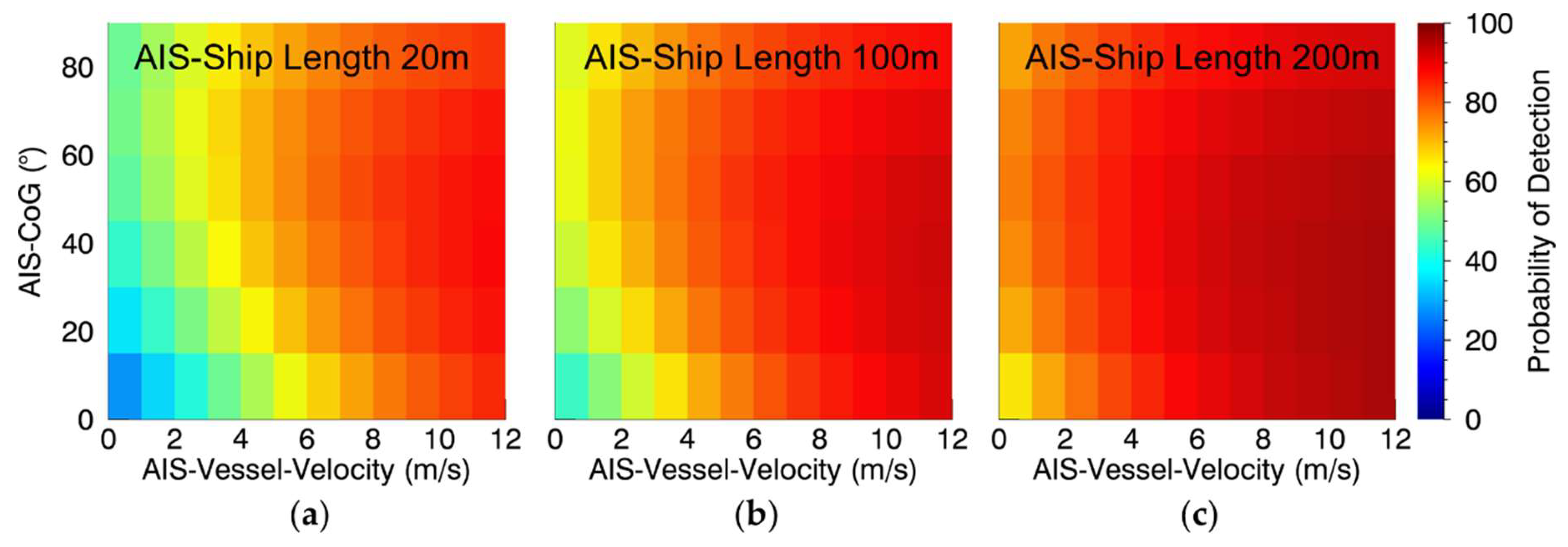
3.4.2. AIS-Vessel-Velocity
3.4.3. AIS-Length
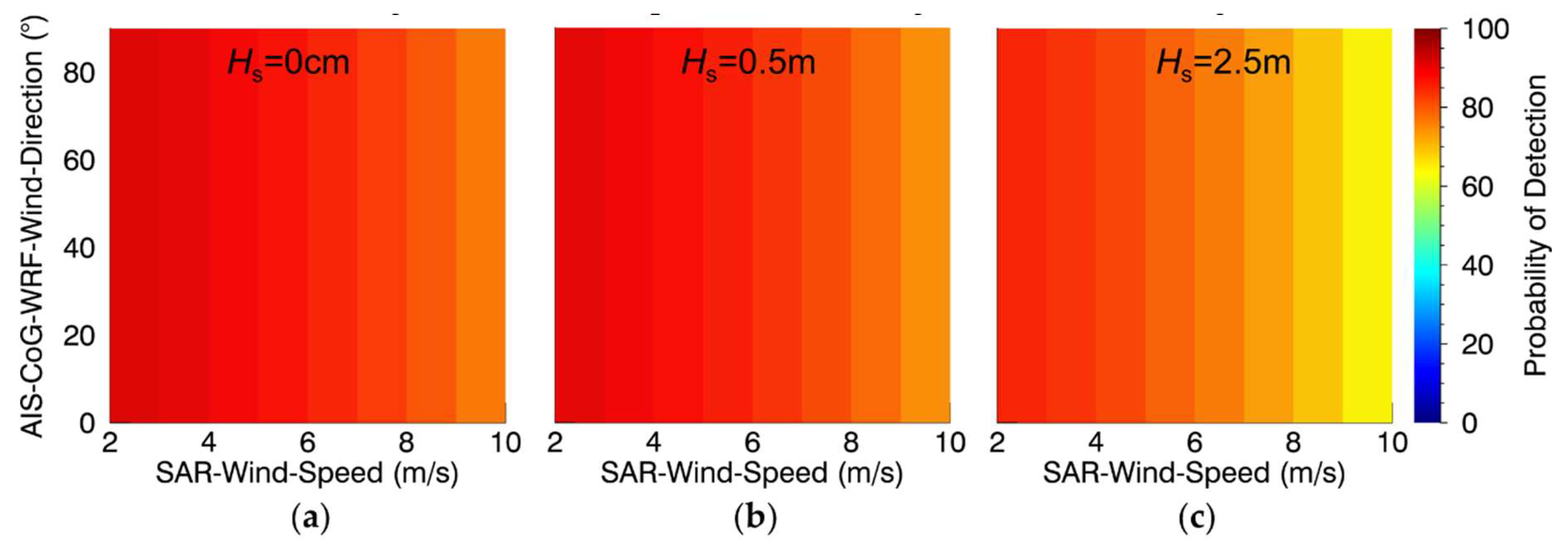
3.4.4. SAR-Wind-Speed
3.4.5. SAR-Significant-Wave-Height
3.4.6. AIS-CoG
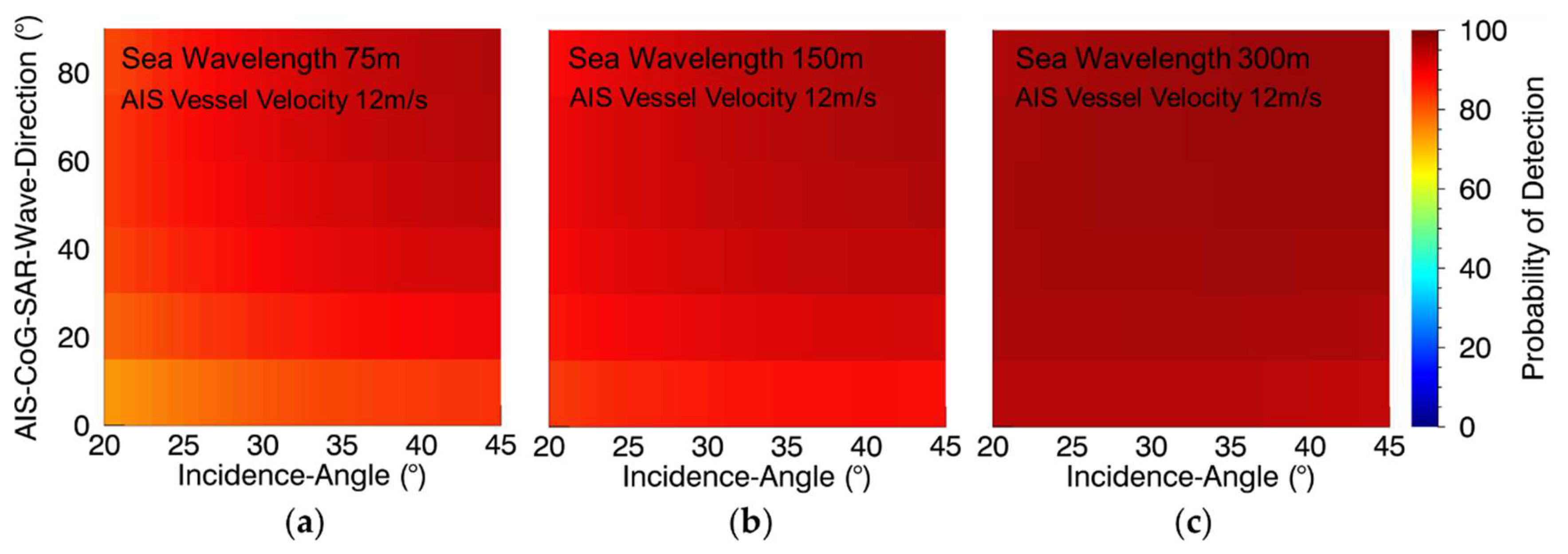
3.4.7. AIS-CoG-SAR-Wave-Direction
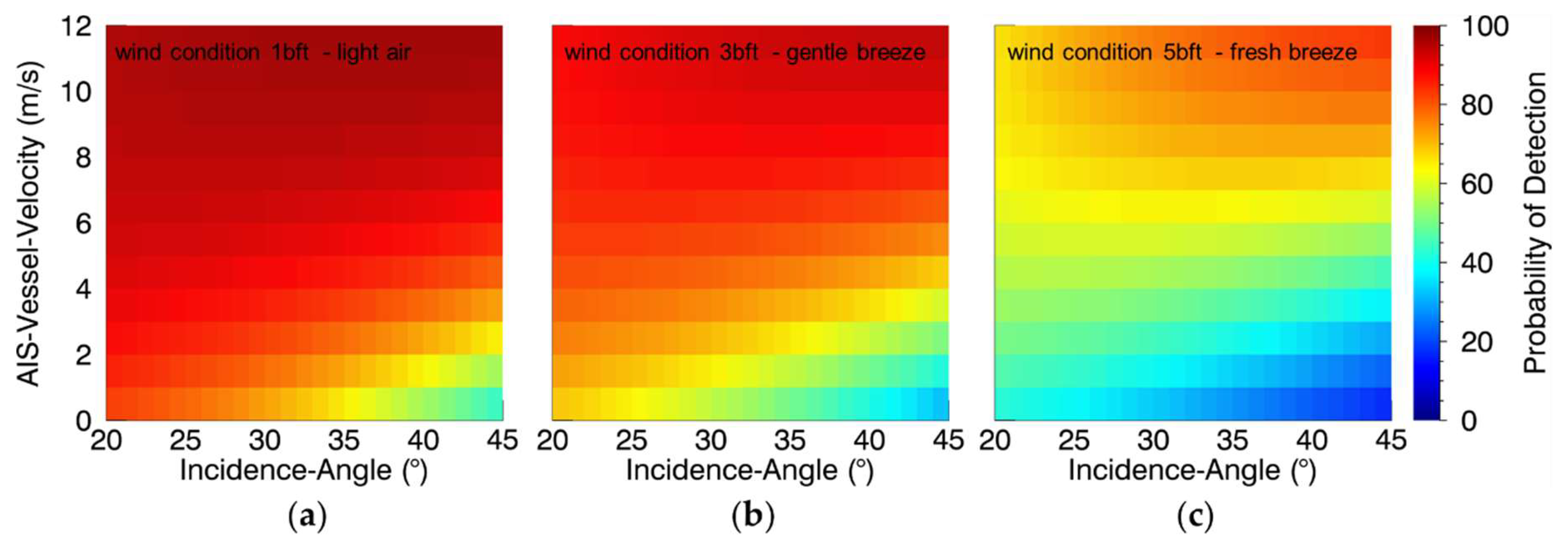
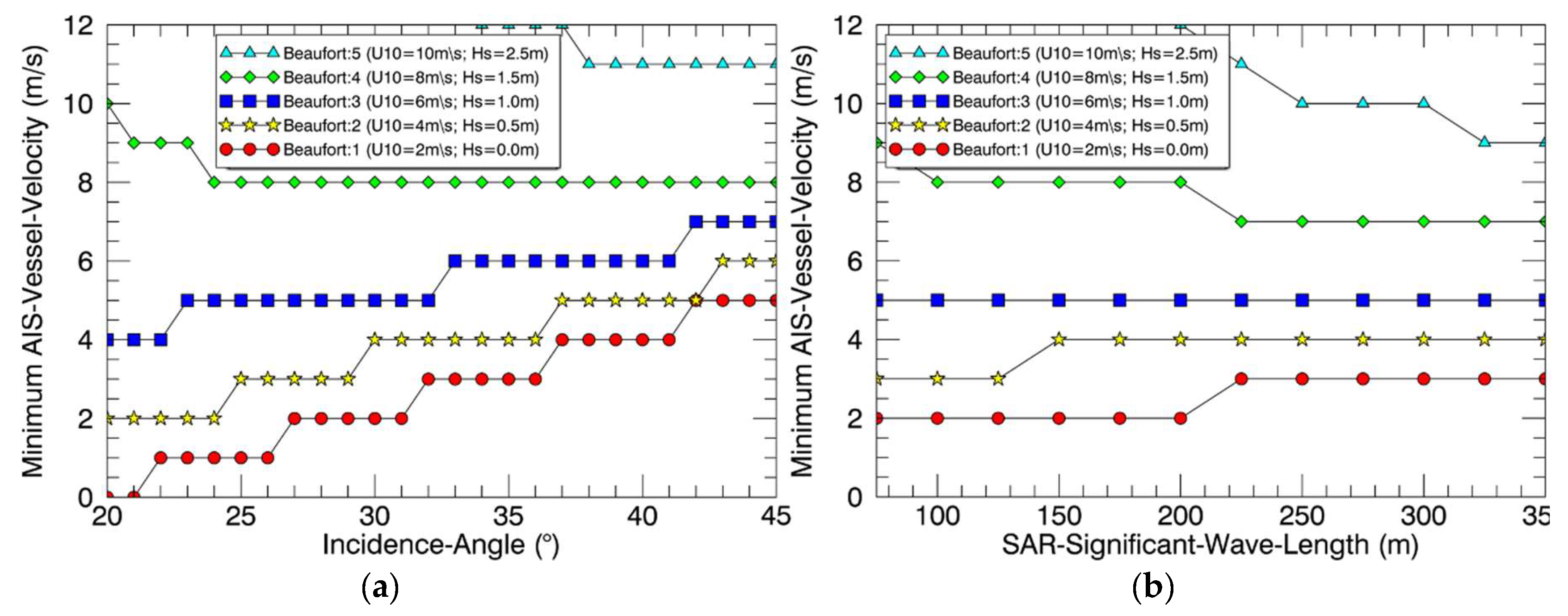
3.4.8. Incidence-Angle
- For smooth ocean surface the turning point is located around 9 m/s of AIS-Vessel-Velocity:
- o
- Below 9 m/s with increasing magnitude of Incidence-Angle, the detectability decreases by few percentage points close to 9 m/s up to ~35 percentage points close to 0 m/s
- o
- Above 9 m/s no influence of Incidence-Angle on the detectability is observed
- For rough ocean surface the turning point is located around 6 m/s of AIS-Vessel-Velocity:
- o
- Below 5 m/s with increasing magnitude of Incidence-Angle, the detectability decreases by few percentage points close to 6 m/s up to ~20 percentage points close to 0 m/s
- o
- Above 5 m/s with increasing magnitude of Incidence-Angle, the detectability increases by few percentage points close to 6 m/s up to ~20 percentage points close to 12 m/s
- This means, the turning point, at which the gradient of detectability’s variation of Incidence-Angle switches its sign, decreases from 9 m/s to 6 m/s when the ocean surface gets rougher.
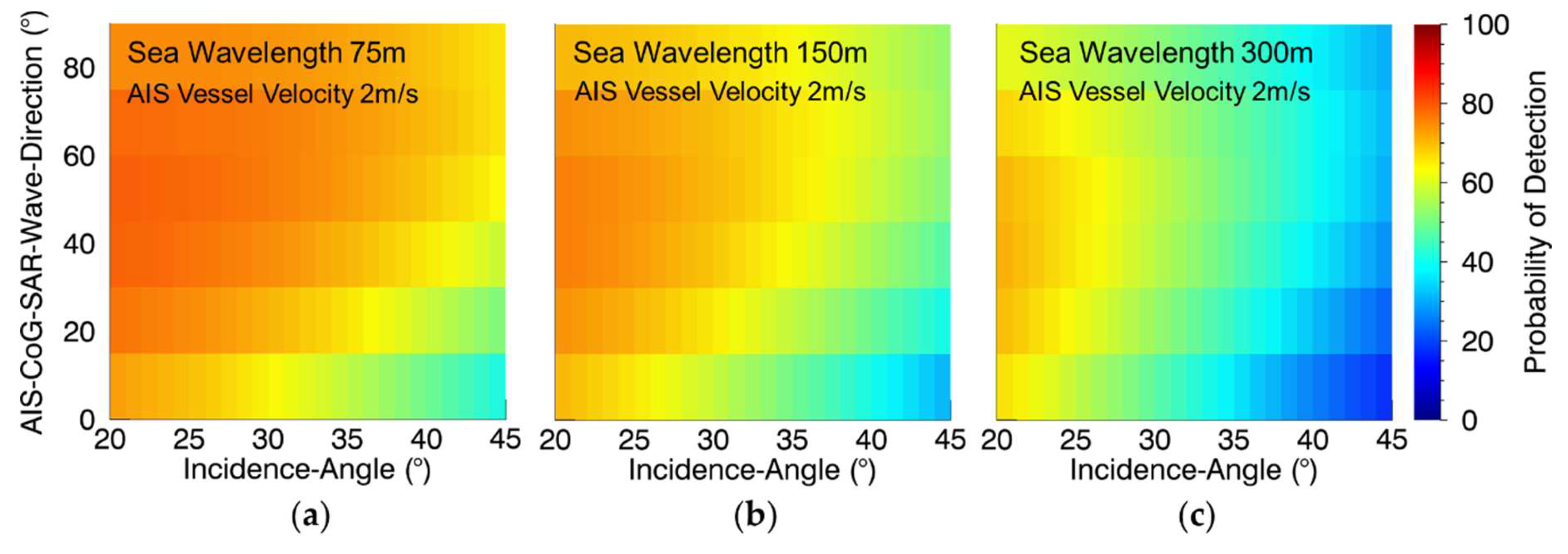
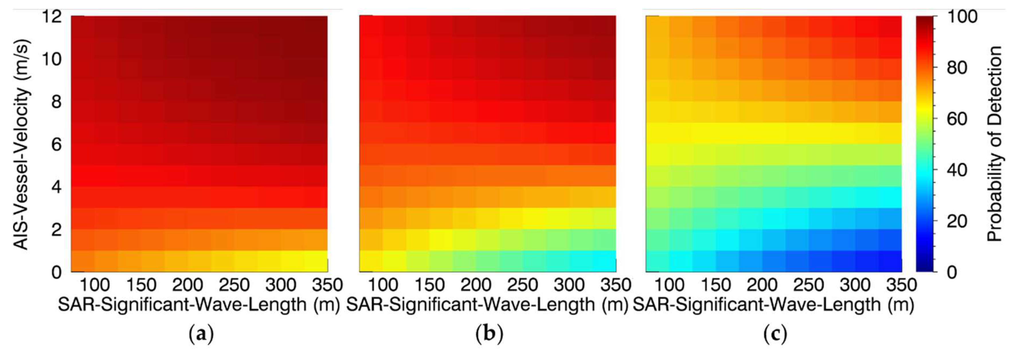
3.4.9. SAR-Significant-Wave-Length
- For smooth ocean surface the turning point is located around 3 m/s of AIS-Vessel-Velocity:
- o
- Below 3 m/s with increasing magnitude of SAR-Significant-Wave-Length, the detectability decreases by few percentage points close to 3 m/s up to ~10 percentage points close to 0 m/s
- o
- Above 3 m/s with increasing magnitude of SAR-Significant-Wave-Length, the detectability increases by few percentage points close to 3 m/s up to ~5 percentage points close to 12 m/s
- For rough ocean surface the turning point is located around 6 m/s of AIS-Vessel-Velocity:
- o
- Below 6 m/s with increasing magnitude of SAR-Significant-Wave-Length, the detectability decreases by ~5 percentage points close to 6 m/s up to ~25 percentage points close to 0 m/s
- o
- Above 6 m/s with increasing magnitude of SAR-Significant-Wave-Length, the detectability increases by few percentage points close to 6 m/s up to ~20 percentage points close to 12 m/s
- This means, the turning point, at which the gradient of detectability’s variation of SAR-Significant-Wave-Length switches its sign, increases from 3 m/s to 6 m/s when the ocean surface gets rougher
4. Discussion
4.1. AIS-CoG-WRF-Wind-Direction
4.2. AIS-Vessel-Velocity
- First, a larger velocity results in a more extensive area of the ocean surface being affected in a shorter time and larger wake signatures are better recognizable.
4.3. AIS-Length
4.4. SAR-Wind-Speed and SAR-Significant-Wave-Height
4.5. AIS-CoG
4.6. AIS-CoG-SAR-Wave-Direction
4.7. Incidence-Angle
4.8. SAR-Significant-Wave-Length
5. Applications
6. Conclusions
- The higher the vessel velocity the higher the detectability
- The radar beam looking direction and the ocean waves’ traveling direction should be perpendicular to the angle of Kelvin wake arms for higher detectability
- Rough, inhomogeneous ocean surface conditions worsen the detectability
- Slow ships are better detectable with lower incidence angles or shorter wavelengths of ocean surface waves and fast ships are better detectable with higher incidence angles and longer wavelengths of ocean surface waves
Author Contributions
Funding
Acknowledgments
Conflicts of Interest
References
- Tings, B.; Bentes, C.; Lehner, S. Dynamically adapted ship parameter estimation using TerraSAR-X images. Int. J. Remote Sens. 2016, 37, 1990–2015. [Google Scholar] [CrossRef]
- Copeland, A.C.; Ravichandran, G.; Trivedi, M.M. Localized Radon Transform-Based Detection of Ship Wakes in SAR Images. IEEE Trans. Geosci. Remote Sens. 1995, 33, 35–45. [Google Scholar] [CrossRef]
- Eldhuset, K. An Automatic Ship and Ship Wake Detection System for Spaceborne SAR Images in Coastal Regions. IEEE Trans. Geosci. Remote Sens. 1996, 34, 1010–1019. [Google Scholar] [CrossRef]
- Crisp, D.J. The State-of-the-Art in Ship Detection in Synthetic Aperture Radar Imagery; DSTO Information Sciences Laboratory: Edinburgh, Scotland, 2004. [Google Scholar]
- Graziano, M.D.; D’Errico, M.; Rufino, G. Wake Component Detection in X-Band SAR Images for Ship Heading and Velocity Estimation. Remote Sens. 2016, 6, 498. [Google Scholar] [CrossRef]
- Biondi, F. Low-Rank Plus Sparse Decomposition and Localized Radon Transform for Ship Wake Detection in Synthetic Aperture Radar Images. IEEE Geosci. Remote Sens. Lett. 2017, 15, 117–121. [Google Scholar] [CrossRef]
- Biondi, F. (L+ S)-RT-CCD for Terrain Paths Monitoring. IEEE Geosci. Remote Sens. Lett. 2018, 15, 1209–1213. [Google Scholar] [CrossRef]
- Biondi, F. A Polarimetric Extension of Low-Rank Plus Sparse Decomposition and Radon Transform for Ship Wake Detection in Synthetic Aperture Radar Images. IEEE Geosci. Remote Sens. Lett. 2018, 16, 75–79. [Google Scholar] [CrossRef]
- Schurmann, S.R. Radar characterization of ship wake signatures and ambient ocean clutter features. IEEE Aerosp. Electron. Syst. Mag. 1989, 4, 182–187. [Google Scholar] [CrossRef]
- Vachon, P.; Campbell, J.; Bjerkelund, C.; Dobson, F.; Rey, M. Ship Detection by the RADARSAT SAR: Validation of Detection Model Predictions. Can. J. Remote Sens. 1997, 23, 48–59. [Google Scholar] [CrossRef]
- Vachon, P.; Wolfe, J.; Greidanus, H. Analysis of Sentinel-1 marine applications potential. In Proceedings of the 2012 IEEE International Geoscience and Remote Sensing Symposium, Munich, Germany, 22–27 July 2012. [Google Scholar]
- Vachon, P.; English, R.; Sandirasegaram, N.; Wolfe, J. Development of an X-Band SAR Ship Detectability Model: Analysis of TerraSAR-X Ocean Imagery; Defence R&D Canada: Ottawa, ON, Canada, 2013. [Google Scholar]
- Tings, B.; Bentes, C.; Velotto, D.; Voinov, S. Modelling Ship Detectability Depending On TerraSAR-X-derived Metocean Parameters. CEAS Space J. 2018, 1–14. [Google Scholar] [CrossRef]
- Tings, B.; Velotto, D. Comparison of ship wake detectability on C-band and X-band SAR. Int. J. Remote Sens. 2018, 39, 4451–4468. [Google Scholar] [CrossRef]
- Hennings, I.; Romeiser, R.; Alpers, W.; Viola, A. Radar imaging of Kelvin arms of ship wakes. Int. J. Remote Sens. 1999, 20, 2519–2543. [Google Scholar] [CrossRef]
- Alpers, W.R.; Ross, D.B.; Rufenach, C.L. On the detectability of ocean surface waves by real and synthetic aperture radar. J. Geophys. Res. 1981, 86, 6481–6498. [Google Scholar] [CrossRef]
- Panico, A.; Graziano, M.D.; Renga, A. SAR-Based Vessel Velocity Estimation From Partially Imaged Kelvin Pattern. IEEE Geosci. Remote Sens. Lett. 2017, 14, 2067–2071. [Google Scholar] [CrossRef]
- Zilman, G.; Zapolski, A.; Marom, M. On Detectability of a Ship’s Kelvin Wake in Simulated SAR Images of Rough Sea Surface. IEEE Trans. Geosci. Remote Sens. 2015, 53, 609–619. [Google Scholar] [CrossRef]
- Lyden, J.D.; Hammond, R.R.; Lyzenga, D.R.; Shuchman, R. Synthetic Aperture Radar Imaging of Surface Ship Wakes. J. Geophys. Res. 1988, 93, 12293–12303. [Google Scholar] [CrossRef]
- Reed, A.M.; Milgram, J.H. Ship Wakes and Their Radar Images. Annu. Rev. Fluid Mech. 2002, 34, 469–502. [Google Scholar] [CrossRef]
- Soloviev, A.; Gilman, M.; Young, K.; Brusch, S.; Lehner, S. Sonar Measurements in Ship Wakes Simultaneous with TerraSAR-X Overpasses. IEEE Trans. Geosci. Remote Sens. 2010, 48, 841–851. [Google Scholar] [CrossRef]
- Milgram, J.H.; Peltzer, R.D.; Griffin, O.M. Supression of Short Sea Waves in Ship Wakes: Measurements and Observations. J. Geophys. Res. 1993, 98, 7103–7144. [Google Scholar] [CrossRef]
- Alpers, W.; Romeiser, R.; Hennings, I. On the radar imaging mechanism of Kelvin arms of ship wakes. In Proceedings of the IEEE International Geoscience and Remote Sensing, Symposium Proceedings, Seattle, WA, USA, 6–10 July 1998. [Google Scholar]
- Tunaley, J.K.E.; Buller, E.H.; Wu, K.H.; Rey, M.T. The Simulation of the SAR Image of a Ship Wake. IEEE Trans. Geosci. Remote Sens. 1991, 29, 149–156. [Google Scholar] [CrossRef]
- Gu, D.; Phillips, O. On narrow V-like ship wakes. J. Fluid Mech. 1994, 275, 301–321. [Google Scholar] [CrossRef]
- Stapleton, N.R. Ship wakes in radar imagery. Int. J. Remote Sens. 1997, 18, 1381–1386. [Google Scholar] [CrossRef]
- Thompson, D.R.; Gasparovic, R.F. Intensity modulation in SAR images of internal waves. Nature 1986, 320, 345–348. [Google Scholar] [CrossRef]
- Alpers, W. Theory of radar imaging of internal waves. Nature 1985, 314, 245–247. [Google Scholar] [CrossRef]
- Li, X.-M.; Lehner, S. Algorithm for Sea Surface Wind Retrieval from TerraSAR-X and TanDEM-X Data. IEEE Trans. Geosci. Remote Sens. 2014, 52, 2928–2939. [Google Scholar] [CrossRef]
- Shemdin, O.H. Synthetic Aperture Radar Imaging of Ship Wakes in the Gulf of Alaska. J. Geophys. Res. 1990, 95, 16319–16338. [Google Scholar] [CrossRef]
- Gade, M.; Alpers, W.; Hühnerfuss, H.; Wismann, V.R.; Lange, P.A. On the Reduction of the Radar Backscatter by Oceanic Surface Films: Scatterometer Measurements and Their Theoretical Interpretation. Remote Sens. Environ. 1998, 66, 52–70. [Google Scholar] [CrossRef]
- Minchew, B.; Jones, C.E.; Holt, B. Polarimetric Analysis of Backscatter from the Deepwater Horizon Oil Spill Using L-Band Synthetic Aperture Radar. IEEE Trans. Geosci. Remote Sens. 2012, 50, 3812–3830. [Google Scholar] [CrossRef]
- Jacobsen, S.; Lehner, S.; Hieronimus, J.; Schneemann, J.; Kühn, M. Joint Offshore Wind Field Monitoring with Spaceborne SAR and Platform-Based Doppler LiDAR Measurements. Int. Arch. Photogramm. Remote Sens. Spat. Inf. Sci. 2015, 959–966. [Google Scholar] [CrossRef]
- Pleskachevsky, A.; Rosenthal, W.; Lehner, S. Meteo-marine parameters for highly variable environment in coastal regions from satellite radar images. ISPRS J. Photogramm. Remote Sens. 2016, 119, 464–484. [Google Scholar] [CrossRef]
- Skamarock, W.C.; Klemp, J.B.; Dudhia, J.; Gill, D.O.; Barker, D.M.; Duda, M.G.; Huang, X.-Y.; Wang, W.; Powers, J.G. A Description of the Advanced Research WRF Version 3; NCAR Technical Notes; National Center for Atmospheric Research: Boulder, CO, USA, 2008. [Google Scholar]
- Berthold, M.; Hand, D.J. Intelligent Data Analysis—An Introduction; Springer: Heidelberg, Germany, 2003. [Google Scholar]
- Platt, J.C. Probabilistic Outputs for Support Vector Machines and Comparisons to Regularized Likelihood Methods. Adv. Large Margin Classif. 2000, 10, 61–74. [Google Scholar]
- Ben-Hur, A.; Weston, J. A User’s Guide to Support Vector Machines. In Data Mining Techniques for the Life Sciences; Humana Press: Totowa, NJ, USA, 2010; pp. 223–239. [Google Scholar]
- Kohavi, R. A study of cross-validation and bootstrap for accuracy estimation and model selection. In Proceedings of the Fourteenth International Joint Conference on Artificial Intelligence, Montreal, QC, Canada, 20–25 August 1995; Volume 2. [Google Scholar]
- Office, M. Beaufort Wind Force Scale. Met Office. 3 March 2016. Available online: https://www.metoffice.gov.uk/guide/weather/marine/beaufort-scale (accessed on 20 January 2019).
- Wackerman, C.; Clemente-Colón, P. Wave Refraction, Breaking and Other Near-Shore Processes. In Synthetic Aperture Radar; NOAA NESDIS Office of Research and Applications: Washington, DC, USA, 2000; pp. 171–189. [Google Scholar]
- Lehner, S.; Pleskachevsky, A.; Velotto, D.; Jacobsen, S. Meteo-Marine Parameters and Their Variability Observed by High Resolution Satellite Radar Images. J. Oceanogr. 2013, 26, 80–91. [Google Scholar] [CrossRef] [Green Version]
- Rabaud, M.; Moisy, F. Ship wakes: Kelvin or Mach angle? Phys. Rev. Lett. 2013, 110, 21. [Google Scholar] [CrossRef] [PubMed]
- Darmon, A.; Benzaquen, M.; Raphaël, E. Kelvin wake pattern at large Froude numbers. J. Fluid Mech. 2014, 738. [Google Scholar] [CrossRef]
- Kelvin, L. On the waves produced by a single impulse in water of any depth. Proc. R. Soc. Lond. Ser. A 1887, 42, 80–83. [Google Scholar]


| Influencing Parameter Name | Description | Value Range (Default Setting) |
|---|---|---|
| AIS-Vessel-Velocity | Velocity of the vessel derived from AIS messages interpolated to the image acquisition time | 0 m/s to 12 m/s (6 m/s) |
| AIS-Length | Length of the corresponding vessel based on AIS information | 10 m to 390 m (100 m) |
| SAR-Wind-Speed | Wind speed estimated from the SAR background around the vessel using the XMOD-2 geophysical model function [29,33] | 2 m/s to 10 m/s (6 m/s) |
| Incidence-Angle | Incidence angle of the radar cropped to TerraSAR-X’s full performance value range | 20° to 45° (30°) |
| SAR-Significant-Wave-Height | Significant wave height estimated from the SAR background around the vessel using the XWAVE_C empirical model function [34] | 0 m to 3 m (0.5 m) |
| SAR-Significant-Wave-Length | Wave length estimated from the SAR background around the vessel using the XWAVE_C empirical model function [34] | 75 m to 350 m (150 m) |
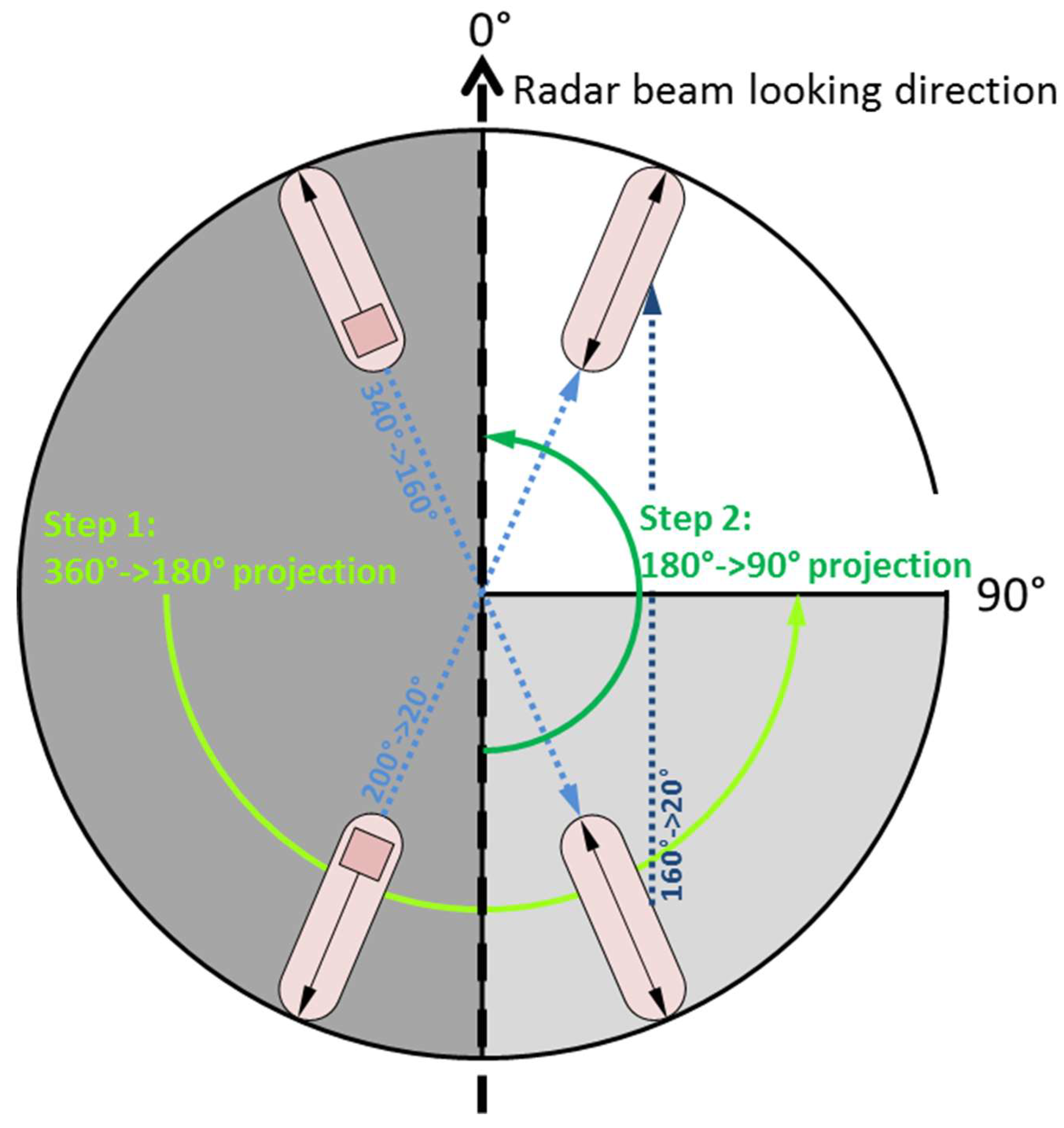
| AIS-CoG-SAR-Wave-Direction | Absolute angular difference between AIS-CoG and wave direction estimated from the SAR background around the vessel using the XWAVE_C empirical model function [34]. The 0°–360° value range has been projected to 0°–90° as displayed in Figure 3. | 0° to 90° (45°) |
| AIS-CoG | The course over ground based on AIS information relative to the radar looking direction (0° means parallel to range and 90° mean parallel to Azimuth). The 0°–360° value range has been projected to 0°–90° as displayed in Figure 3. | 0° to 90° (45°) |
| AIS-CoG-WRF-Wind-Direction | Absolute angular difference between AIS-CoG and wind direction estimated by the Weather Research and Forecasting Model (WRF) [35] nearby the vessel. The 0°–360° value range has been projected to 0°–90° as displayed in Figure 3. | 0° to 90° (45°) |
| Hyperparameter Name | Value |
|---|---|
| Kernel type | polynomial |
| Kernel degree | 2 |
| Cost | 0.1 |
| Gamma | 0.01 |
| Coef0 | 100 |
© 2019 by the authors. Licensee MDPI, Basel, Switzerland. This article is an open access article distributed under the terms and conditions of the Creative Commons Attribution (CC BY) license (http://creativecommons.org/licenses/by/4.0/).
Share and Cite
Tings, B.; Pleskachevsky, A.; Velotto, D.; Jacobsen, S. Extension of Ship Wake Detectability Model for Non-Linear Influences of Parameters Using Satellite Based X-Band Synthetic Aperture Radar. Remote Sens. 2019, 11, 563. https://doi.org/10.3390/rs11050563
Tings B, Pleskachevsky A, Velotto D, Jacobsen S. Extension of Ship Wake Detectability Model for Non-Linear Influences of Parameters Using Satellite Based X-Band Synthetic Aperture Radar. Remote Sensing. 2019; 11(5):563. https://doi.org/10.3390/rs11050563
Chicago/Turabian StyleTings, Björn, Andrey Pleskachevsky, Domenico Velotto, and Sven Jacobsen. 2019. "Extension of Ship Wake Detectability Model for Non-Linear Influences of Parameters Using Satellite Based X-Band Synthetic Aperture Radar" Remote Sensing 11, no. 5: 563. https://doi.org/10.3390/rs11050563