A Comparison of Three Sediment Acoustic Models Using Bayesian Inversion and Model Selection Techniques


1
School of Marine Science and Technology, Tianjin University, Tianjin 300072, China
2
National Ocean Technology Center, Tianjin 300112, China
3
Institute of Geospatial Information, Information Engineering University, Zhengzhou 450052, China
*
Author to whom correspondence should be addressed.
Remote Sens. 2019, 11(5), 562; https://doi.org/10.3390/rs11050562
Submission received: 15 January 2019
/
Revised: 21 February 2019
/
Accepted: 2 March 2019
/
Published: 7 March 2019
(This article belongs to the Special Issue Advances in Undersea Remote Sensing)
Abstract
:Many geoacoustic models are used to establish the relationship between the physical and acoustic properties of sediments. In this work, Bayesian inversion and model selection techniques are applied to compare combinations of three geoacoustic models and corresponding scattering models—the fluid model with the effective density fluid model (EDFM), the grain-shearing elastic model with the viscosity grain-shearing (VGS(λ)) model, and the poroelastic model with the corrected and reparametrized extended Biot–Stoll (CREB) model. First, the resolution and correlation of parameters for the three models are compared based on estimates of the posterior probability distributions (PPDs), which are obtained by Bayesian inversion using the backscattering strength data. Then, model comparison and selection techniques are utilized to assess the matching degree of model predictions and measurements qualitatively and to ascertain the Bayes factors in favor of each quantitatively. These studies indicate that the fluid and poroelastic models outperform the grain-shearing elastic model, in terms of both parameter resolution and the ability to produce predictions in agreement with measurements for sandy sediments. The poroelastic model is considered to be the best, as the inversion based on it can provide more highly resolved information of sandy sediments. Finally, the attempt to implement geoacoustic inversion with different models provides a relatively feasible remote sensing scheme for various types of sediments under unknown conditions, which needs further validation.
1. Introduction
As the main means of underwater investigation, acoustic remote sensing techniques have been a research hotspot over the last decades. Underwater topographic acoustic telemetry has been a great success, leading to the emergence of many highly efficient commercial products, ranging from high-frequency single- and multibeam echosounders and sidescan sonars to low-frequency sub-bottom profiling tools and seismic systems. In the course of investigation using such equipment, sediment sampling has often been done to form a dataset corresponding to the acoustic data, and the sediment samples are used for the verification of seabed classification [1]. Restricted by the time and cost required for collection and analysis of samples, the verification behavior cannot be expanded on a large scale. Indeed, seabed classification just tells us that the sediments are different at different locations. In order to obtain geoacoustic properties of sediments, model-based inversion of acoustic data is a more effective and feasible means compared with grab samples [2].
According to the sediment geoacoustic model categories proposed by Jackson and Richardson [3], there are three categories, which are fluid, elastic, and poroelastic, based on the number and types of acoustic waves that can travel in sediments. We can see from the literature [4,5,6,7,8,9] that these geoacoustic models are mainly used to establish the relationship between physical and acoustic properties of sediments, such as sound speed and attenuation, and are regarded as “wave theory” or “propagation theory” to distinguish them from subsequent scattering models by Jackson and Richardson. In acoustic remote sensing, scattering models of water–seabed interface are necessary to calculate observations such as scattering strength in model-based inversion, since the speed and attenuation of sound in sediments cannot be directly measured from a distance. Similarly, scattering models are also classified into three categories.
Due to the prevalence of sandy sediment in coastal environments, there have been a relatively large number of experimental data/model comparisons corresponding to sandy sediment [10,11,12,13]. The development of models is driven by the mismatch of model prediction and acoustic observation, including sound speed and attenuation, within sediments measured in situ and scattering strength measured remotely. The poroelastic model may be a reasonable choice for a porous medium such as sandy sediment. Biot first proposed a theory of sound propagation in a poroelastic medium, taking into account the interactions between the pore fluid and consolidated elastic frame [14,15]. The theory was first used to model sandy sediments by Stoll [16]. The Biot–Stoll model is a fundamental improvement over the fluid and viscoelastic models and provides a satisfactory fitting performance of model prediction with the measured data [10,13]. Based on the mismatch between model prediction and measured data, Chotiros further extended the Biot–Stoll model to include the physics of grain–grain contact, multiple scattering losses, a more efficient set of input parameters, and a heuristic correction that allows the model to span a wide range of sediment types [17], which was redefined as the corrected and reparametrized extended Biot–Stoll (CREB) model by Bonomo and Isakson [18].
In addition to direct modification of the Biot–Stoll model, Williams presented an acoustic propagation model that approximates a porous medium as a fluid with a bulk modulus and effective density derived from Biot–Stoll theory [19]. It was shown that the dispersion, transmission, reflection, and scattering predicted with this approximate model, which is named the effective density fluid model (EDFM), are very close to the predictions of the full Biot–Stoll theory for sandy sediment [10,12,20]. The approximate effectiveness and limits of EDFM were analyzed by Bonomo and co-workers using the finite element method (FEM) [21]. In order to further improve the matching degree between the measurements and the model predictions [20], two additional physical mechanisms, transfer of heat between the liquid and solid and the effect of granularity, were added to the EDFM [7].
Although the poroelastic model and its approximation are successful to some extent, another kind of geoacoustic model has received considerable attention. Based on the assumption that the shear rigidity modulus of the medium is zero and implying the absence of a skeletal elastic frame, Buckingham proposed the grain-shearing (GS) elastic model [22]. The model was extended to include the effects of viscosity of the molecularly thin layer of pore fluid separating contiguous grains [6]. The extended version is named VGS, with the first initial serving as a reminder that the model includes viscosity of the pore fluid. The latest version of Buckingham’s model is designated the VGS(λ), with a modification to ensure that the viscosity of the pore fluid has no effect on the shear wave. The shear dispersion relations in the VGS and GS theories are identical. At the same time, Buckingham showed the adequate matching performance of the model prediction with the measured data [8,23].
The main content of the current paper is to compare the performance of inversions based on the three models, EDFM, VGS(λ), and CREB, and their corresponding acoustic scattering models. Bayesian model selection techniques are used to evaluate the degree of matching between model predictions and measurements, which are backscattering strengths in this paper. In fact, this is not the first time that Bayesian techniques have been applied to underwater acoustics. Dosso and co-workers successfully applied Bayesian techniques to estimate the number of seabed layers and the uncertainty of seabed parameters [24,25,26]. There have also been attempts to use Bayesian techniques to solve the problem of seabed sediment classification [27,28]. Bayesian inversion and model selection based on the geoacoustic models using sound speed and attenuation measurements were carried out by Bonomo and Isakson to compare the competing geoacoustic models [18]. In this work, we introduce a similar comparison for underwater remote sensing by combining the geoacoustic models with corresponding scattering models, using scattering strength measurements to carry out inversion and model selection. The authors believe this is the first time that model selection techniques have been applied to underwater remote sensing using scattering strength to compare different types of models. Before parameter inversion, a parameter sensitivity analysis is carried out to forecast the relative resolution of parameters of each model and provide an interpretation of the subsequent inversion results. Then, the resolution of parameters that are mostly difficult to measure in situ can be obtained from inversion results and compared with the results of the sensitivity analysis. The model selection techniques can provide a quantitative measure of the most suitable model. When faced with a complex and unknown sediment environment, the comparison can also provide a relatively feasible scheme for assessing different kinds of models for underwater acoustic inversion and remote sensing, and the best model and inversion results for specific sediment can be obtained.
The observation used in the inversion is backscattering strength varying with angle and frequency. Since this paper is mainly concerned with the uppermost layer of sediment and the scattering model used here is only suitable for high frequency, the backscattering strength measurements are carried out at high frequencies (≥100 kHz). The remainder of this paper has the following organization. The calculation processes of scattering strength for the three models and corresponding model parameter sensitivity analysis are given in Section 2. Section 3 briefly reviews the Bayesian inference method used in this work. Section 4 presents the experimental measurements, parameter inversion, and model selection results. Finally, this work is concluded in Section 5.
2. Geoacoustic Models and Acoustic Scattering Models
Geoacoustic models are usually established to describe the relationship between physical parameters and the attenuation and speed of sound waves that propagate within sediment, as mentioned above. The main content of this section is a combination of the latest geoacoustic and scattering models used to calculate scattering strength. According to the model categories proposed by Jackson and Richardson [3], a fluid medium only supports the propagation of compressional waves, an elastic medium supports the propagation of compressional waves and shear waves, and a poroelastic medium supports additional slow compressional waves compared to the elastic medium. It is important to note that slow compressional waves are given theoretically and have never been observed in natural marine sediment. The combination means that the attenuation and speed of sound waves supported by the corresponding geoacoustic model categories are needed as input for different kinds of scattering models. Indeed, different kinds of geoacoustic and scattering models can be applied in cross-combinations to calculate scattering strength. The EFDM is an example in which effective density derived from the Biot–Stoll theory is used to calculate scattering strength based on fluid scattering models. Then the fluid scattering model is extended to the poroelastic case by the simple replacement of density by effective density.
Although the separation of scattering into separate, independent roughness and volume components is somewhat artificial, it is helpful to understand the scattering mechanisms by discussing them separately. The total scattering strength can be expressed as
where and denote scattering cross-sections of rough water–seabed interface and volume heterogeneities, respectively. As mentioned above, due to the prevalence of sandy sediment, the study in this paper is also based on sandy sediment. At high frequencies, the scattering of sandy sediment is mainly due to interface roughness scattering [10], which is modeled by three types of models, and the contribution from a fluid volume scattering model is included for completeness in this paper. Through the cross-combination mentioned above, the fluid volume scattering model can also be extended to the elastic and poroelastic case. The following are the calculation processes of scattering strength of the fluid model, grain-shearing elastic model, and poroelastic model, and the corresponding model parameter sensitivity analysis.
2.1. Fluid Model
Although seabed sediments are composed of discrete particles, it is a reasonable approximation that they are regarded as a continuous medium [29] and this assumption applies to all models used in this paper. As a relatively simple approach, fluid theories are commonly used to describe sediment acoustic properties and have been combined with scattering models. The EFDM, which is proposed as a fluid approximation of the Biot–Stoll theory, extends the fluid model input parameters to the poroelastic case. The calculation process of this approximation only considers the propagation of compressional waves in sediments, leading to its category as a fluid type. The fluid model used here to calculate the scattering strength requires 15 input parameters—roughness spectral exponent , roughness spectral strength , density fluctuation spectral exponent , density fluctuation spectral strength , ratio of compressibility to density fluctuation in sediment , mean grain diameter , tortuosity , porosity , dynamic viscosity of water , permeability , mass density of water , mass density of grains , bulk modulus of water , bulk modulus of grains , and compressional wave speed in water .
2.1.1. EDFM
The fluid model used in this paper has been extended to the poroelastic case by using the effective density. Therefore, the calculation of scattering strength needs to begin from the relevant parameters of the poroelastic theory. Based on the Biot constitutive relations, four moduli are given successively by Stoll, and the relationships between the moduli and the parameters of constituent media are as follows [30]:
where is the complex frame bulk modulus and is the complex frame shear moduli. The starting point of the EDFM regarded as an approximation for full Biot–Stoll is the frame modulus set to zero. The reason for this is that the frame moduli are small and can be negligible compared with the grain and water moduli. Then an effective fluid modulus can be obtained:
The effective fluid modulus is substituted into the wave equation of the Biot theory, and the detailed derivation process can be found in [19]. The effective density, complex acoustic compressional speed, and corresponding phase speed in sediment can be obtained by:
where , is the acoustic frequency, and is the complex correction factor for dynamic viscosity:
where and are Bessel functions of the first kind, and is called the pore size. In order to further improve the matching degree between model predictions and measurements of sound speed and attenuation, Williams added two additional nongrain contact mechanisms to the EDFM: heat transfer between the liquid and solid at low frequencies and granularity of the medium at high frequencies [7]. Since the application of the EDFM in this paper is at high frequencies, only the model modification using doublet mechanics (DM) to model the granularity for high frequency is given here. This is done by adding a correction factor to as follows:
where is the wavelength of sound wave in water and can be obtained by:
where are direction cosines and functions of , and the expressions are: , , . The additional multiple scattering loss is added into the attenuation () by [31]:
The final modified complex compressional wave speed can be expressed as:
The complex speed ratio and density ratio needed to calculate the scattering strength in the scattering model are:
2.1.2. Fluid Interface Roughness Scattering Model
For roughness scattering at the sea bottom interface, two widely used approximations are used to calculate the scattering strength: the small-roughness perturbation method and the Kirchhoff approximation. The perturbation theory tends to be most accurate for scattering at wide angles relative to the specular (flat-interface reflection) direction [32], and the Kirchhoff approximation is better for scattering near the specular direction [33]. The approximation method used in this paper is called small-slope approximation; it was first proposed by Voronovich to study scattering by the sea surface [34] and was subsequently used to study seabed scattering. In the interest of simplicity, the lowest-order small-slope approximation is used, which can provide a single expression that covers all angles and is likely to be at least as accurate as either the Kirchhoff or perturbation approximation. According to the summary by Jackson, the uniform expression of roughness scattering cross-section for different models using lowest-order small-slope approximation is [3]:
where is the acoustic wavenumber in water and , denote the magnitude of the horizontal and vertical vector difference between the scattered wave and the incident wave, respectively, and are given in Appendix A.
Assuming that the roughness is isotropic and follows pure power law, can be obtained by:
where is the square of the “structure constant,” which is related to the parameters of the power-law spectrum through:
where is the gamma function. The above calculation process of roughness scattering cross-section is also applicable to the grain-shearing elastic and poroelastic models. The difference is the calculation of . The expression of factor for the fluid model is:
where , , and are defined in Figure A1. is the flat-interface reflection coefficient and can be obtained by:
2.1.3. Fluid Volume Scattering Model
Although the acoustic scattering caused by the inhomogeneity of sediments is more significant only in soft seabeds, such as muddy seabed, where sound waves can easily travel in and out, the volume scattering is taken as a supplement and modification for total scattering strength to further enhance the matching performance of the models. The small-perturbation fluid approximation for volume scattering is used. Assuming that the volume scattering strength is independent of depth, the expression for is [35,36]:
where is the real part of the vector difference of the scattered and incident waves that propagate in sediment, given in Appendix A. So far, the scattering strength for the fluid model can be obtained through Equations (1), (18), and (26).
2.2. Grain-Shearing Elastic Model
The categories of models discussed by Jackson and Richardson are meant to be broad and can apply to consolidated sediments such as rock where model proposed by Buckingham is designed for unconsolidated sediments such as sand. In order to distinguish the elastic model used in this paper from the empirical visco-elastic model developed by Hamilton [37], the term ‘grain-shearing elastic model’ is used to specify the combination of VGS(λ) and elastic scattering model. Compared with the fluid model, the grain-shearing elastic model incorporates shear forces. The sediment supports the propagation of shear waves, which is modeled to provide additional corrections. The grain-shearing elastic model used here to calculate the scattering strength requires 16 input parameters: roughness spectral exponent , roughness spectral strength , density fluctuation spectral exponent , density fluctuation spectral strength , ratio of compressibility to density fluctuation in sediment , porosity , mass density of water , mass density of grains , bulk modulus of water , bulk modulus of grains , material exponent , compressional rigidity coefficient , shear rigidity coefficient , compressional viscoelastic relaxation time , shear viscoelastic relaxation time , and compressional wave speed in water .
2.2.1. VGS(λ)
As the latest version of the model proposed by Buckingham, VGS(λ) is an extension of GS that includes the effects of viscosity of the molecularly thin layer of pore fluid separating contiguous grains and a slight modification of the shear viscoelastic relaxation time. The VGS(λ) dispersion curves have also been verified by the measurements in SAX99 [8].
First, Wood’s equation, which usually gives a rather poor prediction of sediment sound speed [38], is given, as it ignores much of the dynamics of the grain-pore water system:
From the view of expression, the VGS() expressions can be considered as modifications of and the compressional wave speed , attenuation , shear wave speed , and attenuation , respectively, are expressed as [6]:
where is the shear viscoelastic relaxation time and is taken because of the experimental evidence [8] that . Then the complex compressional wave speed and shear wave speed can be similarly obtained by Equation (15). The complex speed ratio and can be obtained by Equation (16). The density ratio for the grain-shearing elastic model is as follows:
2.2.2. Elastic Scattering Model
The expression of scattering cross-section for the elastic interface roughness scattering model is similar to the one used with the fluid model. The difference is the factor used in Equation (18), which can be obtained by [3]:
where , given in Appendix B; is the flat-interface reflection coefficient, which can be obtained by Equation (24); and the corresponding for the elastic scattering model is:
As mentioned above, the fluid volume model can be extended for use in an elastic medium by substituting the appropriate parameters into Equations (26) and (27). Then the total scattering strength for the grain-shearing elastic model can be obtained by Equation (1).
2.3. Poroelastic Model
Both elasticity and porosity of sediments are considered in the poroelastic model, where the sediment grains constitute an elastic “frame” coupled to the pore fluid. This is the reason that the poroelastic model supports additional “slow” compressional waves compared with the elastic model. This model is essentially the most appropriate for sandy sediment, which is composed of grains and water as a two-phase system [16]. The total poroelastic model requires 19 input parameters: roughness spectral exponent , roughness spectral strength , density fluctuation spectral exponent , density fluctuation spectral strength , ratio of compressibility to density fluctuation in sediment , mean grain diameter , porosity , dynamic viscosity of water , mass density of water , mass density of grains , bulk modulus of water , bulk modulus of grains , cementation exponent , pore shape factor , Poisson’s ratio of grains , low-frequency asymptotic frame bulk modulus , high-frequency asymptotic increase , bulk relaxation frequency , and compressional wave speed in water .
2.3.1. CREB
In order to reproduce the frequency dependence of the measured sound speed and attenuation and achieve a better matching degree between model predictions and measurements, grain contact physics models have been developed and tested for the poroelastic model. Chotiros and Isakson used grain contact squirt flow and viscous drag mechanisms to better model the observed behavior of attenuation [4]. Then a missing relaxation mechanism was added at higher frequencies related to the grain contact physics, and the extended Biot model was proposed to achieve further improvement [9]. The model used here is the latest version in which the extended Biot model is reparametrized and corrected to be able to model sediments of multiple types [17].
Permeability and tortuosity can be related to the CREB parameters through:
Based on the extended Biot model, the complex effective frame bulk modulus and frame shear modulus are replaced by frequency-dependent expressions:
where can be set equal to 1 for sandy sediment or to other values to model different types of sediments. The moduli , , , complex correction factor can be obtained by Equations (2)–(4) and (10) and the “fast” and “slow” compressional wavenumbers can be expressed as the roots of the following expression:
where root with a negative imaginary component and a smaller real component is the “fast” compressional wavenumber, and root is the “slow” compressional wavenumber. The shear wavenumber is the root with a negative imaginary component of the following expression:
The density ratio for the poroelastic model is the same as that of the grain-shearing elastic model, and the speed ratio can be obtained by:
2.3.2. Poroelastic Scattering Model
Similar to the elastic scattering model, the scattering cross-section for the poroelastic interface roughness scattering model can be obtained by Equation (18), and the corresponding factor is the first element of the following column matrix [39]:
which can be computed by:
where the subscripts of are used to distinguish the two matrices without specific meaning and the superscripts of matrices , , and correspond to the three spatial components. The matrices , , , and are given in Appendix B. is a six-row column vector comprising five reflection and transmission coefficients and supplemented with unity in the last row. The flat-interface reflection coefficient for the poroelastic model is the first element of the column vector . Then the volume scattering can also be computed by Equations (26) and (27) and the total scattering strength for the poroelastic model can be obtained by Equation (1).
2.4. Sensitivity Analysis
Parameter sensitivity analysis is from the view of mathematics and is a global analysis method. The potential correlation between some parameters is not specified in advance and is not considered in the analysis process. Since model predictions of some parameter combinations may not be consistent with local measurements, the parameter resolution given by the results of the sensitivity analysis may not be exactly consistent with that given by inversion results. However, we can still obtain a preliminary understanding of the resolutions of the model parameters through sensitivity analysis. The sensitivity analysis can forecast the relative resolution of parameters for each model and provides an interpretation of the subsequent inversion results. Similar to many global sensitivity analysis methods, the uncertainty importance measure proposed by Borgonovo is used here [40]. Borgonovo verified that the parameter that influences variance the most is not necessarily the parameter that influences the output distribution the most, and proved the effectiveness of his method over other variance-based methods [41,42,43,44]. The definition of the first-order Borgonovo index is:
where is the probability distribution of the model prediction and is the conditional distribution on . indeed is a measure of the expected shift in the probability distribution of the model prediction when is set to a fixed value.
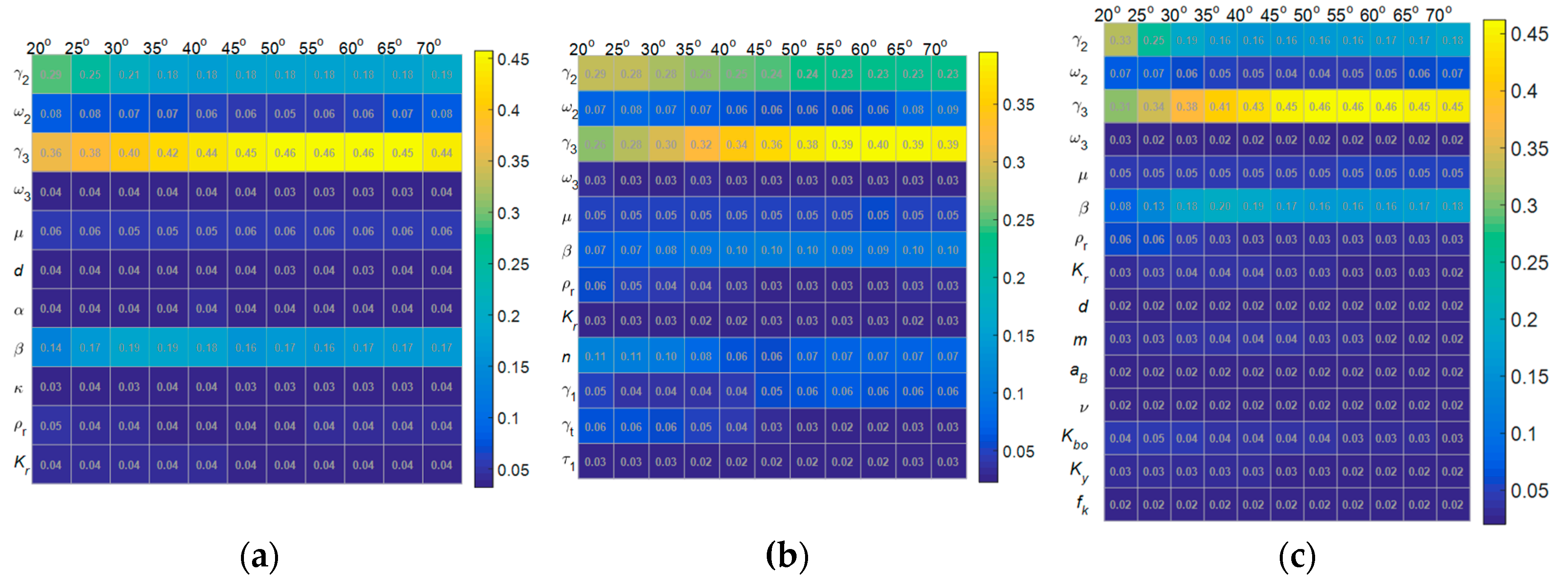
The parameter space is determined for sandy sediments based on the results from previous research in the literature. Bounded, uniform distributions are taken as the parameter priors, and the distribution parameters are given in Table 1, where they are divided into the common parameters of the three models and the unique parameters of each model. The priors are chosen to be minimally informative and represent attempts at capturing the full range of possible values the model input parameters can take for sandy sediments. As shown in Table 2, the parameters that describe the characteristics of water and the sound speed in water are supposed to be known parameters, which refer to water parameters listed in [45]. The reason is that the subsequent experiments are carried out in a rectangular tank filled with fresh water. It should be noted that the mass density and bulk modulus of grains are replaced by ratios to water for convenience, as shown in Table 1. The sensitivity analysis here and the subsequent parameter inversions are both based on these priors. Using Latin hypercube sampling [46], 60,000 samples are generated to calculate the Borgonovo index for each model. The grazing angle range and frequency, respectively, are 20°–70° and .
Figure 1a displays the Borgonovo indices for the fluid model. Inspection of the figure reveals that the roughness spectral exponent , density fluctuation spectral exponent , and porosity have a great influence on model prediction. The effect on the model prediction of roughness spectral strength and ratio of compressibility to density fluctuations is smaller than that of the first three parameters but larger than that of all the remaining parameters. This means that there could be five parameters that yield better resolution in the fluid model-based inversion. Figure 1b shows that the roughness spectral exponent and density fluctuation spectral exponent still have a significant impact on model prediction for the grain-shearing elastic model, while roughness spectral strength , ratio of compressibility to density fluctuation , porosity , and material exponent only have a moderate effect on model prediction. For the poroelastic model in Figure 1c, the sensitive parameters are roughly the same as the fluid model, and the others remain insensitive to model prediction. From Figure 1, we can also see that the indices of some parameters fluctuate under different grazing angles. Indeed, sensitivity analysis was also performed at different frequencies, and the results show that the frequency change had only a slight effect on the indices. Thus, we only give results of sensitivity analysis at here.
3. Bayesian Inference
Bayesian inference is by far the most suitable solution to the inversion problem, as it treats all the parameters as random variables. The inversion results are given in the form of posterior probability distribution (PPD) with quantized uncertainty instead of point estimation based on the global optimization algorithm. This section only makes a brief review; more complete treatments of Bayesian inference applied to geoacoustic inversion can be found elsewhere [24,25,47,48,49]. When a set of observations (scattering strength) and the adopted model for inversion are determined, the PPD of parameter vector can be expressed as
where is the prior probability distribution of . is the conditional probability distribution of observations given model parameters and model . is independent of and is usually considered as a constant factor. Then the PPD can be written as
where is also known as the likelihood function . In order to define the likelihood function, the error of observations, which consists of measurement error and model error, needs to be specified. An effective approach is used here in which the errors of observations are taken as unknown random parameters, like input parameters for model prediction, and estimated simultaneously within the inversion process. Assuming common independent Gaussian-distributed errors, the likelihood function can be expressed as
where is the dimension of ; is the standard deviation for , which is the ith element of ; and is the ith element of , which denotes the observations predicted by the parameter vector and corresponding model . The solution of the inversion problem is given in the form of a marginal PPD, defined as:
where and represent the elements of parameter vector and and denote the one- and two-dimensional marginal PPD, respectively. The integral that needs to be solved can be rewritten as:
For nonlinear problems, such as geoacoustic inversion, the integral does not have an analytic solution. Based on Monte Carlo theory, we can rewrite the integral as:
If a large number of samples , … is obtained from , the integral can be approximately equal to:
Let , then the integral can be further simplified to:
which means that the main objective of inversion is to obtain a set of samples from the PPD to approximate the target integral. It is not difficult to figure out that a larger number of samples that follow the target probability distribution can better approximate the true value of the integral. The rigorous sampling methods will be given in the next section.
3.1. Parameter Inversion
Monte Carlo theory provides the idea that samples can be used to approximate an integral without an analytic expression. Then the key task of parameter inversion is to generate a set of samples that can fully represent the target probability distribution. Compared with the static simulation of traditional Monte Carlo integral, the Markov chain Monte Carlo (MCMC) method is a dynamic simulation as the process goes on. MCMC exploits a Markov chain that generates a random walk through the parameter search space to obtain solutions with stable frequencies stemming from a stationary distribution. Different MCMC methods have different constructions of transfer probability, which has a crucial influence on the convergence efficiency of the Markov chain. The earliest MCMC approach is the random walk Metropolis. Considering nonsymmetrical jumping distributions, Hastings extended the random walk Metropolis algorithm to more general cases, which is known as the Metropolis–Hastings (M–H) algorithm [50]. In order to increase the sampling efficiency of complex posterior distributions involving long tails, correlated parameters, multimodality, and numerous local optima, more improved algorithms have been proposed, such as adaptive proposal (AP) [51], adaptive Metropolis (AM) [52], delayed rejection adaptive Metropolis (DRAM) [53], differential evolution Markov chain (DE-MC) [54], fast Gibbs sampling (FGS) [47], and so on. The sampling method used in this paper is a relatively efficient multichain method called differential evolution adaptive Metropolis (DREAM), which can maintain detailed balance and ergodicity with excellent performance on a wide range of problems involving nonlinearity, high dimensionality, and multimodality [55]. In general, the probability of accepting candidate state as the next state of within the Markov chain is:
where and are the posterior probability densities of parameter vectors at different times, and and are the conditional probabilities of chain moves from to and to , respectively. For DREAM, the conditional probability distribution is symmetric and the probability of accepting the candidate state can be written as:
Then, a random sample taken from a uniform distribution will be compared with . The candidate state will be accepted as the next state of if . Otherwise, the next state will remain the same as . The efficiency of this seemingly simple process will be significantly affected by parameter perturbation until the chain finally explores the entire parameter space. DREAM uses N Markov chains and differential evolution to expedite the exploration process. The candidate state of the ith chain is updated by:
where is a subset ( dimensional) of parameter space ( dimensional). Equations (59) and (60) mean there are only parameters changed by and the other parameters remain unchanged within the ith chain. The values of vectors and are sampled independently from a multivariate normal distribution and a multivariate uniform distribution , respectively, with default values and . denotes the number of chains used to generate the perturbation. and denote the jth element of vector and consisting of integers drawn without replacement from . is the jump rate, which is periodical with a chance to enhance the probability of jumps between disconnected modes of the target distribution.
3.2. Convergence Criterion
An important aspect when applying the MCMC method is determining when to safely stop. The solution proposed by Dosso [47,56] is that samples of two independent chains are periodically compared until they are deemed to have satisfied an objective convergence criterion. In this paper, the DREAM algorithm is adopted, which uses multiple chains to achieve different trajectories running in parallel and explore the posterior target distribution. Compared with the dual chain scheme used by Dosso, multiple chains are more applicable for complex posterior distributions involving long tails, correlated parameters, multimodality, and numerous local optima, offering robust protection against premature convergence and opening up the use of a wide arsenal of statistical measures to test whether convergence to a limiting distribution has been achieved [57]. Here the convergence of the inversion process is monitored with the statistic proposed by Gelman and Rubin [58,59]. If is large, this means the parameter space is not fully explored by the chains, and more iterative simulations are needed. Alternatively, if is close to 1, it can be concluded that the samples within the chains are close to the target probability distribution. The threshold of used in this paper is 1.2, and the actual convergence criterion is that remains below the threshold for 3000 simulations.
3.3. Model Selection
One of the main purposes of this paper is to determine which model best matches the measured data. For model-based Bayesian inversion, the Bayes factor [60] is the most common evaluation criterion, which provides a quantitative index to judge competing models. The Bayes factor of with respect to the alternative can be calculated by:
which is equivalent to the ratio of the evidence, and , for two competing models. The evidence for a selected model is defined as the integral of the likelihood function over the prior distribution:
In practice, most regions of the parameter space in the prior distribution correspond to small likelihood function values and make negligible contributions to the integral. Similar to importance sampling, the prior distribution can be replaced by the PPD to restrict the integral space to those areas that make significant contributions to the integral, reducing unnecessary parameter space sampling in abundance and computation to approximate the evidence to the greatest extent [61]. Similar to Equations (53)–(56), the samples within the Markov chains are used to approximatively calculate the evidence in this paper by:
4. Experimental Measurements, Results, and Discussion
This section presents and analyzes the results of the Bayesian inference performed in this work. First, a description of the laboratory measurements is given in Section 4.1. Then, the parameter inversion results based on the laboratory measurements are analyzed. Finally, the model selection and comparison results are discussed in Section 4.3.
4.1. Experiment Description
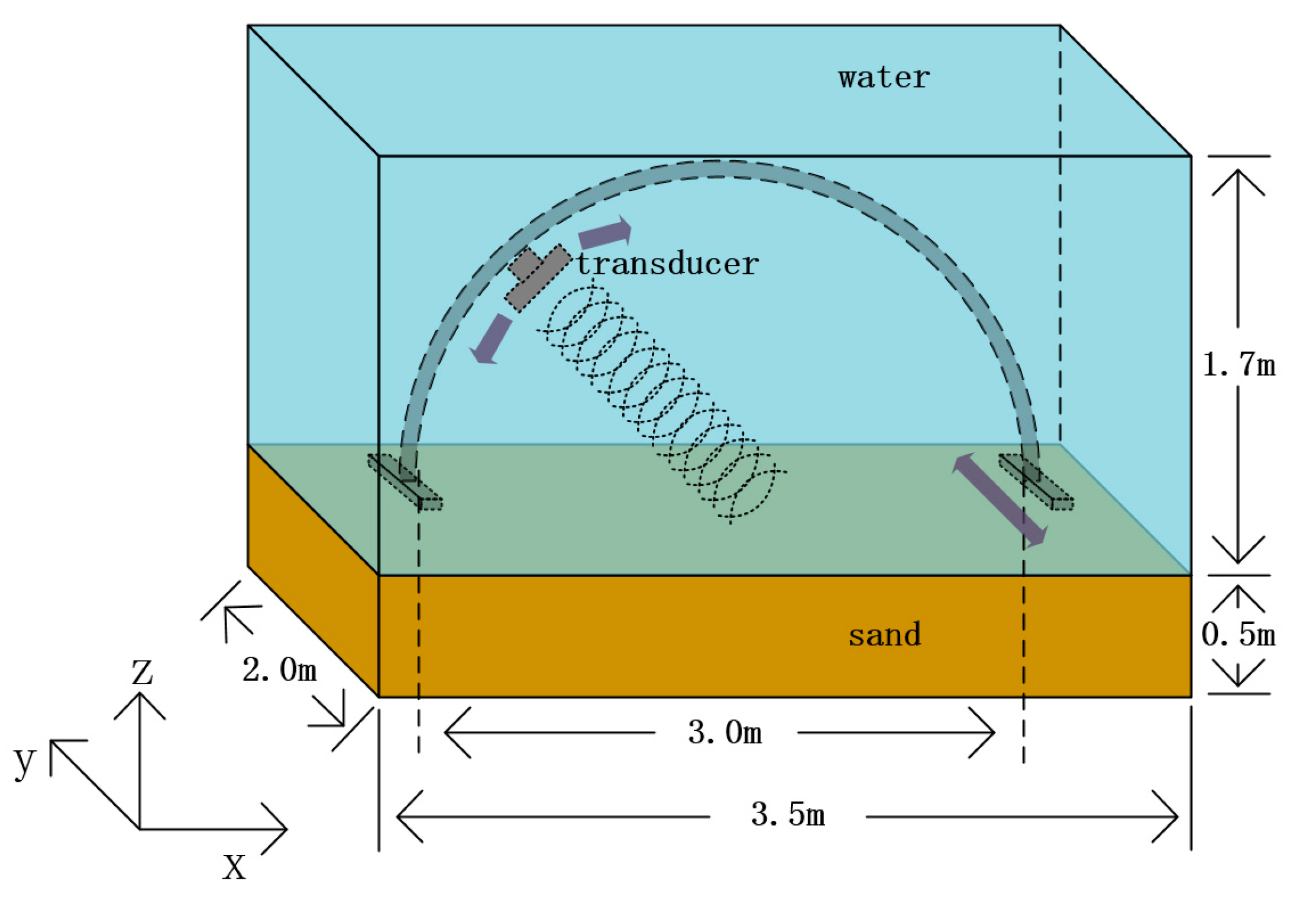
Specialized to the monostatic case, backscattering strength was measured in a rectangular tank using a directional transducer. As shown in Figure 2, a circular arc was used to mount the transducer, and the bottom was filled with river sand. The thickness of the sand layer in the tank was 0.5 m, and the diameter of the circular arc was 3 m. The associated data-processing methods have been described in detail by Jackson [3,62], and only a brief summary of the experimental configuration will be given here. The mean-square voltage at the terminals of the transducer was averaged over groups of 50 successive pings consisting of 10 measurements at five evenly spaced positions in the y direction as the arc moved along the y-axis. This double-averaging was done to mitigate the fluctuation of a single measurement and the potential weak heterogeneity differences of the sand as well as the unevenness of the bottom surface. The transducer was high-frequency broadband, which could move along the arc, and separate passes were made with different grazing angles and frequencies. The grazing angle range and frequencies used in the experiment were 20°–70° and 100 kHz, 120 kHz, and 140 kHz, respectively.
Figure 3 shows measured backscattering strength as a function of grazing angle at different frequencies. It can be seen that the backscattering strength has only a weak frequency dependence. There is a slight drop of backscattering strength above the critical angle of 30° which is consistent with the measurements given by Williams [10]. Although no field experiments were carried out, the authors believe that laboratory measurements are more manageable and provide adequate fitness between model and data. Of course, more subsequent field data for model selection analysis are required due to the limitations of laboratory measurements. This work features the use of a remote sensing scheme with multiple models and lays a foundation for future practical field applications.
4.2. Parameter Inversion
The parameter priors used for the parameter inversion were the same as those for the sensitivity analysis as shown in Table 1 and Table 2. A total of five chains were used during the sampling process and deemed sufficient for parameter dimensions of all models. Under the premise of final convergence, the number of total generations varied between 120,000 and 400,000 depending on the model. The PPDs and Bayes factors were estimated by Equations (51), (52), and (61) using the last 60,000 DREAM samples. Estimates of the one- and two-dimensional marginal PPDs for the three models obtained via Bayesian parameter inversion applied to the backscattering strength data are shown in Figure 4, Figure 5, Figure 6, Figure 7, Figure 8 and Figure 9. The estimates of PPDs for each of the input parameters required by the fluid, grain-shearing elastic, and poroelastic models were obtained by kernel density estimation based on the DREAM samples.
4.2.1. Fluid Model
Figure 4 displays the estimates of one-dimensional marginal PPDs for the fluid model parameters. Inspection of the figure reveals that the roughness spectral exponent , roughness spectral strength , density fluctuation spectral exponent , and porosity were well resolved by the inversion, as their PPDs are much narrower than their respective priors. This is consistent with the results of the sensitivity analysis. The density fluctuation spectral strength , the ratio of compressibility to density fluctuations , the ratio of mass density of grains to water , and the ratio of bulk modulus of grains to water were somewhat resolved by the inversion, as their PPDs changed appreciably from their respective priors. This is not clearly seen in the results of the sensitivity analysis due to its limited resolution. The PPDs of the remaining parameters (mean grain diameter , tortuosity , permeability ) only have a weak peak compared to their priors and provide an unreliable parameter inference.
The two-dimensional characteristics obtained by the inversion of the fluid model are presented in Figure 5, where the two-dimensional marginal PPDs are shown on the top right, and parameter correlations are shown on the bottom left. For intuitive and qualitative understanding, the two-dimensional PPDs have their own color bars, which are not given in the figure. The quantitative correlations are given by the correlation matrix map. The same display applies to the two-dimensional distribution for the next two models. It can be seen that parameter pairs with appreciable positive correlations are as follows: roughness spectral exponent and roughness spectral strength , roughness spectral exponent and porosity , roughness spectral strength and porosity , and the ratio of bulk modulus of grains to water and porosity . Parameter pairs with appreciable negative correlations are the ratio of compressibility to density fluctuations and density fluctuations spectral exponent . Note that parameters with obvious correlation are basically the parameters that are well resolved, as shown in Figure 4. When compared with the roughness spectral exponent , the roughness spectral strength with a relatively low Borgonovo index obtains satisfactory resolution by inversion due to the correlation, and this also appears in the next two inversion results.
4.2.2. Grain-Shearing Elastic Model
Estimates of the one-dimensional marginal PPDs for the grain-shearing elastic model parameters obtained via inversion applied to backscattering strength are shown in Figure 6. We can see by comparing PPDs and priors that the roughness spectral exponent , roughness spectral strength , density fluctuation spectral exponent , and porosity are resolved to a relatively high degree by the inversion. It can be noticed that the resolution of porosity for the grain-shearing elastic model is weaker than that for the fluid model. This could be due to the difference in density ratios used in the two models, as shown in Equations (33) and (17), while sediment mass density is most closely related to porosity. The density fluctuation spectral strength , the ratio of compressibility to density fluctuation , the ratio of mass density of grains to water , the ratio of bulk modulus of grains to water , material exponent , and compressional viscoelastic relaxation time are somewhat resolved by the inversion. The PPDs of the compressional rigidity coefficient and shear rigidity coefficient did not appreciably change from their priors. It is not difficult to find that the results in Figure 6 are consistent with most of the previous results of sensitivity analysis in Figure 1b.
Included in Figure 7 are the estimated two-dimensional marginal PPDs and parameter correlations obtained by the inversion based on the grain-shearing elastic model. From Figure 7 we can see that the parameter correlations of the grain-shearing elastic model are similar to those for the fluid model. In addition, the unique parameter pair of grain-shearing elastic models with appreciable positive correlation is the ratio of bulk modulus of grains to water and material exponent . The parameter pair with appreciable negative correlation is compressional rigidity coefficient and material exponent .
4.2.3. Poroelastic Model
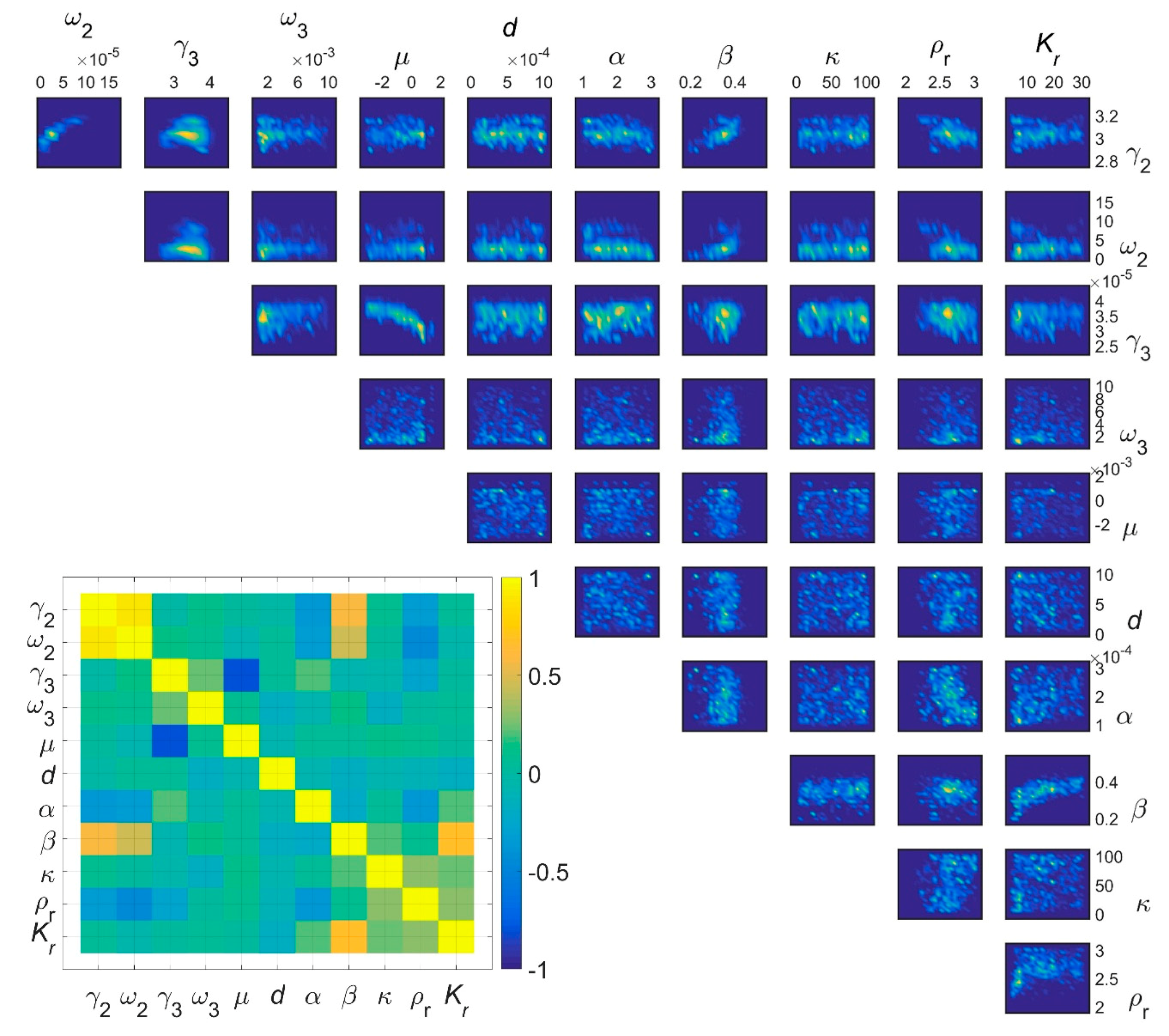
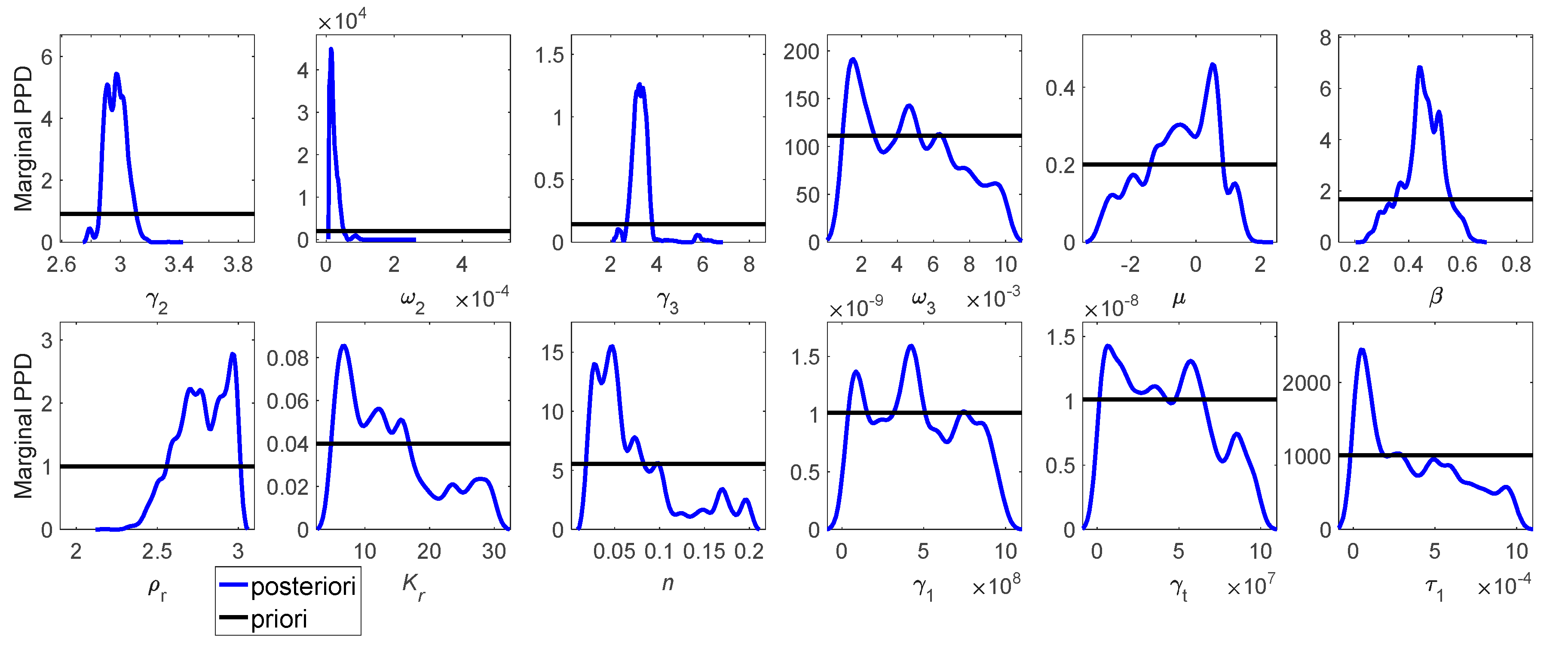
The estimated one-dimensional marginal PPDs for the parameters of the poroelastic model are shown in Figure 8. Comparing the marginal PPDs to their respective priors indicates that the roughness spectral exponent , roughness spectral strength , density fluctuation spectral exponent , ratio of compressibility to density fluctuation , porosity , ratio of mass density of grains to water , ratio of bulk modulus of grains to water , and cementation exponent are well resolved by the inversion. The resolution of porosity of the poroelastic model is similar to that of the grain-shearing elastic model, and this may be due to the same form of density ratio. The density fluctuation spectral strength and high-frequency asymptotic increase are somewhat resolved by the inversion, and the others (mean grain diameter , pore shape factor , Poisson’s ratio of grains , low-frequency asymptotic frame bulk modulus , bulk relaxation frequency ) have unreliable resolutions. The resolutions of the two ratios of the poroelastic model, and , are slightly better than those of the previous two models. The possible reason is that the poroelastic model treats both porosity and elasticity and has inherent advantages for porous mediums such as sandy sediments, for which it is possible that the fluid and granular phases will vibrate differently in response to acoustic excitation [3]. From a mathematical perspective, the two parameters can be more coupled with the scattering strength, as shown by the equations in Appendix B. The resolutions of interface roughness parameters (roughness spectral exponent , roughness spectral strength ) and volume inhomogeneity parameters (density fluctuation spectral exponent , density fluctuation spectral strength , ratio of compressibility to density fluctuations ) of the three models have a certain degree of difference, while the common parameters of the poroelastic model have slightly better resolution in general. Compared with the previous sensitivity analysis results in Figure 1c, the results here show better resolution and have more information about model parameters. Despite the total number of model parameters and the number of parameters that are somewhat resolved, the inversion based on the poroelastic model provides four more well-resolved parameters than that based on the other two models. The resolutions of common parameters of the poroelastic model are also slightly better than that of the other two models. From the perspective of the PPDs of the model parameters, more reliable information of sediment properties is provided by the inversion based on the poroelastic model, which can be considered superior to the other two models.
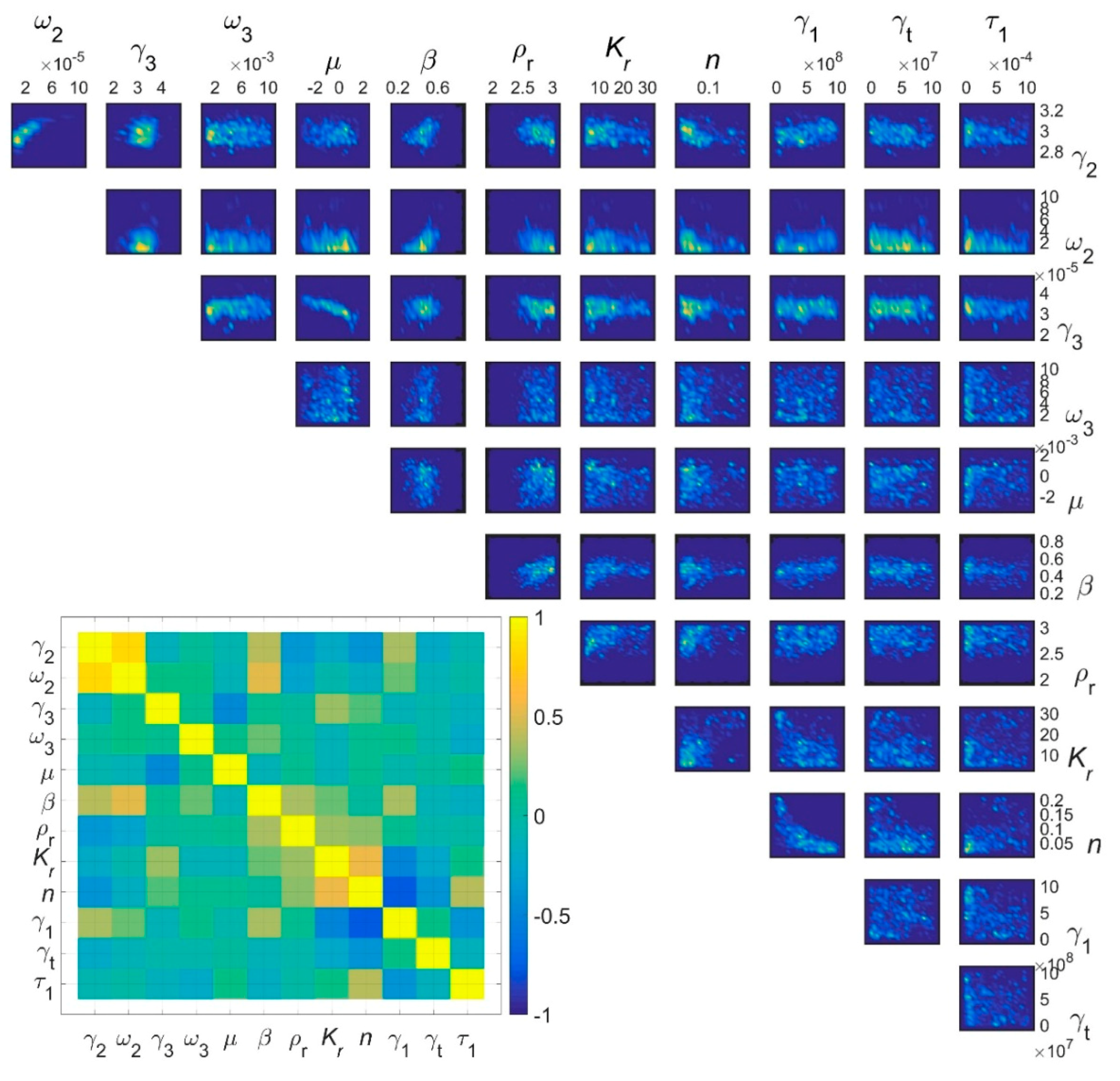
Figure 9 shows the estimates of two-dimensional marginal PPDs and parameter correlations obtained by the inversion based on the poroelastic model. In addition to the parameter correlations similar to the fluid model, the parameter pair, which is the ratio of bulk modulus of grains to water and cementation exponent , has an appreciable positive correlation. It should be viewed with caution that these correlations are only shown by the samples, and not all of them have practical physical meaning. The same attention needs to be paid to the two-dimensional marginal PPDs of the previous two models. Indeed, it is difficult to provide a physical reason for the parameter correlations shown by the inversion results, as part of them cannot be measured by any means. The authors believe that the universality of these correlations needs to be further verified and analyzed by model-based inversions using additional measurements for different types of sandy sediments. Taking available sediment properties measured in situ as intermediate quantities of parameter pairs with correlations may help explain the correlations.
4.3. Model Comparison and Selection
The model comparison and selection results obtained by the inversion using backscattering strength data are shown in Figure 10, Figure 11 and Figure 12. Figure 10 gives a comparison of the uncertainties of the ratios of compressional and shear sound speed in sediment to compressional sound speed in water. The uncertainties of attenuation of the two types of sound waves are also shown in Figure 10. The sets of estimated sound speed ratios and attenuation at different frequencies are calculated by the samples with the three geoacoustic models, EDFM, VGS(), and CREB. The PPDs of sound speed ratio and attenuation are also obtained by kernel density estimation based on the estimated sets. Because of the finite number of three frequencies, the frequency dependences for sound speed and attenuation are not obvious in these results. Comparing the PPDs of compressional wave indicates that the predicted uncertainties of CREB are slightly more concentrated than those of EDFM and their maximum posterior estimates are very close to each other, as shown in the left side of Figure 10. The PPDs of the compressional wave of EDFM and CREB have a slight sound speed ratio difference and an appreciable attenuation difference compared to VGS(). This suggests that the scattering strengths of the fluid and poroelastic models are more sensitive to attenuation than the grain-shearing elastic model. Besides, the scattering strengths of the three models are much more sensitive to compressional sound speed than attenuation as the PPDs of compressional speed ratio are all highly concentrated.
From the right side of Figure 10, it can be seen that shear sound speed predicted by CREB is larger than that predicted by VGS() and the uncertainties of attenuation are roughly similar. Compared with compressional sound speed, the shear sound speed in sandy sediments is much lower. This suggests that the addition of shear waves is only a minor modification to model the scattering strength [3] and the uncertainty of shear sound speed is larger than that of compressional sound speed. Since slow compressional waves supported in a poroelastic medium are given theoretically and have never been observed in natural marine sediment, the uncertainties of sound speed and attenuation for slow compressional waves are not given here.
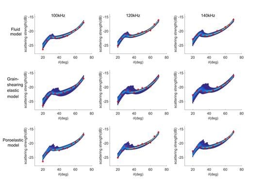
Figure 11 depicts a comparison of the uncertainties of backscattering strength predicted by the samples. The DREAM samples were substituted into each model to calculate the estimated backscattering strength set at different frequencies and angles. For a selected model at a selected frequency, the estimated backscattering strength set at each angle was statistically transformed into a probability distribution, which is represented by a vertical color strip. All the vertical color strips for the whole angle range were spliced together along the x-axis to form the subgraphs in Figure 11. Experimental measurements are also shown in the figure. In general, all three models are well matched with the experimental measurements. Appreciable differences of uncertainties of the estimated backscattering strength for the three models can be seen in Figure 11, and the fluid model has the most concentrated posterior predictive distributions. The results of the fluid model are only slightly different from those of the poroelastic model near the critical angle. Compared with the fluid and poroelastic models, the results for the grain-shearing elastic model have the greatest uncertainties and smallest concentration. The fluid model seemingly does the best job of matching the frequency and angle dependence of the backscattering strength data for sandy sediments. Comparing Figure 10 and Figure 11, it can also be seen that differences of uncertainties of the estimated backscattering strength correspond to the differences of uncertainties of the estimated sound speed and attenuation for the three models. The fluid and poroelastic models are similar, and they both have appreciable differences compared with the grain-shearing elastic model.
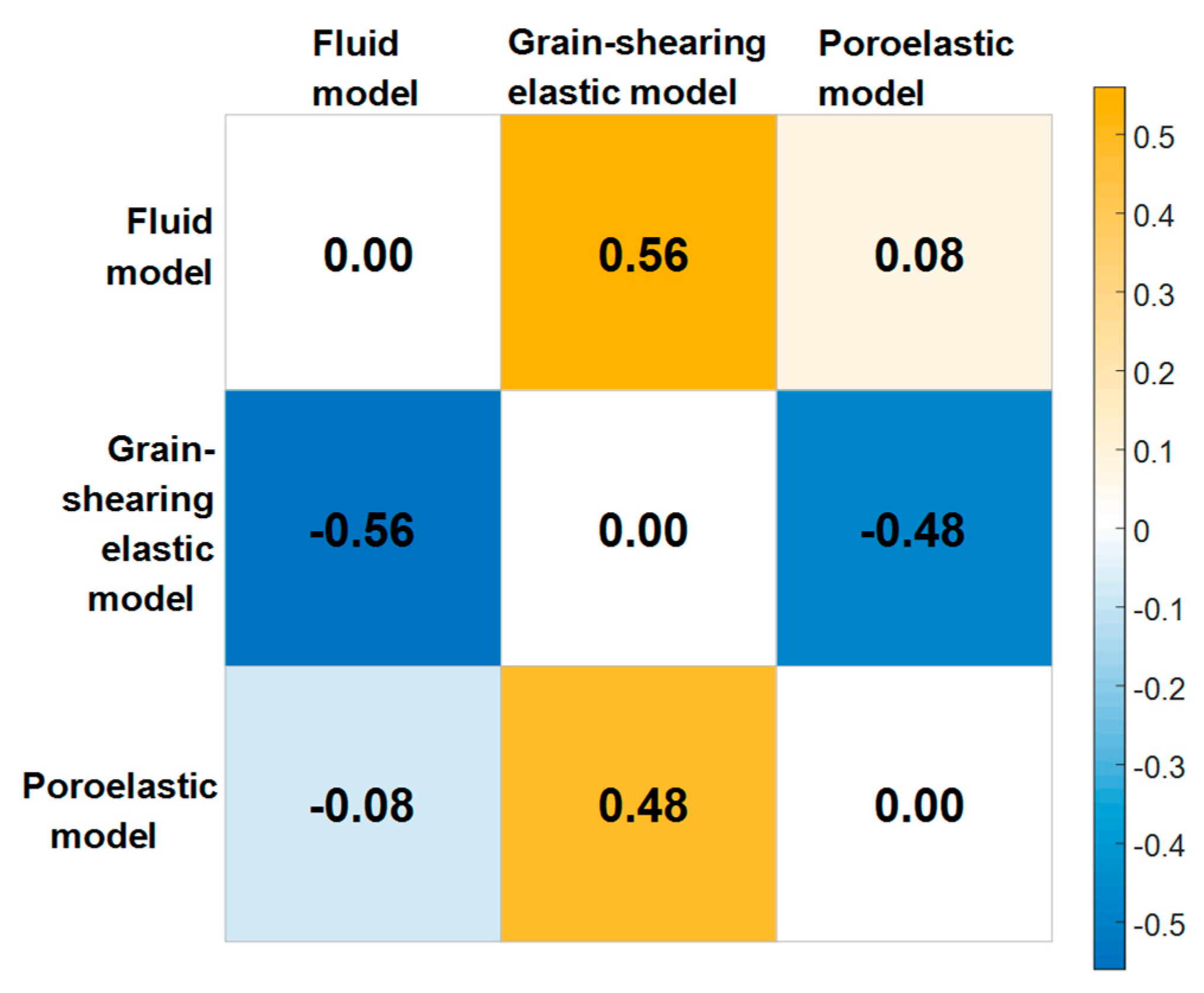
The comparison of Bayes factors of different model pairs obtained by the inversion based on the backscattering strength data is summarized in Figure 12. Referring to the factor scale given in Table 3, the evidence in favor of the fluid model over the grain-shearing elastic model can be considered substantial. The Bayesian evidence for the fluid and poroelastic models is similar, with the fluid model slightly favored. This similarity and the similarity of compressional sound speed and attenuation, as shown in Figure 10, can be understood since the EDFM used in the fluid model is essentially an approximation of the full Biot–Stoll model and the corrected and reparametrized extended Biot–Stoll model is used in the poroelastic model. It has been proven that backscattering strength, compressional sound speed, and attenuation predicted by the fluid model based on the EDFM are very close to the predictions of full Biot–Stoll theory for sandy sediment [10,12,19]. The poroelastic model, which takes sediment composed of grains and water as a two-phase system, is essentially the most reasonable approximation for sandy sediments. In this sense, the poroelastic and fluid models are both superior to the grain-shearing elastic model. Although the Bayes factors show slight differences between the fluid and poroelastic models, we still consider the poroelastic model to be the best because the inversion based on the poroelastic model provides the best-resolved parameters, as discussed in Section 4.2.3.
5. Conclusions
Based on the combination of geoacoustic models and corresponding scattering models, Bayesian inversion and model selection techniques are applied to compare three sediment acoustic models: the fluid model with EDFM, the grain-shearing elastic model with VGS(λ), and the poroelastic model with CREB. The combination allows us to use backscattering strength measured remotely to carry out the parameter inversions. Parameter uncertainties are given by the one- and two-dimensional PPDs estimated by the DREAM samples.
Two studies were carried out using the inversion results. First, the resolution and correlation of parameters for the three models were compared based on the estimates of PPDs. The poroelastic model provides more well-resolved parameters than the other two models. In general, the resolutions of common parameters of the poroelastic model are also slightly better than those of the other two models. In other words, the inversion based on the poroelastic model can provide more highly resolved information about sediments properties, some of which are difficult to measure directly.
The second study involved model comparison and selection using model predictions and Bayes factors. Based on the DREAM samples, the predictions using different models and acoustic frequencies were calculated for qualitative comparative analysis with the backscattering strength measurements, and the Bayes factors of the three models are calculated for quantitative comparison. From the analysis, it appears that all three models can produce predictions that agree with the measurements, though the fluid and poroelastic models appear to outperform the grain-shearing elastic model. It should be viewed with caution that the model comparison results are obtained by the inversion based only on the limited measurements of sandy sediments. Indeed, the effectiveness of the poroelastic model for sandy sediments has been authenticated and is noticeable.
The results in this paper indicate that the best model for sandy sediments is the poroelastic model. However, it has been suggested that the elastic model presumably is better for softer sediments than the poroelastic model. Besides, the interface roughness scattering model that accommodates shear can provide an appreciable correction to the fluid model for consolidated sediments such as rock seafloor, which has a greater shear wave speed than the sound speed in water. Much attention has been paid to model sound propagation in sandy sediments, and no single model can be applied to all types of sediment. Despite its importance, this topic has largely been ignored in the literature to date. We have performed a comparative study of evidence estimation for the remote sensing of sediment properties in this paper. This was an attempt to implement a combination of several different models for geoacoustic inversion, and the model that best matches the measurements was obtained. The attempt provides a relatively feasible remote sensing scheme for various types of sediments under unknown conditions. However, this scheme should be regarded as tentative and requires more measurements of different types of sediment for validation.
Author Contributions
Conceptualization, B.Z. and J.Z.; data curation, B.Z., Z.Q., and Z.L.; funding acquisition, J.Z.; investigation, B.Z.; methodology, B.Z.; project administration, J.Z.; validation, B.Z., Z.Q., and Z.L.; writing—original draft, B.Z.; writing—review and editing, J.Z.
Funding
This study was supported by the National Key Research and Development Program of China (nos. 2016YFC1401203, 2018YFC1407400).
Acknowledgments
Thanks are due to Jian Xu and Bin Xue for providing the experimental instruments and to Haihan Zhao for assistance in the experiment. The authors would also like to thank the anonymous reviewers for their constructive comments and suggestions.
Conflicts of Interest
The authors declare no conflict of interest.
Appendix A
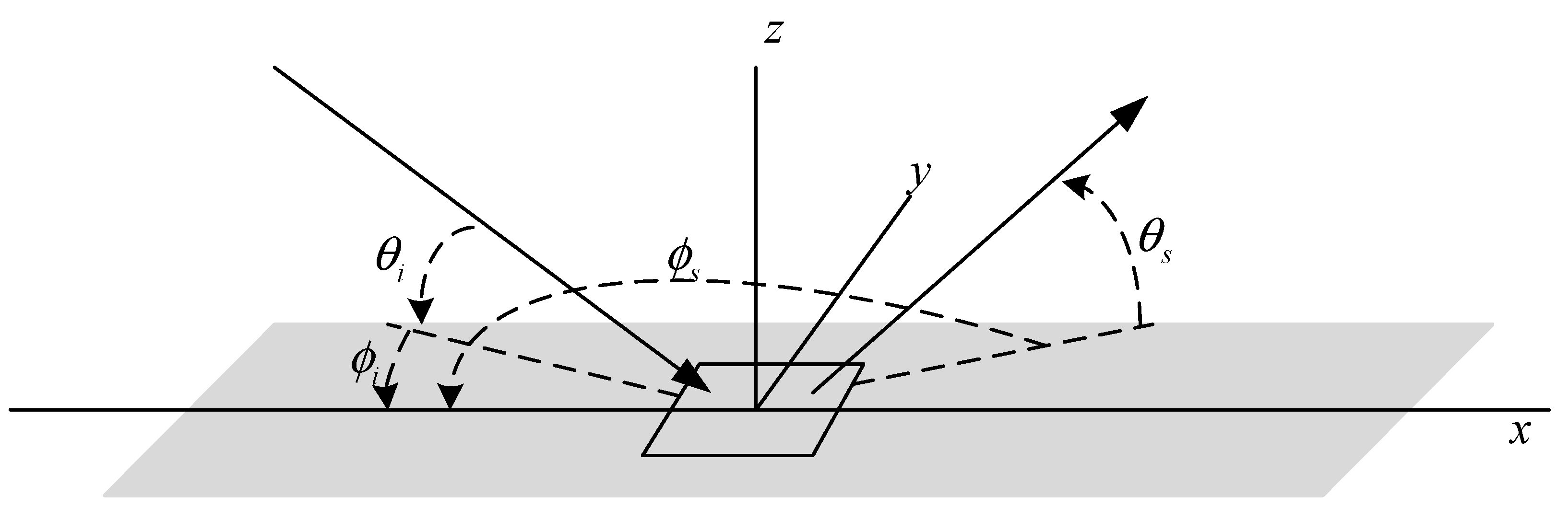
Figure A1.
Definition of angle of incident and scattered waves.

The in-water wave vectors of incident and scattered directions are defined as follows [63]:
where is the acoustic wavenumber in water. and are speed of sound in water and acoustic frequency, respectively. It is noted that one may set without loss of generality if the seafloor is isotropic in the statistical sense. The horizontal components and vertical component of the above wave vectors respectively are
where the uppercase, boldface symbols represent the horizontal components. The following wave vector differences needed in the model calculation are defined:
Based on the Snell’s law, the wave vectors for the incident and scattered compressional waves in the sediment are
where is the acoustic complex speed ratio. Then, the real part of the vector difference of the scattered and incident waves that propagate in sediment is
The magnitude of a difference vector is denoted without boldface in the paper. we may set , for backscatter.
Appendix B
The needed quantities for the elastic interface roughness scattering model are given by the following expressions [3]:
where and the complex cosines needed are obtained by
The needed quantities for the poroelastic interface roughness scattering model are given by the following expressions [39]:
where the vertical line in Equation (A20) separates it into the matrices, , and the column matrices, . The elements of and are:
where . is the Kronecker delta, is the spatial components (x, y, z) of vector . The expressions of and are
References
- Anderson, J.T.; Van Holliday, D.; Kloser, R.; Reid, D.G.; Simard, Y. Acoustic seabed classification: Current practice and future directions. ICES J. Mar. Sci. 2008, 65, 1004–1011. [Google Scholar] [CrossRef]
- Siemes, K.; Hermand, J.P.; Snellen, M.; Simons, D.G. Toward an Efficient and Comprehensive Assessment of Marine Sediments through Combining Hydrographic Surveying and Geoacoustic Inversion. IEEE J. Ocean. Eng. 2016, 41, 190–203. [Google Scholar]
- Jackson, D.R.; Richardson, M.D. High-Frequency Seafloor Acoustics; Springer: New York, NY, USA, 2007. [Google Scholar]
- Chotiros, N.P.; Isakson, M.J. A broadband model of sandy ocean sediments: Biot–Stoll with contact squirt flow and shear drag. J. Acoust. Soc. Am. 2004, 116, 2011–2022. [Google Scholar] [CrossRef]
- Buckingham, M.J. Compressional and shear wave properties of marine sediments: Comparisons between theory and data. J. Acoust. Soc. Am. 2005, 117, 137–152. [Google Scholar] [CrossRef] [PubMed]
- Buckingham, M.J. On pore-fluid viscosity and the wave properties of saturated granular materials including marine sediments. J. Acoust. Soc. Am. 2007, 122, 1486. [Google Scholar] [CrossRef] [PubMed]
- Williams, K.L. Adding thermal and granularity effects to the effective density fluid model. J. Acoust. Soc. Am. 2013, 133, EL431–EL437. [Google Scholar] [CrossRef] [PubMed]
- Buckingham, M.J. Analysis of shear-wave attenuation in unconsolidated sands and glass beads. J. Acoust. Soc. Am. 2014, 136, 2478–2488. [Google Scholar] [CrossRef] [PubMed]
- Chotiros, N.P.; Isakson, M.J. Shear wave attenuation and micro-fluidics in water-saturated sand and glass beads. J. Acoust. Soc. Am. 2014, 135, 3264–3279. [Google Scholar] [CrossRef] [PubMed]
- Williams, K.L.; Jackson, D.R.; Thorsos, E.I.; Tang, D.J.; Briggs, K.B. Acoustic backscattering experiments in a well characterized sand sediment: Data/model comparisons using sediment fluid and Biot models. IEEE J. Ocean. Eng. 2002, 27, 376–387. [Google Scholar] [CrossRef]
- Ohkawa, K.; Yamaoka, H.; Yamamoto, T. Acoustic backscattering from a sandy seabed. IEEE J. Ocean. Eng. 2005, 30, 700–708. [Google Scholar] [CrossRef]
- Williams, K.L.; Jackson, D.R.; Dajun, T.; Briggs, K.B.; Thorsos, E.I. Acoustic Backscattering From a Sand and a Sand/Mud Environment: Experiments and Data/Model Comparisons. IEEE J. Ocean. Eng. 2009, 34, 388–398. [Google Scholar] [CrossRef]
- Williams, K.L.; Thorsos, E.I.; Jackson, D.R.; Hefner, B.T. Thirty years of sand acoustics: A perspective on experiments, models and data/model comparisons. AIP Conf. Proc. 2012, 1495, 166–192. [Google Scholar]
- Biot, M. Theory of Propagation of Elastic Waves in a Fluid-Saturated Porous Solid. I. Low-Frequency Range. J. Acoust. Soc. Am. 1956, 28, 168–178. [Google Scholar] [CrossRef]
- Biot, M. Theory of Propagation of Elastic Waves in a Fluid-Saturated Porous Solid. II. Higher Frequency Range. Acoust. Soc. Am. J. 1956, 28, 179–191. [Google Scholar] [CrossRef]
- Stoll, R.D. Sediment Acoustics. Lecture Notes in Earth Sciences; Springer: Berlin, Germany, 1989; pp. 1–101. [Google Scholar]
- Chotiros, N.P. Acoustics of the Seabed as a Poroelastic Medium; Springer: Berlin/Heidelberg, Germany, 2017. [Google Scholar]
- Bonomo, A.L.; Isakson, M.J. A comparison of three geoacoustic models using Bayesian inversion and selection techniques applied to wave speed and attenuation measurements. J. Acoust. Soc. Am. 2018, 143, 2501. [Google Scholar] [CrossRef] [PubMed]
- Williams, K.L. An effective density fluid model for acoustic propagation in sediments derived from Biot theory. J. Acoust. Soc. Am. 2001, 110, 2276–2281. [Google Scholar] [CrossRef] [PubMed]
- Williams, K.L.; Jackson, D.R.; Thorsos, E.I.; Dajun, T.; Schock, S.G. Comparison of sound speed and attenuation measured in a sandy sediment to predictions based on the Biot theory of porous media. IEEE J. Ocean. Eng. 2002, 27, 413–428. [Google Scholar] [CrossRef]
- Bonomo, A.L.; Chotiros, N.P.; Isakson, M.J. On the validity of the effective density fluid model as an approximation of a poroelastic sediment layer. J. Acoust. Soc. Am. 2015, 138, 748–757. [Google Scholar] [CrossRef] [PubMed] [Green Version]
- Buckingham, M.J. Wave propagation, stress relaxation, and grain-to-grain shearing in saturated, unconsolidated marine sediments. J. Acoust. Soc. Am. 2000, 108, 2796–2815. [Google Scholar] [CrossRef]
- Buckingham, M.J. Response to “Comments on ‘Pore fluid viscosity and the wave properties of saturated granular materials including marine sediments [J. Acoust. Soc. Am. 127, 2095–2098 (2010)]’”. J. Acoust. Soc. Am. 2010, 127, 2099. [Google Scholar] [CrossRef]
- Dettmer, J.; Dosso, S.E.; Holland, C.W. Model selection and Bayesian inference for high-resolution seabed reflection inversion. J. Acoust. Soc. Am. 2009, 125, 706–716. [Google Scholar] [CrossRef]
- Dosso, S.E.; Nielsen, P.L.; Harrison, C.H. Bayesian inversion of reverberation and propagation data for geoacoustic and scattering parameters. J. Acoust. Soc. Am. 2009, 125, 2867–2880. [Google Scholar] [CrossRef] [PubMed]
- Dosso, S.E.; Dettmer, J.; Steininger, G.; Holland, C.W. Efficient trans-dimensional Bayesian inversion for geoacoustic profile estimation. Inverse Probl. 2014, 30, 114018. [Google Scholar] [CrossRef]
- Simons, D.G.; Snellen, M. A Bayesian approach to seafloor classification using multi-beam echo-sounder backscatter data. Appl. Acoust. 2009, 70, 1258–1268. [Google Scholar] [CrossRef]
- Landmark, K.; Solberg, A.H.S.; Austeng, A.; Hansen, R.E. Bayesian Seabed Classification Using Angle-Dependent Backscatter Data From Multibeam Echo Sounders. IEEE J. Ocean. Eng. 2014, 39, 724–739. [Google Scholar] [CrossRef]
- Bourbie, T.; Coussy, O.; Zinszner, B. Acoustics of Porous Media; Editions Technip: Paris, France, 1987. [Google Scholar]
- Stoll, R.D. Acoustic Waves in Saturated Sediments; Springer: Boston, MA, USA, 1974. [Google Scholar]
- Zou, D.P.; Williams, K.L.; Thorsos, E.I. Influence of Temperature on Acoustic Sound Speed and Attenuation of Seafloor Sand Sediment. IEEE J. Ocean. Eng. 2015, 40, 969–980. [Google Scholar]
- Thorsos, E.I.; Jackson, D.R. The validity of the perturbation approximation for rough surface scattering using a Gaussian roughness spectrum. J. Acoust. Soc. Am. 1989, 86, 261–277. [Google Scholar] [CrossRef]
- Thorsos, E.I. The Validity of the Kirchoff Approximation for Rough Surface Scattering Using a Gaussian Roughness Spectrum. J. Acoust. Soc. Am. 1998, 86 (Suppl. 1), 20. [Google Scholar]
- Voronovich, A. Small-slope approximation in wave scattering by rough surfaces. Sov. Phys. JETP 1985, 62, 65–70. [Google Scholar]
- Williams, K.L.; Jackson, D.R. Bistatic bottom scattering: Model, experiments, and model/data comparison. J. Acoust. Soc. Am. 1998, 103, 169–181. [Google Scholar] [CrossRef]
- Pouliquen, E.; Lyons, A.P.; Pace, N.G. Penetration of acoustic waves into rippled sandy seafloors. J. Acoust. Soc. Am. 2000, 1 Pt 1, 2071–2081. [Google Scholar] [CrossRef]
- Hamilton, E.L. Elastic properties of marine sediments. J. Geophys. Res. 1971, 76, 579–604. [Google Scholar] [CrossRef]
- Hamilton, E.L.; Bachman, R.T. Sound velocity and related properties of marine sediments. J. Acoust. Soc. Am. 1982, 72, 1891–1904. [Google Scholar] [CrossRef]
- Williams, K.L.; Grochocinski, J.M.; Jackson, D.R. Interface scattering by poroelastic seafloors: First-order theory. J. Acoust. Soc. Am. 2001, 110, 2956–2963. [Google Scholar] [CrossRef]
- Borgonovo, E. A new uncertainty importance measure. Reliab. Eng. Syst. Saf. 2007, 92, 771–784. [Google Scholar] [CrossRef]
- Sobol, I.M. Theorems and examples on high dimensional model representation. Reliab. Eng. Syst. Saf. 2003, 79, 187–193. [Google Scholar] [CrossRef]
- Sobol, I.M. Global sensitivity indices for nonlinear mathematical models and their Monte Carlo estimates. Math. Comput. Simul. 2001, 55, 271–280. [Google Scholar] [CrossRef]
- Saltelli, A.; Tarantola, S.; Campolongo, F. Sensitivity anaysis as an ingredient of modeling. Stat. Sci. 2000, 15, 377–395. [Google Scholar]
- Rabitz, H.; Aliş, Ö.F. General foundations of high-dimensional model representations. J. Math. Chem. 1999, 25, 197–233. [Google Scholar] [CrossRef]
- Hefner, B.T.; Williams, K.L. Sound speed and attenuation measurements in unconsolidated glass-bead sediments saturated with viscous pore fluids. J. Acoust. Soc. Am. 2006, 120, 2538–2549. [Google Scholar] [CrossRef]
- Helton, J.C.; Davis, F.J. Latin hypercube sampling and the propagation of uncertainty in analyses of complex systems. Reliab. Eng. Syst. Saf. 2003, 81, 23–69. [Google Scholar] [CrossRef] [Green Version]
- Dosso, S.E. Quantifying uncertainty in geoacoustic inversion. I. A fast Gibbs sampler approach. J. Acoust. Soc. Am. 2002, 111, 129–142. [Google Scholar] [CrossRef] [PubMed]
- Dosso, S.E.; Dettmer, J. Bayesian matched-field geoacoustic inversion. Inverse Probl. 2011, 27, 055009. [Google Scholar] [CrossRef] [Green Version]
- Yang, K.D.; Xiao, P.; Duan, R.; Ma, Y.L. Bayesian Inversion for Geoacoustic Parameters from Ocean Bottom Reflection Loss. J. Comput. Acoust. 2017, 25. [Google Scholar] [CrossRef]
- Hastings, W.K. Monte Carlo Sampling Methods Using Markov Chains and Their Applications. Biometrika 1970, 57, 97. [Google Scholar] [CrossRef]
- Haario, H.; Saksman, E.; Tamminen, J. Adaptive proposal distribution for random walk Metropolis algorithm. Comput. Stat. 1999, 14, 375–395. [Google Scholar] [CrossRef]
- Haario, H.; Saksman, E.; Tamminen, J. An adaptive Metropolis algorithm. Bernoulli 2001, 7, 223–242. [Google Scholar] [CrossRef]
- Haario, H.; Laine, M.; Mira, A.; Saksman, E. DRAM: Efficient adaptive MCMC. Stat. Comput. 2006, 16, 339–354. [Google Scholar] [CrossRef] [Green Version]
- Braak, C.J.F.T. A Markov Chain Monte Carlo version of the genetic algorithm Differential Evolution: Easy Bayesian computing for real parameter spaces. Stat. Comput. 2006, 16, 239–249. [Google Scholar] [CrossRef]
- Vrugt, J.A.; Braak, C.J.F.T.; Diks, C.G.H.; Robinson, B.A.; Hyman, J.M.; Higdon, D. Accelerating Markov Chain Monte Carlo Simulation by Differential Evolution with Self-Adaptive Randomized Subspace Sampling. Int. J. Nonlinear Sci. Numer. Simul. 2009, 10, 273–290. [Google Scholar] [CrossRef] [Green Version]
- Dosso, S.E.; Nielsen, P.L. Quantifying uncertainty in geoacoustic inversion. II. Application to broadband, shallow-water data. J. Acoust. Soc. Am. 2002, 111, 143–159. [Google Scholar] [CrossRef] [PubMed]
- Vrugt, J.A. Markov chain Monte Carlo simulation using the DREAM software package: Theory, concepts, and MATLAB implementation. Environ. Model. Softw. 2016, 75, 273–316. [Google Scholar] [CrossRef] [Green Version]
- Gelman, A.; Rubin, D.B. Inference from Iterative Simulation Using Multiple Sequences. Stat. Sci. 1992, 7, 457–472. [Google Scholar] [CrossRef]
- Brooks, S.P.; Gelman, A. General methods for monitoring convergence of iterative simulations. J. Comput. Graph. Stat. 1998, 7, 434–455. [Google Scholar]
- Kass, R.E.; Raftery, A.E. Bayes Factors. J. Am. Stat. Assoc. 1995, 90, 773–795. [Google Scholar] [CrossRef]
- Brunetti, C.; Linde, N.; Vrugt, J.A. Bayesian model selection in hydrogeophysics: Application to conceptual subsurface models of the South Oyster Bacterial Transport Site, Virginia, USA. Adv. Water Resour. 2017, 102, 127–141. [Google Scholar] [CrossRef] [Green Version]
- Jackson, D.R.; Baird, A.M.; Crisp, J.J.; Thomson, P.A.G. High-frequency bottom backscatter measurements in shallow water. J. Acoust. Soc. Am. 1986, 80, 1188–1199. [Google Scholar] [CrossRef]
- Zou, B.; Zhai, J.; Xu, J.; Li, Z.; Gao, S. A Method for Estimating Dominant Acoustic Backscatter Mechanism of Water-Seabed Interface via Relative Entropy Estimation. Math. Probl. Eng. 2018, 2018, 10. [Google Scholar] [CrossRef]
Figure 1.
Borgonovo indices for: (a) fluid model; (b) grain-shearing elastic model; (c) poroelastic model.
Figure 1.
Borgonovo indices for: (a) fluid model; (b) grain-shearing elastic model; (c) poroelastic model.

Figure 2.
Diagram of backscatter measurements.

Figure 3.
Measured backscattering strength as a function of grazing angle of different frequencies.
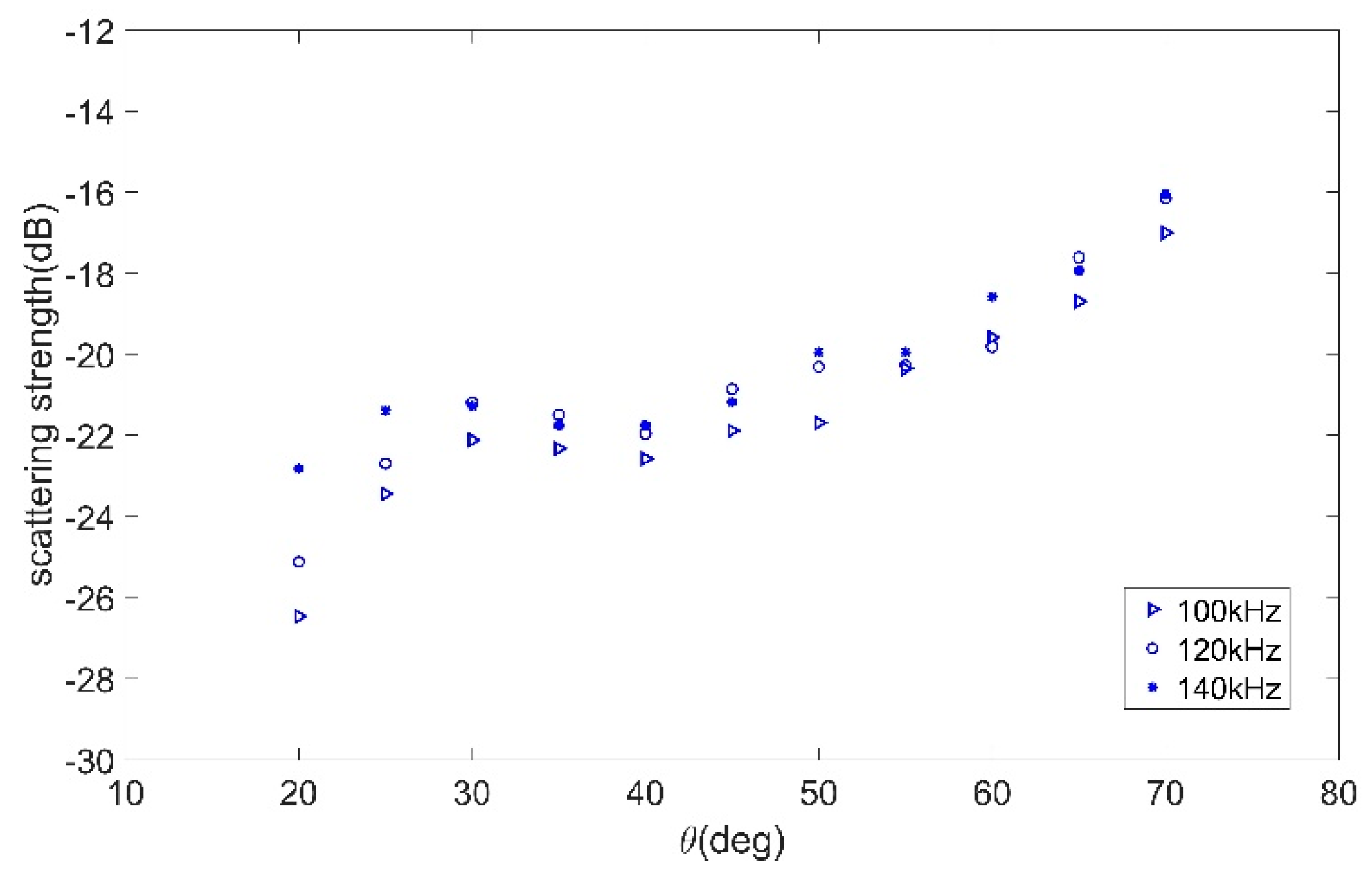
Figure 4.
Estimates of one-dimensional marginal posterior probability distributions (PPDs) for fluid model parameters.
Figure 4.
Estimates of one-dimensional marginal posterior probability distributions (PPDs) for fluid model parameters.
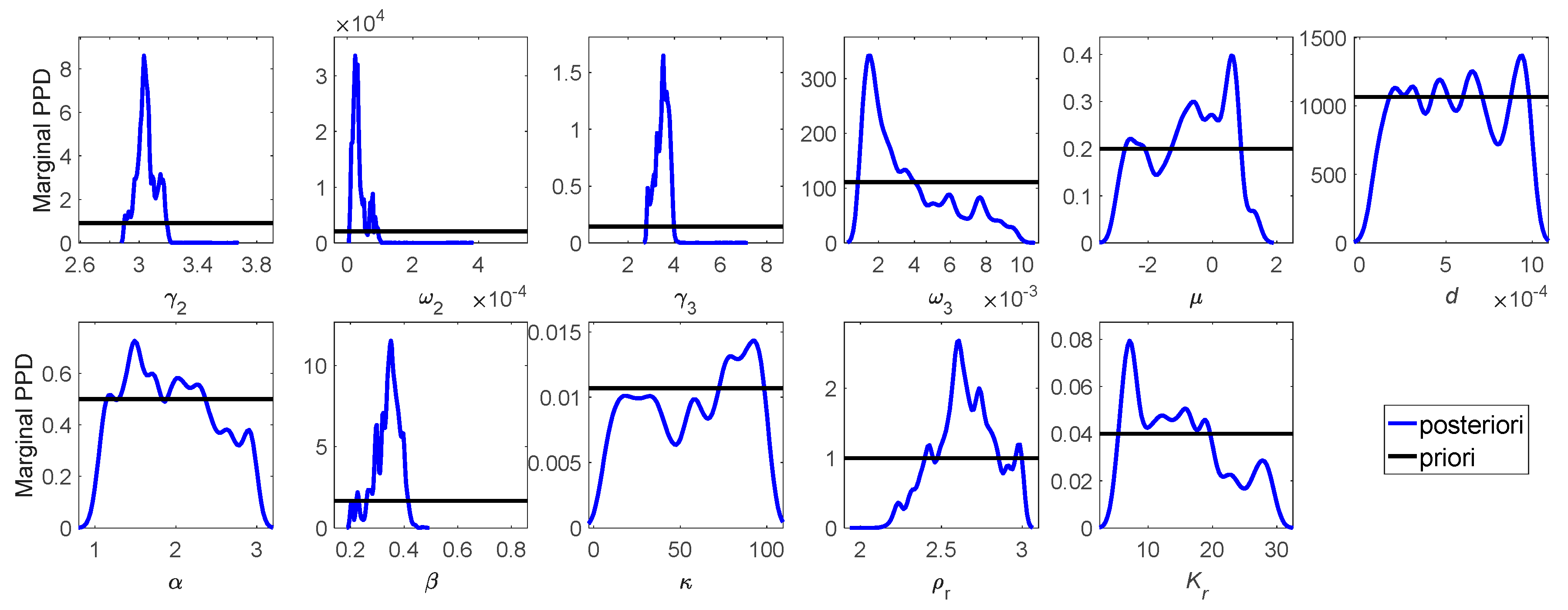
Figure 5.
Estimates of two-dimensional marginal PPDs for fluid model parameters (top right) and correlation matrix map (bottom left).
Figure 5.
Estimates of two-dimensional marginal PPDs for fluid model parameters (top right) and correlation matrix map (bottom left).

Figure 6.
Estimates of one-dimensional marginal PPDs for grain-shearing elastic model parameters.

Figure 7.
Estimates of two-dimensional marginal PPDs for grain-shearing elastic model parameters (top right) and correlation matrix map (bottom left).
Figure 7.
Estimates of two-dimensional marginal PPDs for grain-shearing elastic model parameters (top right) and correlation matrix map (bottom left).

Figure 8.
Estimates of one-dimensional marginal PPDs for poroelastic model parameters.
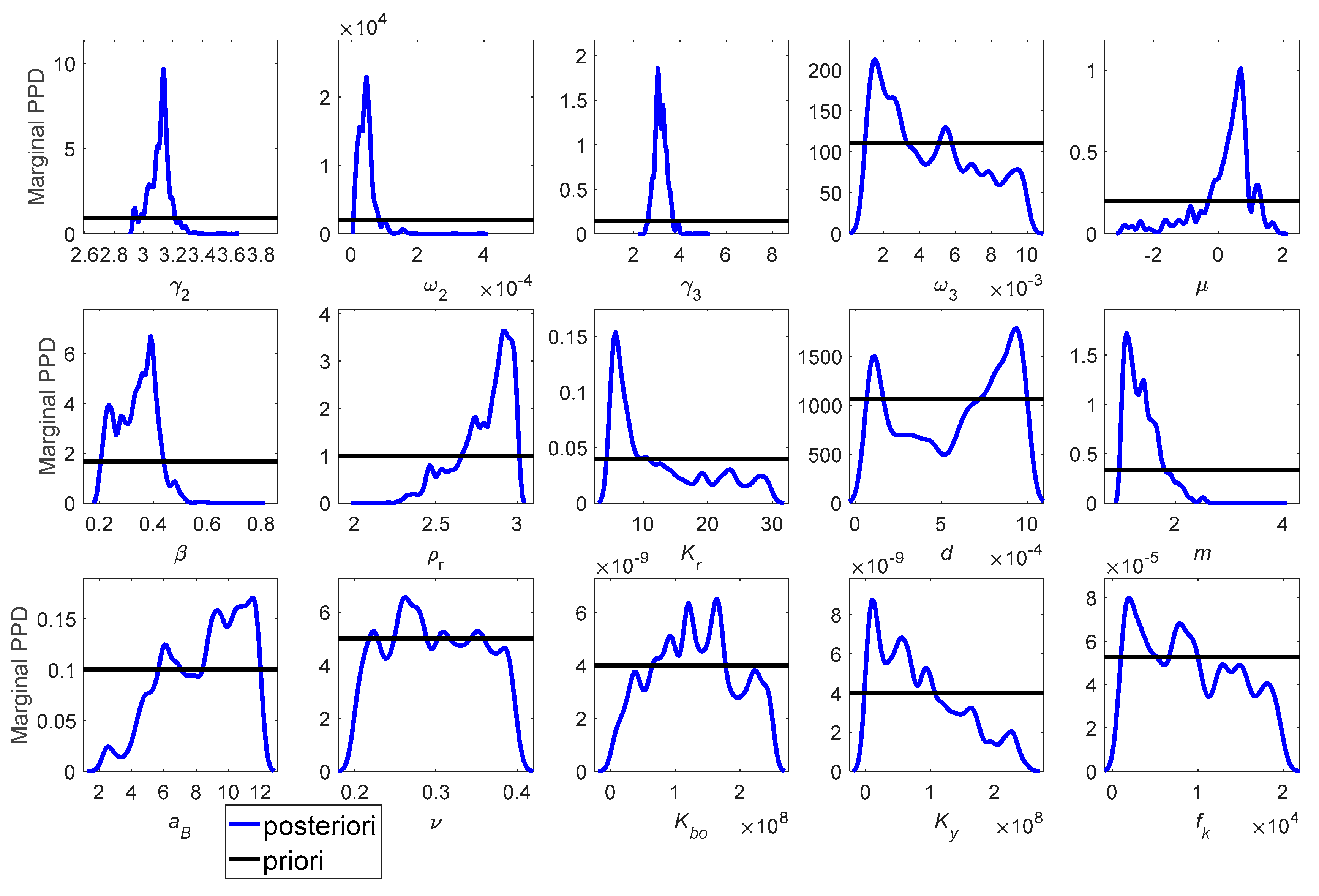
Figure 9.
Estimates of two-dimensional marginal PPDs for poroelastic model parameters (top right) and correlation matrix map (bottom left).
Figure 9.
Estimates of two-dimensional marginal PPDs for poroelastic model parameters (top right) and correlation matrix map (bottom left).
Figure 10.
Comparison of uncertainties of ratios of compressional and shear sound speed in sediment to compressional sound speed in water and corresponding attenuation.
Figure 10.
Comparison of uncertainties of ratios of compressional and shear sound speed in sediment to compressional sound speed in water and corresponding attenuation.
Figure 11.
Comparison of uncertainties of backscattering strength predicted by samples based on different models and acoustic frequencies. Red asterisks represent corresponding experimental measurements, as shown in Figure 3.
Figure 11.
Comparison of uncertainties of backscattering strength predicted by samples based on different models and acoustic frequencies. Red asterisks represent corresponding experimental measurements, as shown in Figure 3.
Figure 12.
Comparison of Bayes factors calculated for each pair of models through Bayesian inference applied to backscattering strength data. Number superimposed over each matrix element is the base 10 logarithm of the Bayes factor for a given pair of models.
Figure 12.
Comparison of Bayes factors calculated for each pair of models through Bayesian inference applied to backscattering strength data. Number superimposed over each matrix element is the base 10 logarithm of the Bayes factor for a given pair of models.


Table 1.
Parameter bounds used to construct uniform priors for models’ input parameters.
| Parameter | Symbol | Lower Bound | Upper Bound | Unit | |
|---|---|---|---|---|---|
| Common parameters | Roughness spectral exponent | 2 | 4 | dimensionless | |
| Roughness spectral strength | 0.00001 | 0.0005 | |||
| Density fluctuation spectral exponent | 1 | 8 | dimensionless | ||
| Density fluctuation spectral strength | 0.001 | 0.01 | |||
| Ratio of compressibility to density fluctuation | −3 | 2 | dimensionless | ||
| Porosity | 0.2 | 0.8 | dimensionless | ||
| Ratio of mass density of grains to water | 2 | 3 | dimensionless | ||
| Ratio of bulk modulus of grains to water | 5 | 30 | dimensionless | ||
| Fluid model parameters | Mean grain diameter | m | |||
| Tortuosity | 1 | 3 | dimensionless | ||
| Permeability | |||||
| Grain-shearing elastic model parameters | Material exponent | 0.02 | 0.2 | dimensionless | |
| Compressional rigidity coefficient | Pa | ||||
| Shear rigidity coefficient | Pa | ||||
| Compressional viscoelastic relaxation time | s | ||||
| Poroelastic model parameters | Mean grain diameter | m | |||
| Cementation exponent | 1 | 4 | dimensionless | ||
| Pore shape factor | 2 | 12 | dimensionless | ||
| Poisson’s ratio of grains | 0.2 | 0.4 | dimensionless | ||
| Low-frequency asymptotic frame bulk modulus | 0 | Pa | |||
| High-frequency asymptotic increase | 0 | Pa | |||
| Bulk relaxation frequency | Hz |
Table 2.
Known parameters for water.
| Parameter | Symbol | Value | Unit |
|---|---|---|---|
| Mass density | 1000 | ||
| Bulk modulus | |||
| Dynamic viscosity | 0.001 | ||
| Compressional wave speed | 1493 |
Table 3.
Bayes factor scale and corresponding interpretation.
| Evidence in favor of | |
|---|---|
| <0 | is favored |
| 0 to 0.5 | Not worth more than a bare mention |
| 0.5 to 1 | Substantial |
| 1 to 2 | Strong |
| >2 | Decisive |
© 2019 by the authors. Licensee MDPI, Basel, Switzerland. This article is an open access article distributed under the terms and conditions of the Creative Commons Attribution (CC BY) license (http://creativecommons.org/licenses/by/4.0/).
Share and Cite
MDPI and ACS Style
Zou, B.; Zhai, J.; Qi, Z.; Li, Z. A Comparison of Three Sediment Acoustic Models Using Bayesian Inversion and Model Selection Techniques. Remote Sens. 2019, 11, 562. https://doi.org/10.3390/rs11050562
AMA Style
Zou B, Zhai J, Qi Z, Li Z. A Comparison of Three Sediment Acoustic Models Using Bayesian Inversion and Model Selection Techniques. Remote Sensing. 2019; 11(5):562. https://doi.org/10.3390/rs11050562
Chicago/Turabian StyleZou, Bo, Jingsheng Zhai, Zhanfeng Qi, and Zhaoxing Li. 2019. "A Comparison of Three Sediment Acoustic Models Using Bayesian Inversion and Model Selection Techniques" Remote Sensing 11, no. 5: 562. https://doi.org/10.3390/rs11050562
Note that from the first issue of 2016, this journal uses article numbers instead of page numbers. See further details here.