Homogeneity Distance Classification Algorithm (HDCA): A Novel Algorithm for Satellite Image Classification

 ,
,  , and
, and 
Abstract
:1. Introduction
- (i)
- Some HDCA operators are combined with stochastic features; therefore, the algorithm can consider more similar pixels for assigning to a class;
- (ii)
- In order to achieve the high accuracy in classification of different images, a new and unique concept of distance in classification process is used;
- (iii)
- Automatic selection of optimal features for image classification based on spectral and texture information; and
- (iv)
- It is possible to separate more homogeneous classes by determining the optimal scale of feature space with the new optimization method.
2. Data and Method
2.1. Data
2.2. Background
2.3. The Proposed Algorithm: HDCA
2.3.1. The Procedure of Image Mapping into Feature Space
2.3.2. Traveling Operator
2.3.3. Merging Operator
2.3.4. Escaping Operator
- (1)
- Stopping after a certain number of iterations; and
- (2)
- Stopping after fixing classes: the operator stops when no change is observed in classes.
2.4. Optimization of Feature Space Scale
2.4.1. Background
- The efficiency of most optimization algorithm is determined by the initial position of particles. This means that if the initial population does not cover some parts of space, finding the optimum region will be difficult. Our proposed algorithm (IGSA) is able to remove this problem with negative mass.
- The time to achieve the optimum solution is short.
- Other benefits of our proposed algorithm is using a kind of memory. The memory helps find the optimum solution properly.
- The memory of the algorithm and using the negative mass dramatically decrease the possibility of trapping the algorithm in the local optimum, so the memory can be achieved the solution convergence in global optimum at a low number iterations.
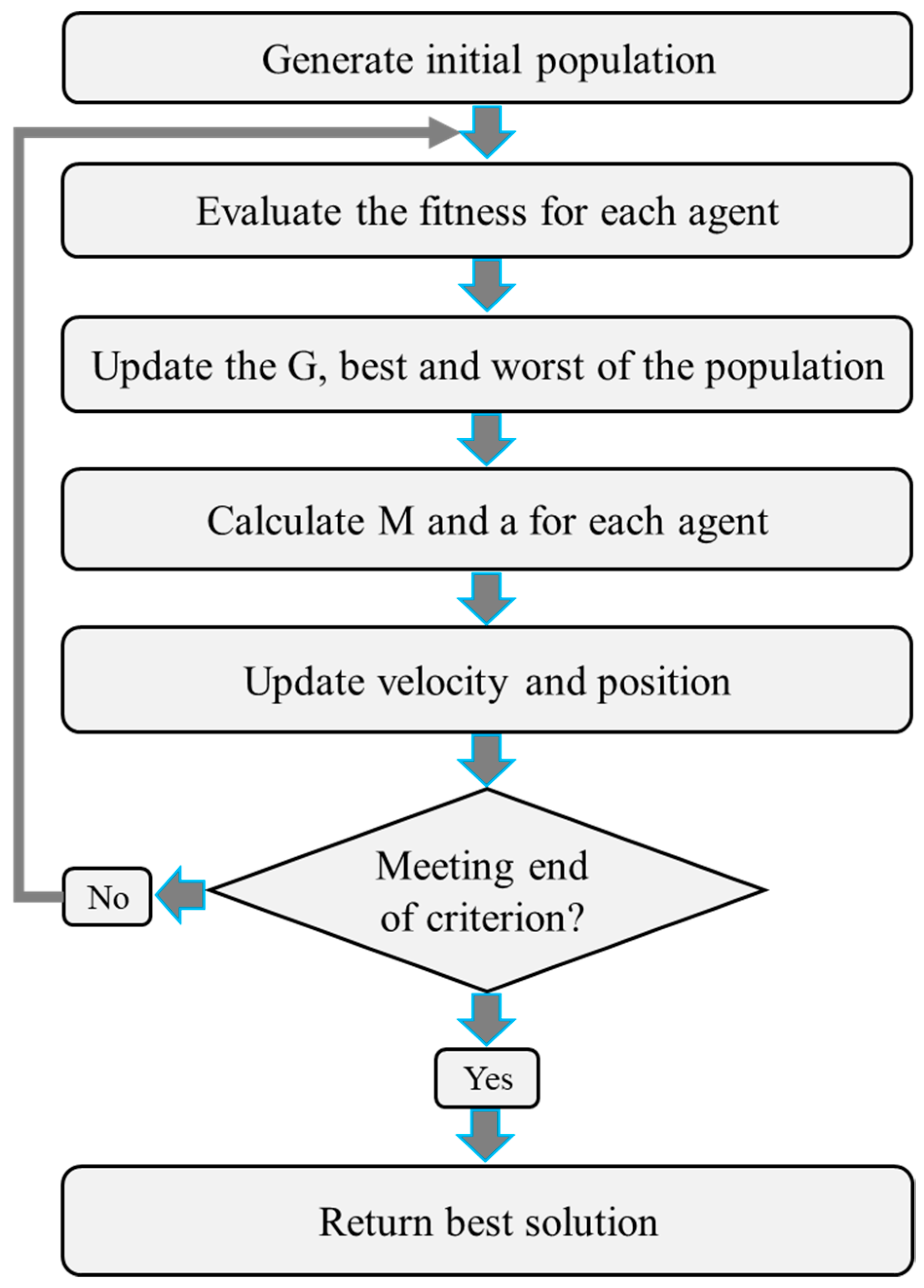
2.4.2. The Proposed Algorithm (IGSA)
2.4.3. The Objective Function (Fitness)
2.5. Comparison with Other Methods
3. Experimental Results
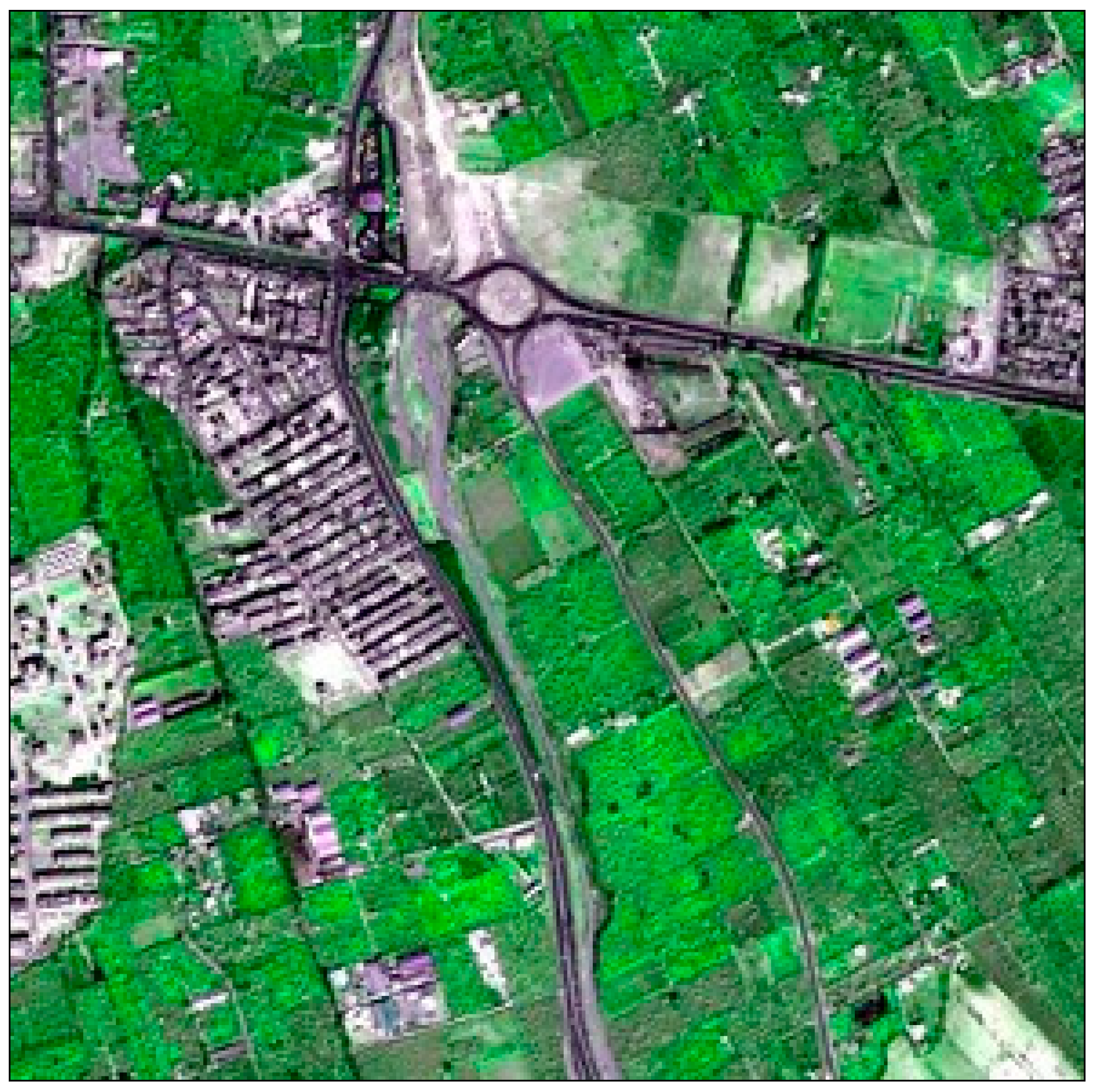
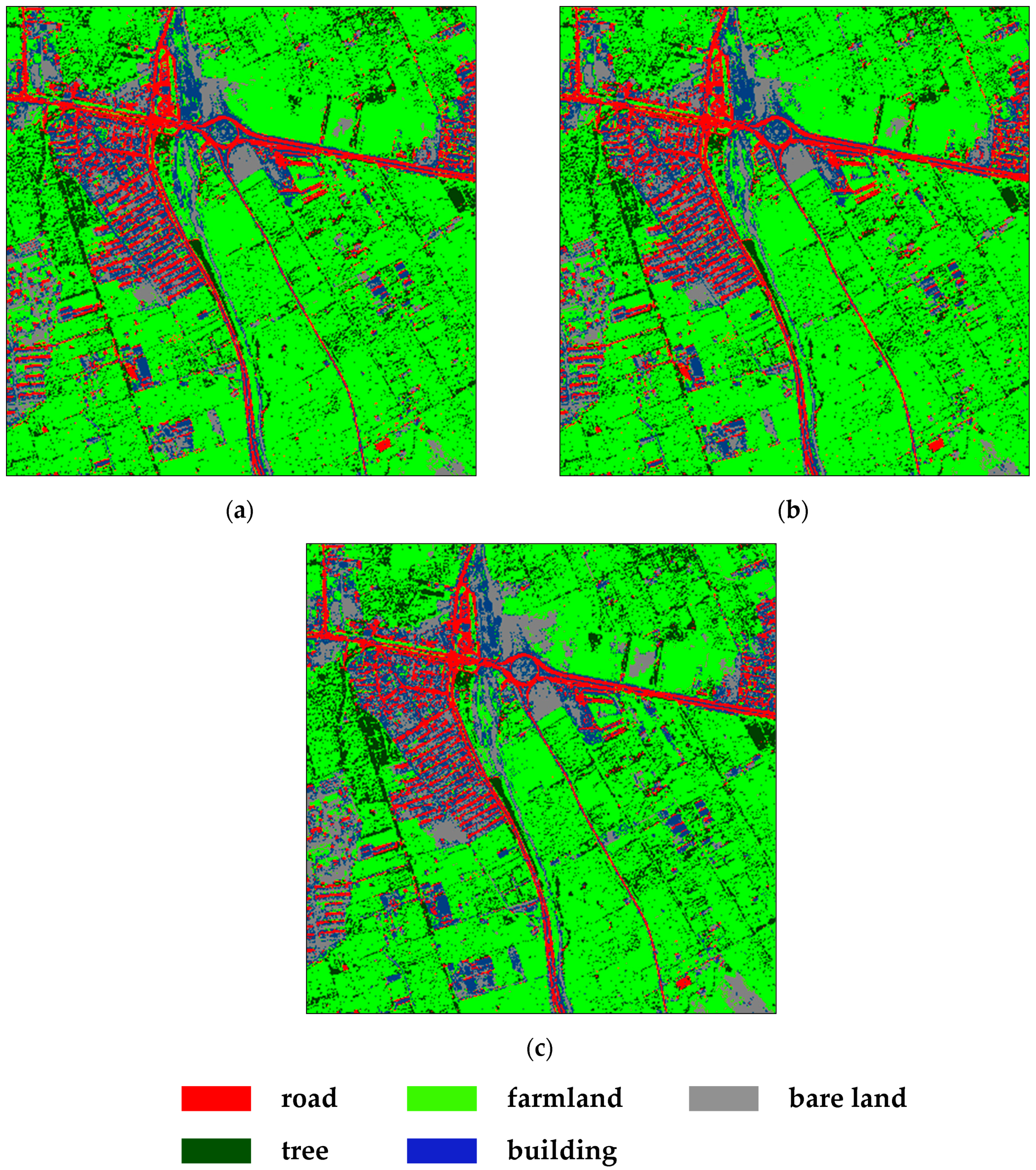
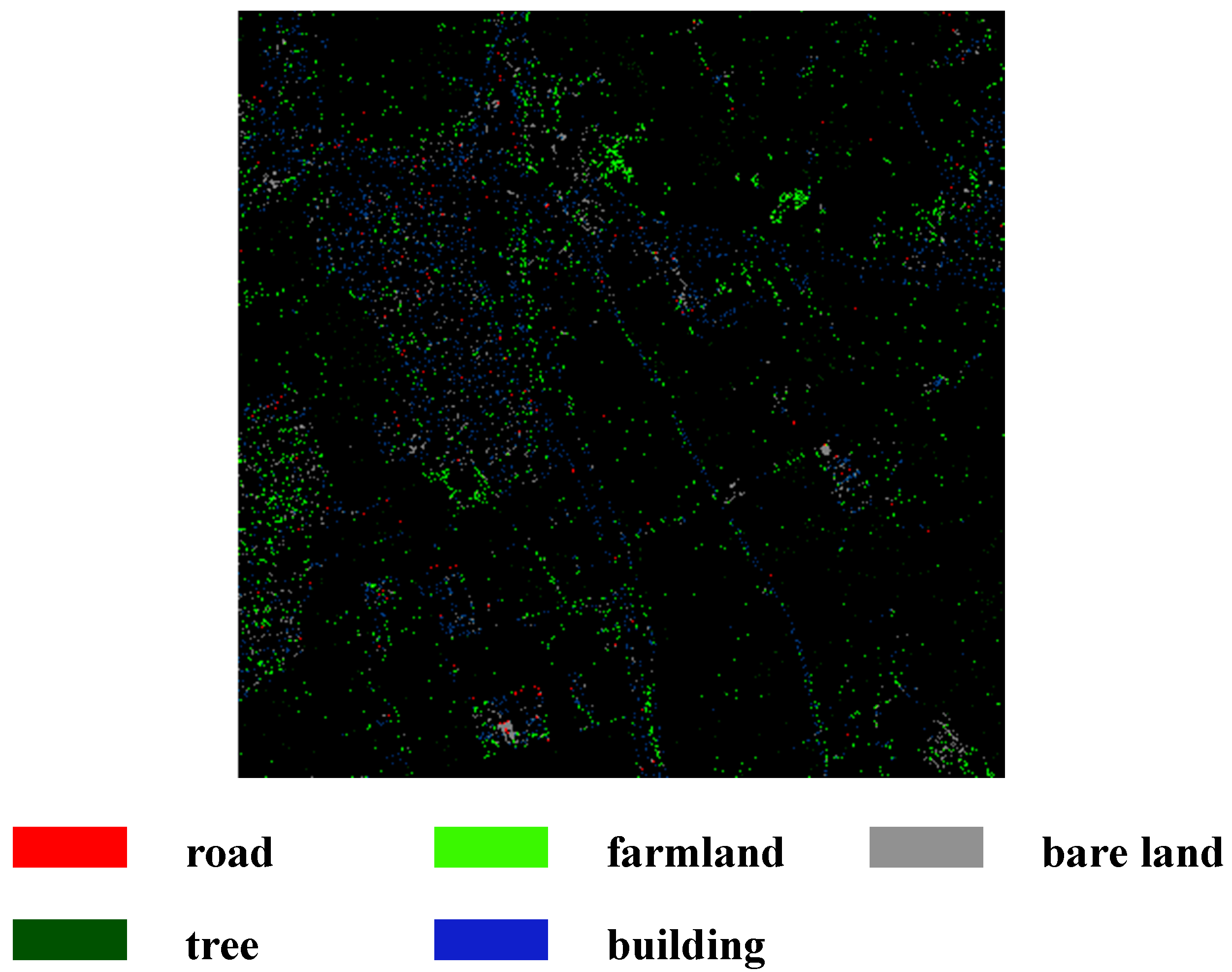
3.1. Multispectral Image
- The algorithm well preserved the road network.
- The different vegetation covers were separated from each other effectively.
- It distinguished between the two classes of bare land and building properly.
3.2. Hyperspectral Images
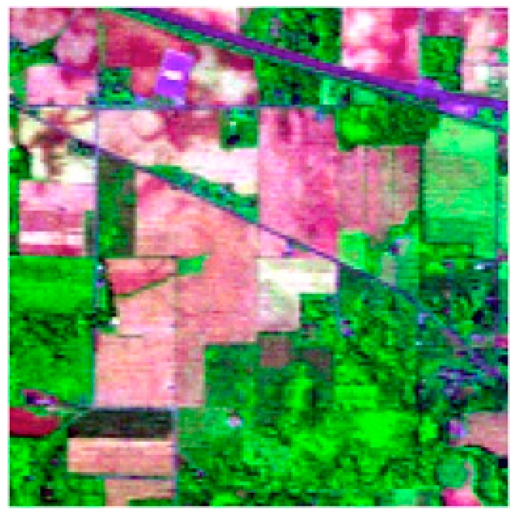
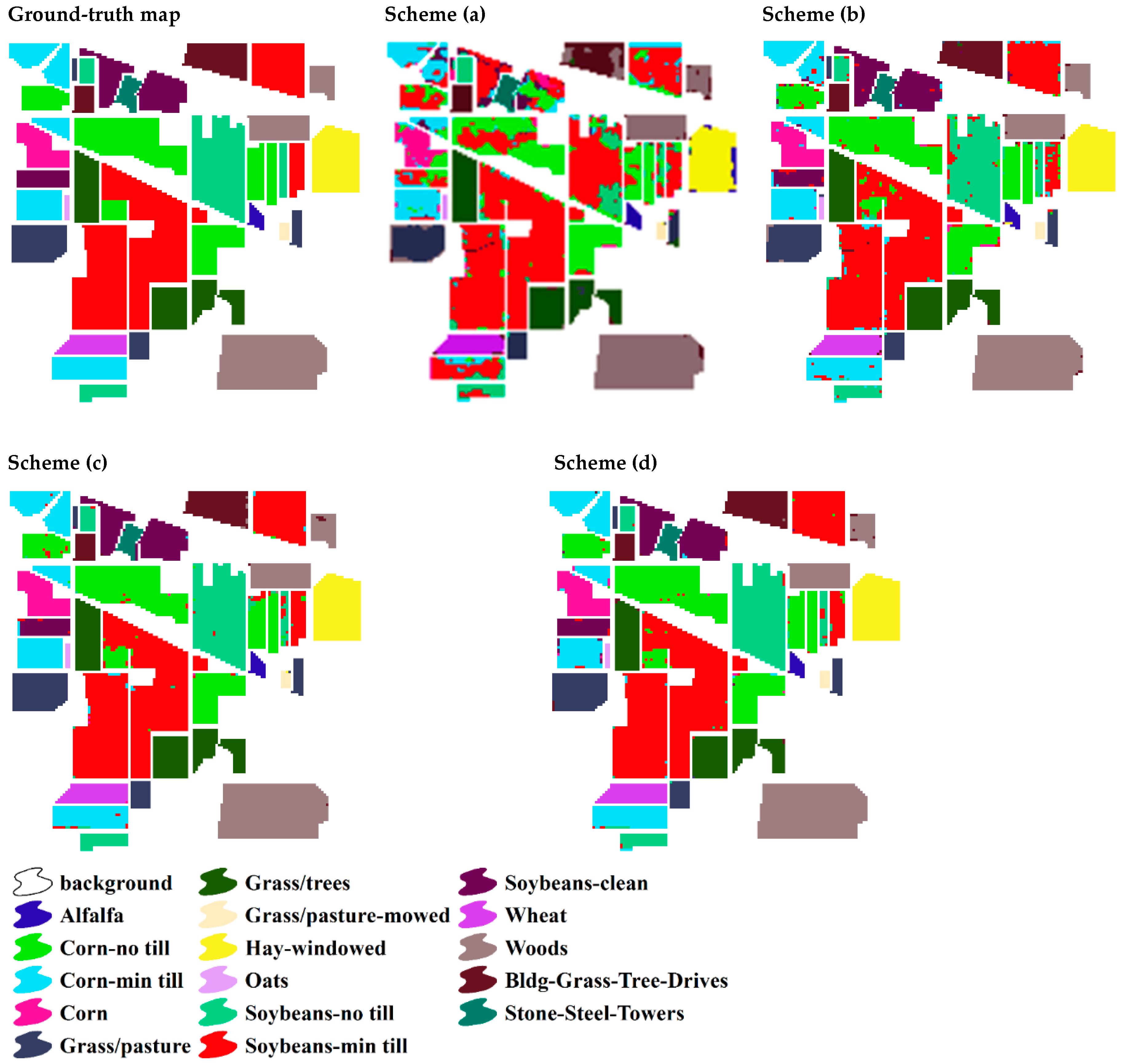
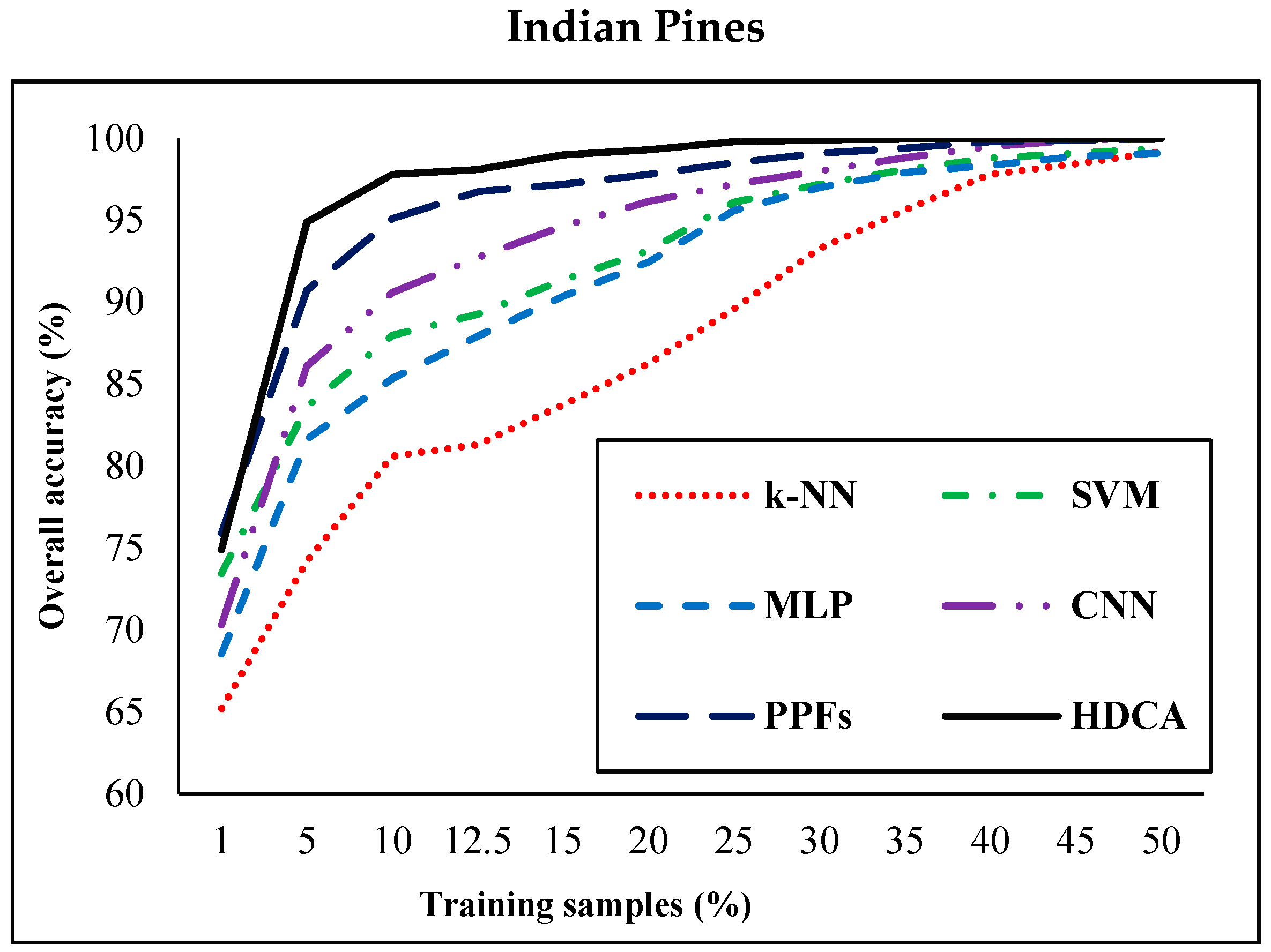
3.2.1. Indian Pines Dataset
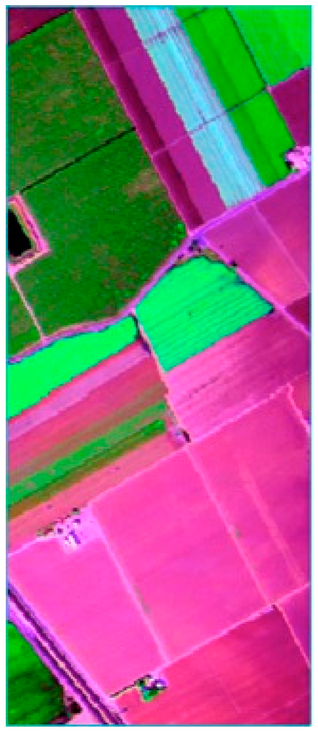
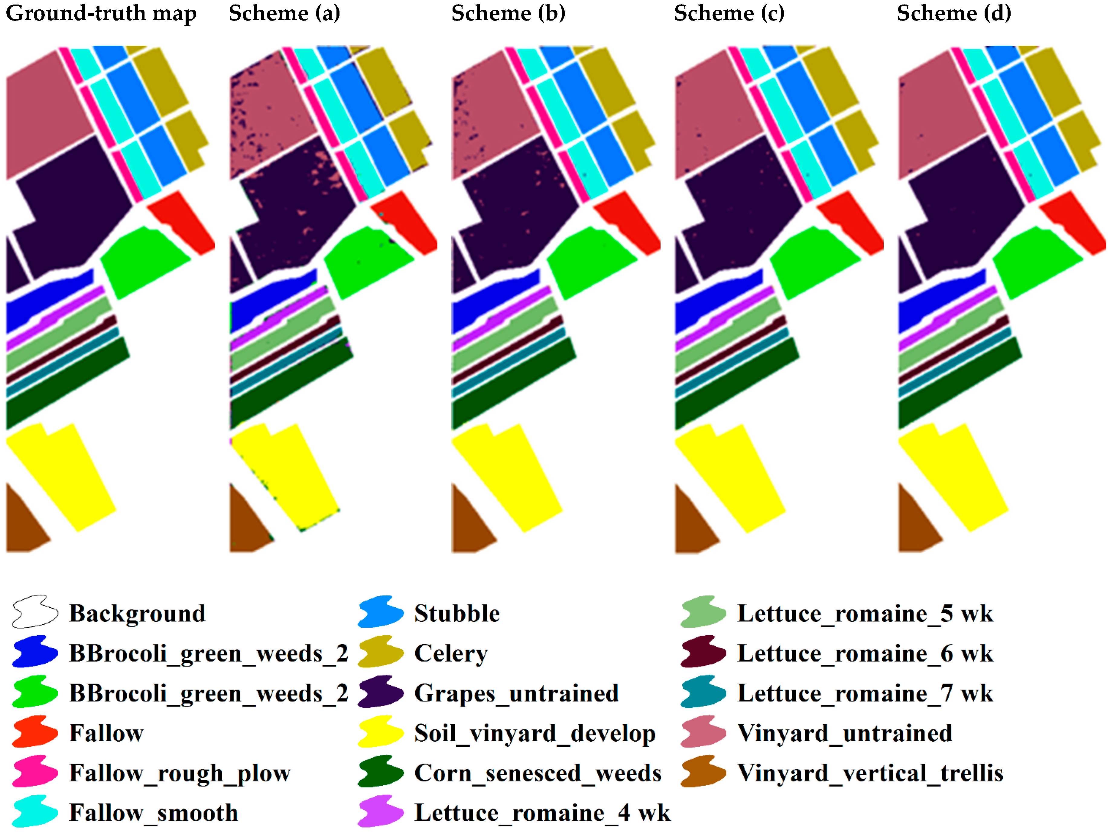
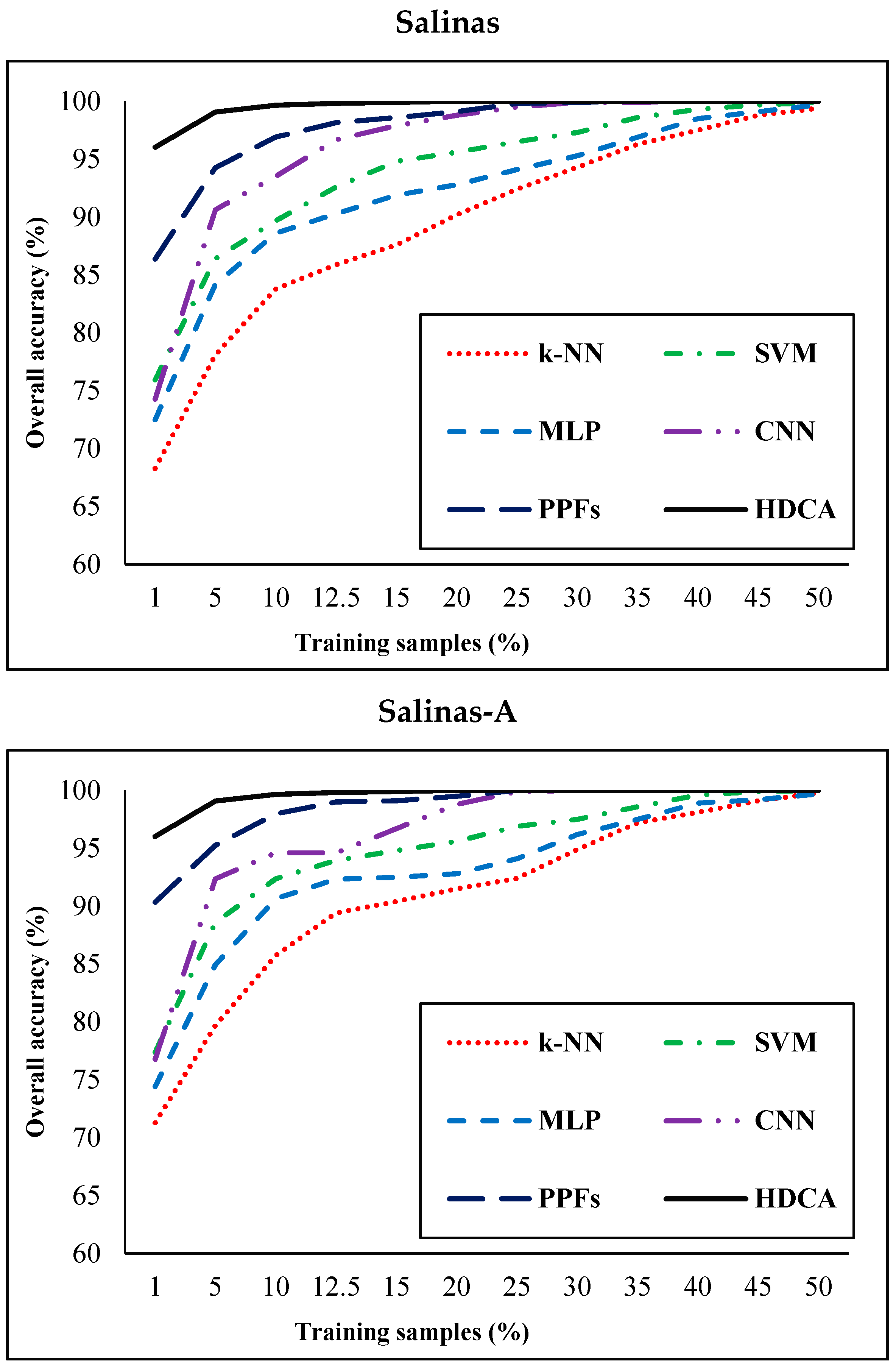
3.2.2. Salinas Dataset
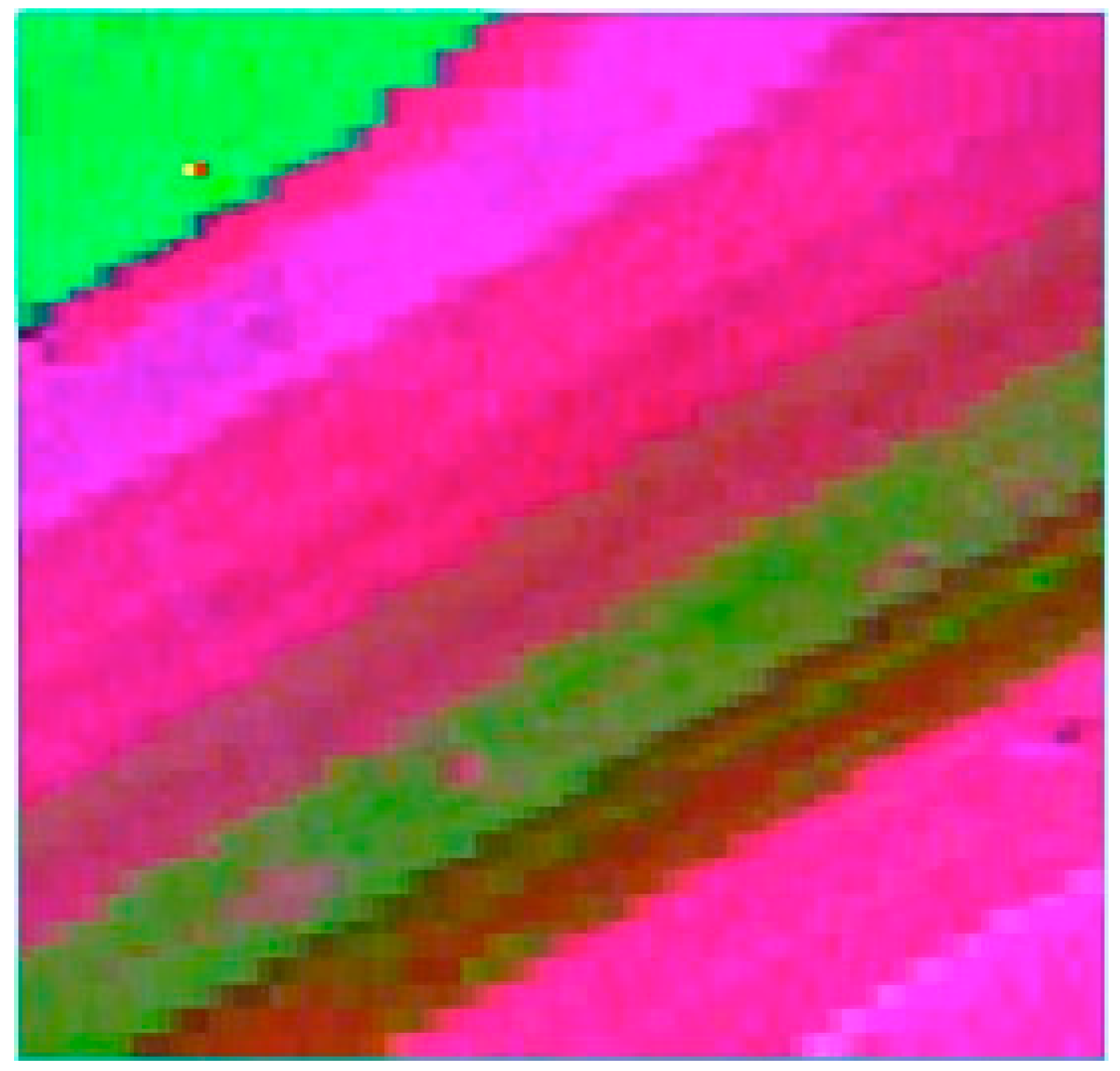
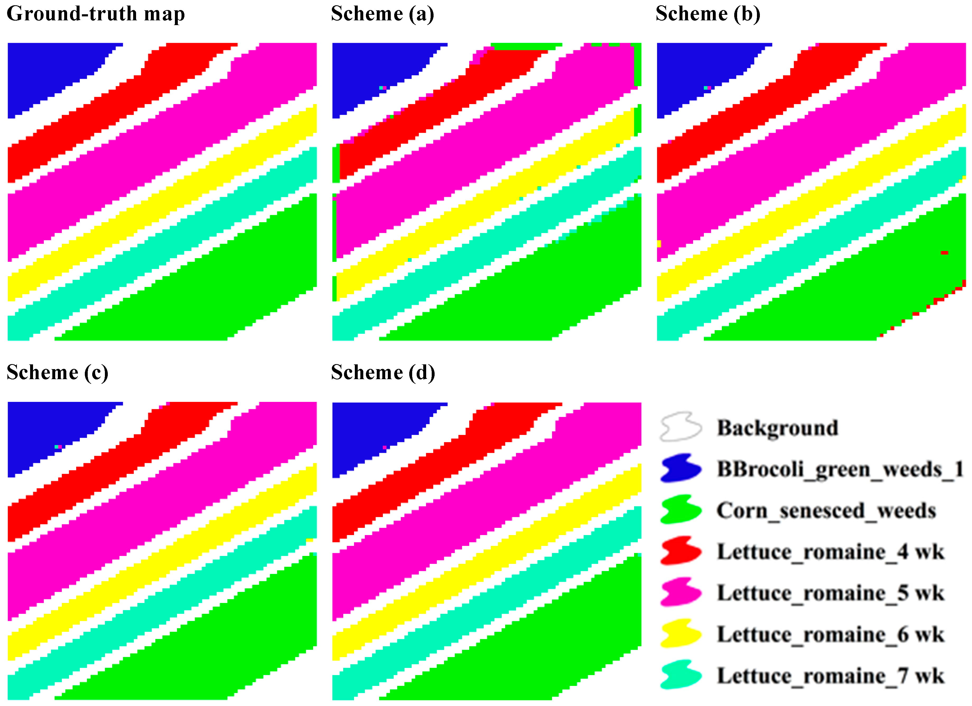
3.2.3. Salinas-A Scene Dataset
4. Discussion
5. Conclusions
Author Contributions
Funding
Acknowledgments
Conflicts of Interest
Appendix A


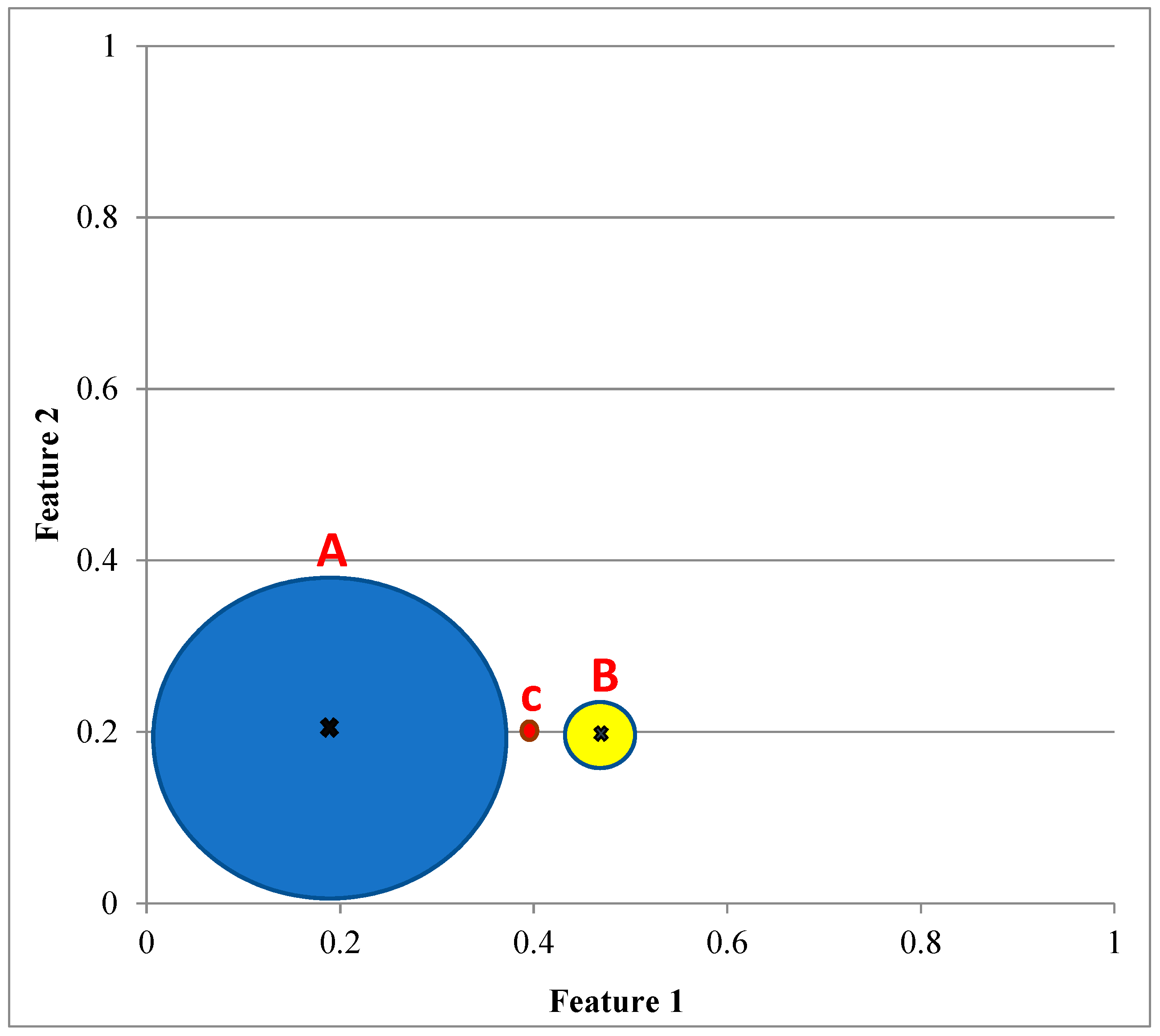
| Point | Feature 1_A | Feature 2_A | Feature 1_B | Feature 2_B |
|---|---|---|---|---|
| 1 | 0.1 | 0.05 | 0.491 | 0.206 |
| 2 | 0.12 | 0.05 | 0.502 | 0.216 |
| 3 | 0.15 | 0.22 | 0.521 | 0.196 |
| 4 | 0.2 | 0.15 | 0.484 | 0.184 |
| 5 | 0.25 | 0.06 | 0.493 | 0.202 |
| 6 | 0.23 | 0.37 | 0.509 | 0.209 |
| 7 | 0.26 | 0.15 | 0.501 | 0.201 |
| 8 | 0.3 | 0.06 | 0.507 | 0.207 |
| 9 | 0.35 | 0.14 | 0.509 | 0.204 |
| 10 | 0.38 | 0.13 | 0.508 | 0.189 |
| 11 | 0.25 | 0.29 | 0.511 | 0.203 |
| 12 | 0.06 | 0.2 | 0.502 | 0.202 |
| 13 | 0.05 | 0.23 | 0.513 | 0.215 |
| 14 | 0.18 | 0.16 | 0.514 | 0.186 |
| 15 | 0.2 | 0.33 | 0.515 | 0.208 |
| 16 | 0.13 | 0.35 | 0.516 | 0.206 |
| 17 | 0.16 | 0.3 | 0.507 | 0.195 |
| 18 | 0.19 | 0.36 | 0.499 | 0.201 |
| 19 | 0.31 | 0.1 | 0.485 | 0.218 |
| 20 | 0.32 | 0.14 | 0.487 | 0.187 |
| 21 | 0.35 | 0.13 | 0.486 | 0.196 |
| 22 | 0.26 | 0.21 | 0.489 | 0.191 |
| 23 | 0.32 | 0.24 | 0.485 | 0.185 |
| 24 | 0.29 | 0.21 | 0.488 | 0.218 |
| 25 | 0.26 | 0.27 | 0.505 | 0.192 |
| 26 | 0.08 | 0.38 | 0.489 | 0.209 |
| 27 | 0.05 | 0.21 | 0.491 | 0.191 |
| 28 | 0.04 | 0.02 | 0.486 | 0.186 |
| 29 | 0.03 | 0.2 | 0.5 | 0.211 |
| 30 | 0.14 | 0.3 | 0.513 | 0.193 |
| Statistical Parameters | Feature 1_A | Feature 2_A | Feature 1_B | Feature 2_B |
|---|---|---|---|---|
| Mean | 0.2 | 0.2 | 0.5 | 0.2 |
| SD | 0.1044 | 0.1038 | 0.0114 | 0.0103 |
- Euclidean distance
- WMD
References
- Schowengerdt, R.A. Techniques for Image Processing and Classifications in Remote Sensing; Academic Press: Cambridge, MA, USA, 2012. [Google Scholar]
- Bolstad, P.; Lillesand, T. Rapid maximum likelihood classification. Photogramm. Eng. Remote Sens. 1991, 57, 67–74. [Google Scholar]
- Bishop, C.; Bishop, C.M. Neural Networks for Pattern Recognition; Oxford University Press: Oxford, UK, 1995. [Google Scholar]
- Cortes, C.; Vapnik, V. Support-vector networks. Mach. Learn. 1995, 20, 273–297. [Google Scholar] [CrossRef] [Green Version]
- Freund, Y.; Mason, L. The alternating decision tree learning algorithm. In icml; Morgan Kaufmann Publishers Inc.: San Francisco, CA, USA, 1999; pp. 124–133. [Google Scholar]
- Bryll, R.; Gutierrez-Osuna, R.; Quek, F. Attribute bagging: Improving accuracy of classifier ensembles by using random feature subsets. Pattern Recognit. 2003, 36, 1291–1302. [Google Scholar] [CrossRef]
- Weinberger, K.Q.; Blitzer, J.; Saul, L.K. Distance metric learning for large margin nearest neighbor classification. In Advances in Neural Information Processing Systems; Neural Information Processing Systems Foundation, Inc.: Vancouver, BC, Canada, 2006; pp. 1473–1480. [Google Scholar]
- Manning, C.D.; Raghavan, P.; Schutze, H. Introduction to Information Retrieval; Cambridge University Press: Cambridge, UK, 2008; Chapter 20; pp. 405–416. [Google Scholar]
- Makantasis, K.; Doulamis, A.D.; Doulamis, N.D.; Nikitakis, A. Tensor-based classification models for hyperspectral data analysis. IEEE Trans. Geosci. Remote Sens. 2018, 1–15. [Google Scholar] [CrossRef]
- Kotsia, I.; Guo, W.; Patras, I. Higher rank support tensor machines for visual recognition. Pattern Recognit. 2012, 45, 4192–4203. [Google Scholar] [CrossRef]
- Rashedi, E.; Nezamabadi-Pour, H. A stochastic gravitational approach to feature based color image segmentation. Eng. Appl. Artif. Intell. 2013, 26, 1322–1332. [Google Scholar] [CrossRef]
- Neumann, J.; Schnörr, C.; Steidl, G. Combined svm-based feature selection and classification. Mach. Learn. 2005, 61, 129–150. [Google Scholar] [CrossRef]
- Xia, J. Multiple Classifier Systems for the Classification of Hyperspectral Data. Ph.D. Thesis, Université de Grenoble, Grenoble, France, 2014. [Google Scholar]
- Moghaddam, M.H.R.; Sedighi, A.; Fasihi, S.; Firozjaei, M.K. Effect of environmental policies in combating aeolian desertification over sejzy plain of iran. Aeolian Res. 2018, 35, 19–28. [Google Scholar] [CrossRef]
- Hatamlou, A.; Abdullah, S.; Nezamabadi-Pour, H. A combined approach for clustering based on k-means and gravitational search algorithms. Swarm Evol. Comput. 2012, 6, 47–52. [Google Scholar] [CrossRef]
- Rezaei, M.; Nezamabadi-Pour, H. Using gravitational search algorithm in prototype generation for nearest neighbor classification. Neurocomputing 2015, 157, 256–263. [Google Scholar] [CrossRef]
- Li, S.; Wu, H.; Wan, D.; Zhu, J. An effective feature selection method for hyperspectral image classification based on genetic algorithm and support vector machine. Knowl.-Based Syst. 2011, 24, 40–48. [Google Scholar] [CrossRef]
- Shelokar, P.; Jayaraman, V.K.; Kulkarni, B.D. An ant colony approach for clustering. Anal. Chim. Acta 2004, 509, 187–195. [Google Scholar] [CrossRef]
- Krishna, K.; Murty, M.N. Genetic k-means algorithm. IEEE Trans. Syst. Man Cybern. Part B (Cybern.) 1999, 29, 433–439. [Google Scholar] [CrossRef] [PubMed]
- Qinand, A.; Suganthan, P.N. Kernel neural gas algorithms with application to cluster analysis. In Proceedings of the 17th International Conference on Pattern Recognition, Cambridge, UK, 23–26 August 2004; pp. 617–620. [Google Scholar]
- Omran, M.G.; Engelbrecht, A.P.; Salman, A. Image classification using particle swarm optimization. In Recent Advances in Simulated Evolution and Learning; World Scientific: Singapore, 2004; pp. 347–365. [Google Scholar]
- Luo, Y.; Zou, J.; Yao, C.; Zhao, X.; Li, T.; Bai, G. Hsi-cnn: A novel convolution neural network for hyperspectral image. In Proceedings of the 2018 International Conference on Audio, Language and Image Processing (ICALIP), Prague, Czech Republic, 9–10 July 2018; pp. 464–469. [Google Scholar]
- Gao, Q.; Lim, S.; Jia, X. Hyperspectral image classification using convolutional neural networks and multiple feature learning. Remote Sens. 2018, 10, 299. [Google Scholar] [CrossRef]
- Chen, Y.; Jiang, H.; Li, C.; Jia, X.; Ghamisi, P. Deep feature extraction and classification of hyperspectral images based on convolutional neural networks. IEEE Trans. Geosci. Remote Sens. 2016, 54, 6232–6251. [Google Scholar] [CrossRef]
- Zhao, W.; Du, S. Spectral–spatial feature extraction for hyperspectral image classification: A dimension reduction and deep learning approach. IEEE Trans. Geosci. Remote Sens. 2016, 54, 4544–4554. [Google Scholar] [CrossRef]
- Yue, J.; Zhao, W.; Mao, S.; Liu, H. Spectral–spatial classification of hyperspectral images using deep convolutional neural networks. Remote Sens. Lett. 2015, 6, 468–477. [Google Scholar] [CrossRef]
- Aptoula, E.; Ozdemir, M.C.; Yanikoglu, B. Deep learning with attribute profiles for hyperspectral image classification. IEEE Geosci. Remote Sens. 2016, 13, 1970–1974. [Google Scholar] [CrossRef]
- Zhao, W.; Guo, Z.; Yue, J.; Zhang, X.; Luo, L. On combining multiscale deep learning features for the classification of hyperspectral remote sensing imagery. Int. J. Remote Sens 2015, 36, 3368–3379. [Google Scholar] [CrossRef]
- Schutz, B. Gravity from the Ground Up: An Introductory Guide to Gravity and General Relativity; Cambridge University Press: Cambridge, UK, 2003. [Google Scholar]
- Halliday, D.; Resnick, R.; Walker, J. Fundamentals of Physics; Wiley and Sons: New York, NY, USA, 1993. [Google Scholar]
- Wright, W.E. Gravitational clustering. Pattern Recognit. 1977, 9, 151–166. [Google Scholar] [CrossRef]
- Lai, A.H.; Yung, H. Segmentation of color images based on the gravitational clustering concept. Opt. Eng. 1998, 37, 989–1001. [Google Scholar]
- Kundu, S. Gravitational clustering: A new approach based on the spatial distribution of the points. Pattern Recognit. 1999, 32, 1149–1160. [Google Scholar] [CrossRef]
- Chen, C.-Y.; Hwang, S.-C.; Oyang, Y.-J. A statistics-based approach to control the quality of subclusters in incremental gravitational clustering. Pattern Recognit. 2005, 38, 2256–2269. [Google Scholar] [CrossRef]
- Long, T.; Jin, L.-W. A new simplified gravitational clustering method for multi-prototype learning based on minimum classification error training. In Advances in Machine Vision, Image Processing, and Pattern Analysis; Springer: Berlin, Germany, 2006; pp. 168–175. [Google Scholar]
- Han, X.; Quan, L.; Xiong, X.; Almeter, M.; Xiang, J.; Lan, Y. A novel data clustering algorithm based on modified gravitational search algorithm. Eng. Appl. Artif. Intell. 2017, 61, 1–7. [Google Scholar] [CrossRef]
- Rashedi, E.; Nezamabadi-Pour, H.; Saryazdi, S. Gsa: A gravitational search algorithm. Inf. Sci. 2009, 179, 2232–2248. [Google Scholar] [CrossRef]
- Dowlatshahi, M.B.; Nezamabadi-pour, H. Ggsa: A grouping gravitational search algorithm for data clustering. Eng. Appl. Artif. Intell. 2014, 36, 114–121. [Google Scholar] [CrossRef]
- Waske, B.; van der Linden, S.; Benediktsson, J.A.; Rabe, A.; Hostert, P. Sensitivity of support vector machines to random feature selection in classification of hyperspectral data. IEEE Trans. Geosci. Remote Sens. 2010, 48, 2880–2889. [Google Scholar] [CrossRef]
- Hu, W.; Huang, Y.; Wei, L.; Zhang, F.; Li, H. Deep convolutional neural networks for hyperspectral image classification. J. Sens. 2015, 2015. [Google Scholar] [CrossRef]
- Li, W.; Wu, G.; Zhang, F.; Du, Q. Hyperspectral image classification using deep pixel-pair features. IEEE Trans. Geosci. Remote Sens. 2017, 55, 844–853. [Google Scholar] [CrossRef]
- Song, B.; Li, J.; Dalla Mura, M.; Li, P.; Plaza, A.; Bioucas-Dias, J.M.; Benediktsson, J.A.; Chanussot, J. Remotely sensed image classification using sparse representations of morphological attribute profiles. IEEE Trans. Geosci. Remote Sens. 2014, 52, 5122–5136. [Google Scholar] [CrossRef]
- Shahdoosti, H.R.; Mirzapour, F. Spectral–spatial feature extraction using orthogonal linear discriminant analysis for classification of hyperspectral data. Eur. J. Remote Sens. 2017, 50, 111–124. [Google Scholar] [CrossRef] [Green Version]
- Haridas, N.; Sowmya, V.; Soman, K. Comparative analysis of scattering and random features in hyperspectral image classification. Procedia Comput. Sci. 2015, 58, 307–314. [Google Scholar] [CrossRef]
- Xu, Y.; Wu, Z.; Wei, Z. Spectral–spatial classification of hyperspectral image based on low-rank decomposition. IEEE J. Sel. Top. Appl. Earth Obs. Remote Sens. 2015, 8, 2370–2380. [Google Scholar] [CrossRef]
- Su, H.; Yong, B.; Du, P.; Liu, H.; Chen, C.; Liu, K. Dynamic classifier selection using spectral-spatial information for hyperspectral image classification. J. Appl. Remote Sens. 2014, 8, 085095. [Google Scholar] [CrossRef]
- Ran, L.; Zhang, Y.; Wei, W.; Zhang, Q. A hyperspectral image classification framework with spatial pixel pair features. Sensors 2017, 17, 2421. [Google Scholar] [CrossRef] [PubMed]
- Iliopoulos, A.-S.; Liu, T.; Sun, X. Hyperspectral image classification and clutter detection via multiple structural embeddings and dimension reductions. arXiv, 2015; arXiv:1506.01115. [Google Scholar]
- Dópido, I.; Zortea, M.; Villa, A.; Plaza, A.; Gamba, P. Unmixing prior to supervised classification of remotely sensed hyperspectral images. IEEE Geosci. Remote Sens. Lett. 2011, 8, 760–764. [Google Scholar] [CrossRef]
- Bernabé, S.; Marpu, P.R.; Plaza, A.; Dalla Mura, M.; Benediktsson, J.A. Spectral–spatial classification of multispectral images using kernel feature space representation. IEEE Geosci. Remote Sens. Lett. 2014, 11, 288–292. [Google Scholar] [CrossRef]
- Camps-Valls, G.; Gomez-Chova, L.; Muñoz-Marí, J.; Vila-Francés, J.; Calpe-Maravilla, J. Composite kernels for hyperspectral image classification. IEEE Geosci. Remote Sens. Lett. 2006, 3, 93–97. [Google Scholar] [CrossRef]
- Ramzi, P.; Samadzadegan, F.; Reinartz, P. Classification of hyperspectral data using an adaboostsvm technique applied on band clusters. IEEE J. Sel. Top. Appl. Earth Obs. Remote Sens. 2014, 7, 2066–2079. [Google Scholar] [CrossRef]
- Thanh Noi, P.; Kappas, M. Comparison of random forest, k-nearest neighbor, and support vector machine classifiers for land cover classification using sentinel-2 imagery. Sensors 2018, 18, 18. [Google Scholar] [CrossRef] [PubMed]
- Firozjaei, M.K.; Kiavarz, M.; Nematollahi, O.; Karimpour Reihan, M.; Alavipanah, S.K. An evaluation of energy balance parameters, and the relations between topographical and biophysical characteristics using the mountainous surface energy balance algorithm for land (sebal). Int. J. Remote Sens. 2019, 1–31. [Google Scholar] [CrossRef]
- Firozjaei, M.K.; Kiavarz, M.; Alavipanah, S.K.; Lakes, T.; Qureshi, S. Monitoring and forecasting heat island intensity through multi-temporal image analysis and cellular automata-markov chain modelling: A case of babol city, iran. Ecol. Indic. 2018, 91, 155–170. [Google Scholar] [CrossRef]
- Panah, S.; Mogaddam, M.K.; Firozjaei, M.K. Monitoring spatiotemporal changes of heat island in babol city due to land use changes. Int. Arch. Photogramm. Remote Sens. Spat. Inf. Sci. 2017, 42. [Google Scholar]
- Weng, Q.; Firozjaei, M.K.; Sedighi, A.; Kiavarz, M.; Alavipanah, S.K. Statistical analysis of surface urban heat island intensity variations: A case study of Babol city, Iran. GISci. Remote Sens. 2019, 56, 576–604. [Google Scholar] [CrossRef]
- Heumann, B.W. An object-based classification of mangroves using a hybrid decision tree—Support vector machine approach. Remote Sens. 2011, 3, 2440–2460. [Google Scholar] [CrossRef]
- Qian, Y.; Zhou, W.; Yan, J.; Li, W.; Han, L. Comparing machine learning classifiers for object-based land cover classification using very high resolution imagery. Remote Sens. 2015, 7, 153–168. [Google Scholar] [CrossRef]
- Karimi Firozjaei, M.; Kiavarz Mogaddam, M.; Alavi Panah, S.K. Monitoring and predicting spatial-temporal changes heat island in babol city due to urban sprawl and land use changes. J. Geospat. Inf. Technol. 2017, 5, 123–151. [Google Scholar] [CrossRef]
- Karimi Firuzjaei, M.; Kiavarz Moghadam, M.; Mijani, N.; Alavi Panah, S.K. Quantifying the degree-of-freedom, degree-of-sprawl and degree-of-goodness of urban growth tehran and factors affecting it using remote sensing and statistical analyzes. J. Geomat. Sci. Technol. 2018, 7, 89–107. [Google Scholar]
- Haralick, R.M.; Shanmugam, K. Textural features for image classification. IEEE Trans. Syst. Man Cybern. 1973, 610–621. [Google Scholar] [CrossRef]
- Plaza, A.; Martinez, P.; Plaza, J.; Perez, R. Dimensionality reduction and classification of hyperspectral image data using sequences of extended morphological transformations. IEEE Trans. Geosci Remote Sens. 2005, 43, 466–479. [Google Scholar] [CrossRef] [Green Version]
- Haridas, N.; Sowmya, V.; Soman, K. Hyperspectral image classification using random kitchen sink and regularized least squares. In Proceedings of the 2015 International Conference on Communications and Signal Processing (ICCSP), Melmaruvathur, India, 2–4 April 2015; pp. 1665–1669. [Google Scholar]
- Santara, A.; Mani, K.; Hatwar, P.; Singh, A.; Garg, A.; Padia, K.; Mitra, P. Bass net: Band-adaptive spectral-spatial feature learning neural network for hyperspectral image classification. IEEE Trans. Geosci Remote Sens. 2017, 55, 5293–5301. [Google Scholar] [CrossRef]


| HDCA | User’s Accuracy | Producer’s Accuracy | ||||||||
| Road | tree | farmland | building | Bare land | road | tree | farmland | building | bare land | |
| Road | 98.56% | 0% | 0% | 1.44% | 0% | 90.51% | 0% | 0% | 1.69% | 0% |
| Tree | 0.56% | 99.22% | 0.22% | 0% | 0% | 0.51 | 99.00% | 0.10% | 0% | 0% |
| farmland | 0% | 0.45% | 99.55% | 0% | 0% | 0% | 1.00% | 99.65% | 0% | 0% |
| building | 9.78% | 0% | 0.44% | 80.67% | 9.11% | 8.98% | 0% | 0.20% | 94.53% | 10.90 |
| bare land | 0% | 0% | 0.14% | 4.14% | 95.71% | 0% | 0% | 0.05% | 3.78% | 89.10% |
| Overall Accuracy: 95.69% | Cohen’s Kappa Coefficient: 94.35% | |||||||||
| SVM | User’s Accuracy | Producer’s Accuracy | ||||||||
| Road | tree | farmland | building | Bare land | Road | tree | farmland | building | bare land | |
| Road | 98.67% | 0% | 0.11% | 1.22% | 0% | 88.62% | 0% | 0.04% | 1.52% | 0% |
| Tree | 0.89% | 98.56% | 0.56% | 0% | 0% | 0.80% | 98.78% | 0.25% | 0% | 0% |
| farmland | 0% | 0.50% | 99.50% | 0% | 0% | 0% | 1.11% | 99.25% | 0% | 0% |
| building | 11.78% | 0% | 0.89% | 76.78% | 10.33% | 10.58% | 0% | 0.40% | 95.18% | 12.13% |
| bare land | 0% | 0.14% | 0.14% | 3.43% | 96.29% | 0% | 0.11% | 0.04% | 3.31% | 87.87% |
| Overall Accuracy: 95.00% | Cohen’s Kappa Coefficient: 93.95% | |||||||||
| MLC | User’s Accuracy | Producer’s Accuracy | ||||||||
| Road | tree | farmland | building | Bare land | road | tree | farmland | building | bare land | |
| Road | 97.89% | 0.33% | 0.11% | 1.67% | 0% | 90.45% | 0.32% | 0.05% | 2.07% | 0% |
| Tree | 0.44% | 99.33% | 0.22% | 0% | 0% | 0.41% | 93.91% | 0.10% | 0% | 0% |
| farmland | 0% | 2.70% | 95.55% | 0.60% | 1.15% | 0% | 5.67% | 99.32% | 1.66% | 2.78% |
| building | 9.89% | 0% | 1.11% | 74.56% | 14.44% | 9.14% | 0% | 0.52% | 92.68% | 15.74% |
| bare land | 0% | 0.14% | 0% | 3.71% | 96.14% | 0% | 0.11% | 0% | 3.59% | 81.48% |
| Overall Accuracy: 93.15% | Cohen’s Kappa Coefficient: 91.06% | |||||||||
| No | Class | Pixels | No | Class | Pixels |
|---|---|---|---|---|---|
| 1 | Alfalfa | 46 | 9 | Hay-windowed | 478 |
| 2 | Bldg-Grass-Tree-Drives | 386 | 10 | Oats | 20 |
| 3 | Corn-no till | 1428 | 11 | Soybeans-no till | 972 |
| 4 | Corn-min till | 830 | 12 | Soybeans-min till | 2455 |
| 5 | Corn | 237 | 13 | Soybeans-clean | 593 |
| 6 | Grass/pasture | 483 | 14 | Stone-Steel-Towers | 93 |
| 7 | Grass/trees | 730 | 15 | Wheat | 205 |
| 8 | Grass/pasture-mowed | 28 | 16 | Woods | 1265 |
| Class | UA | PA | Class | UA | PA |
|---|---|---|---|---|---|
| Alfalfa | 100 | 100 | Oats | 100 | 100 |
| Corn-no till | 97.92 | 95.25 | Soybeans-no till | 97.03 | 96.81 |
| Corn-min till | 96.67 | 97.05 | Soybeans-min till | 96.22 | 98.05 |
| Corn | 97.71 | 100 | Soybeans-clean | 98.3 | 97.38 |
| Grass/pasture | 99.77 | 99.77 | Wheat | 100 | 99.46 |
| Grass/trees | 100 | 100 | Woods | 99.30 | 99.30 |
| Grass/pasture-mowed | 100 | 92.00 | Bldg-Grass-Tree | 97.42 | 97.98 |
| Hay-windowed | 99.77 | 100 | Stone-Steel-Towers | 100 | 90.48 |
| Scheme. | (a) 1% | (b) 5% | (c) 10% | (d) 12.5% | |
| Overall Accuracy | 74.89 | 94.94 | 97.88 | 98.09 | |
| Cohen’s Kappa | 0.7075 | 0.9423 | 0.9759 | 0.9789 | |
| No | Class | Pixels | No | Class | Pixels |
|---|---|---|---|---|---|
| 1 | BBrocoli_green_weeds_1 | 2009 | 9 | Soil_vinyard_develop | 6203 |
| 2 | BBrocoli_green_weeds_2 | 3726 | 10 | Corn_senesced_weeds | 3278 |
| 3 | Fallow | 1976 | 11 | Lettuce_romaine_4 wk | 1068 |
| 4 | Fallow_rough_plow | 1394 | 12 | Lettuce_romaine_5 wk | 1927 |
| 5 | Fallow_smooth | 2678 | 13 | Lettuce_romaine_6 wk | 916 |
| 6 | Stubble | 3959 | 14 | Lettuce_romaine_7 wk | 1070 |
| 7 | Celery | 3579 | 15 | Vinyard_untrained | 7268 |
| 8 | Grapes_untrained | 11271 | 16 | Vinyard_vertical_trellis | 1807 |
| Class | UA | PA | Class | UA | PA |
|---|---|---|---|---|---|
| BBrocoli_green_weeds_1 | 100 | 100 | Soil_vinyard_develop | 99.86 | 99.98 |
| BBrocoli_green_weeds_2 | 100 | 100 | Corn_senesced_weeds | 99.66 | 99.76 |
| Fallow | 100 | 100 | Lettuce_romaine_4 wk | 100 | 98.86 |
| Fallow_rough_plow | 99.52 | 99.76 | Lettuce_romaine_5 wk | 99.88 | 99.83 |
| Fallow_smooth | 100 | 99.71 | Lettuce_romaine_6 wk | 100 | 100 |
| Stubble | 100 | 99.76 | Lettuce_romaine_7 wk | 100 | 100 |
| Celery | 100 | 99.88 | Vinyard_untrained | 98.89 | 99.26 |
| Grapes_untrained | 99.43 | 99.30 | Vinyard_vertical_trellis | 99.82 | 100 |
| Scheme | (a) 1% | (b) 5% | (c) 10% | (d) 12.5% | |
| Overall Accuracy | 96.03 | 99.08 | 97.66 | 99.82 | |
| Cohen’s Kappa | 0.9562 | 0.9903 | 0.9966 | 0.9983 | |
| No | Category | Pixels |
|---|---|---|
| 1 | BBrocoli_green_weeds_1 | 391 |
| 2 | Corn_senesced_weeds | 1343 |
| 3 | Lettuce_romaine_4 wk | 616 |
| 4 | Lettuce_romaine_5 wk | 1525 |
| 5 | Lettuce_romaine_6 wk | 674 |
| 6 | Lettuce_romaine_7 wk | 799 |
| Class | UA | PA | ||
|---|---|---|---|---|
| BBrocoli_green_weeds_1 | 100 | 99.41 | ||
| Corn_senesced_weeds | 100 | 99.91 | ||
| Lettuce_romaine_4 wk | 100 | 99.63 | ||
| Lettuce_romaine_5 wk | 99.78 | 100 | ||
| Lettuce_romaine_6 wk | 99.66 | 100 | ||
| Lettuce_romaine_7 wk | 99.71 | 99.71 | ||
| Scheme | (a) 1% | (b) 5% | (c) 10% | (d) 12.5% |
| Overall accuracy | 96.22 | 99.46 | 99.85 | 99.91 |
| Cohen’s Kappa | 0.9526 | 0.9933 | 0.9981 | 0.9989 |
| Dataset | Training Samples (%) | k-NN | SVM | MLP | CNN | PPFs | Proposed (HDCA) |
|---|---|---|---|---|---|---|---|
| Indian Pines | 1 | 65.2 | 73.44 | 68.53 | 70.3 | 75.89 | 74.90 |
| 5 | 74.2 | 83.63 | 81.64 | 86.12 | 90.72 | 94.90 | |
| 10 | 80.6 | 87.97 | 85.35 | 90.6 | 95.11 | 97.81 | |
| 12.5 | 81.3 | 89.27 | 87.93 | 92.75 | 96.75 | 98.09 | |
| Salinas | 1 | 68.3 | 75.94 | 72.57 | 74.28 | 86.37 | 96.03 |
| 5 | 78.1 | 86.41 | 84.26 | 90.63 | 94.26 | 99.08 | |
| 10 | 83.8 | 89.68 | 88.61 | 93.52 | 96.91 | 99.66 | |
| 12.5 | 85.9 | 92.6 | 90.3 | 96.68 | 98.15 | 99.82 | |
| Salinas-A | 1 | 71.83 | 77.37 | 74.42 | 76.78 | 90.34 | 96.03 |
| 5 | 79.69 | 88.59 | 84.94 | 92.36 | 95.26 | 99.08 | |
| 10 | 85.75 | 92.36 | 90.65 | 94.61 | 97.97 | 99.66 | |
| 12.5 | 89.43 | 93.96 | 92.33 | 97.93 | 99.01 | 99.82 |
| Dataset | Training samples (%) | RKS-RLS a | SUnSALEMAP b | SVM-CK c | GURLS d | OLDA e | BASS Net f | CNN-MFL g | HIS-CNN h | Proposed (HDCA) |
|---|---|---|---|---|---|---|---|---|---|---|
| Indian Pines | 1 | - | - | 73.7 | - | 73.3 | - | - | - | 74.90 |
| 5 | - | 95 | 91.4 | 94.5 | - | - | - | 94.90 | ||
| 10 | 93.79 | 96.8 | 94.9 | 89.59 | 97.6 | 96.77 | 97.54 | - | 97.81 | |
| 12.5 | - | - | 95.8 | - | 97.8 | - | - | 99.09 | 98.09 | |
| Salinas | 1 | - | - | 95.6 | - | 96 | - | - | - | 96.03 |
| 5 | - | - | 98.7 | - | 99.4 | - | - | - | 99.08 | |
| 10 | - | - | 98.9 | - | 99.9 | 95.33 | 98.34 | - | 99.66 | |
| 12.5 | - | - | 99.1 | - | 99.9 | - | - | 98.95 | 99.82 | |
| Salinas-A | 1 | - | - | - | - | - | - | - | - | 96.03 |
| 5 | - | - | - | - | - | - | - | - | 99.08 | |
| 10 | 98.58 | - | - | 98.31 | - | - | - | - | 99.66 | |
| 12.5 | - | - | - | - | - | - | - | - | 99.82 |
© 2019 by the authors. Licensee MDPI, Basel, Switzerland. This article is an open access article distributed under the terms and conditions of the Creative Commons Attribution (CC BY) license (http://creativecommons.org/licenses/by/4.0/).
Share and Cite
Firozjaei, M.K.; Daryaei, I.; Sedighi, A.; Weng, Q.; Alavipanah, S.K. Homogeneity Distance Classification Algorithm (HDCA): A Novel Algorithm for Satellite Image Classification. Remote Sens. 2019, 11, 546. https://doi.org/10.3390/rs11050546
Firozjaei MK, Daryaei I, Sedighi A, Weng Q, Alavipanah SK. Homogeneity Distance Classification Algorithm (HDCA): A Novel Algorithm for Satellite Image Classification. Remote Sensing. 2019; 11(5):546. https://doi.org/10.3390/rs11050546
Chicago/Turabian StyleFirozjaei, Mohammad Karimi, Iman Daryaei, Amir Sedighi, Qihao Weng, and Seyed Kazem Alavipanah. 2019. "Homogeneity Distance Classification Algorithm (HDCA): A Novel Algorithm for Satellite Image Classification" Remote Sensing 11, no. 5: 546. https://doi.org/10.3390/rs11050546