30 m Resolution Global Annual Burned Area Mapping Based on Landsat Images and Google Earth Engine

 ,
, 

 ,
,
Abstract
1. Introduction
2. Methodology
2.1. Datasets
2.2. Sampling Design
2.3. Training Dataset
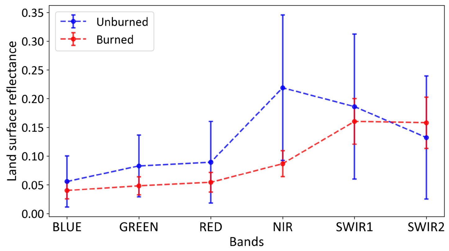
2.4. Sensitive Features for Burned Surfaces
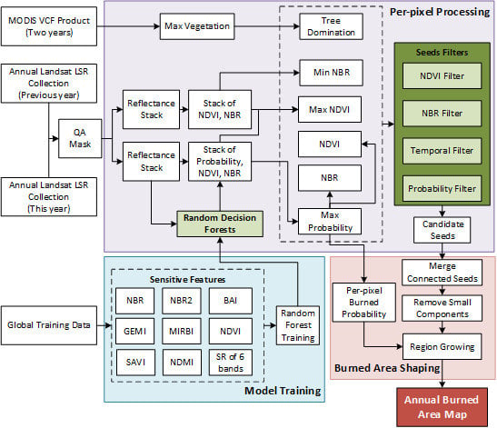
2.5. Burned Area Mapping via GEE
2.5.1. Model Training
2.5.2. Per-Pixel Processing
- , the maximum NDVI value within the couple of years should be greater than a threshold . We choose NDVI as it has been found to be a good identifier of vigorous vegetation, and this constraint is used to exclude areas that appeared as burned, but in fact were just lacking vegetation.
- , the difference between the maximum NDVI and the NDVI when the pixel was most like a burned scar should be greater than a threshold . This constraint ensures evidence of vegetation decrease when the burn happened.
- , the NBR value of a burned pixel should be less than the minimum NBR of the previous year, and the threshold is the minimum acceptable decline of NBR. This constraint is useful to exclude false detections with periodic variation of NBR and NDVI, such as mountain shadows, burned-like soil in deciduous season, snow melting, and flooding.
- or , the date when the vegetation becomes greenest should be earlier than the burning date or the lagged days should be greater than a threshold . For a tree-covered surface, it usually takes a long time for the vegetation to recover more flourishing than the previous year, thus the burn-like pixels with are likely attributed to a false alarm. However, as the recovering of burned trees can be fast in tropic regions, high post-fire regrowth within a reasonable amount of days is also acceptable.
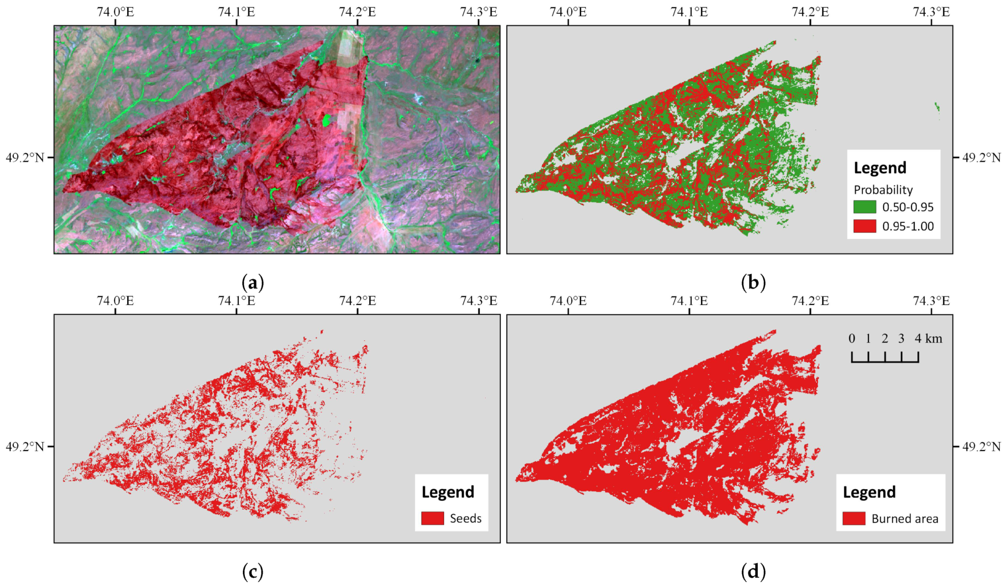
2.5.3. Burned Area Shaping
2.6. Comparison with the Fire_cci Product
2.7. Validation
2.7.1. Data Sources
2.7.2. Reference Data Generation
- PreprocessingAll the images utilized to generate BA reference data were spatially aligned with a mean squared error of less than 1 pixel. The ortho-rectified LC8 and CB4 images met the requirement of geometric accuracy, yet the GF1 images did not. Accordingly, an automated method [52] was applied to orthorectify the time-series GF1 images, taking the LC8 panchromatic images (spatial resolution was 15 m) as geo-references.
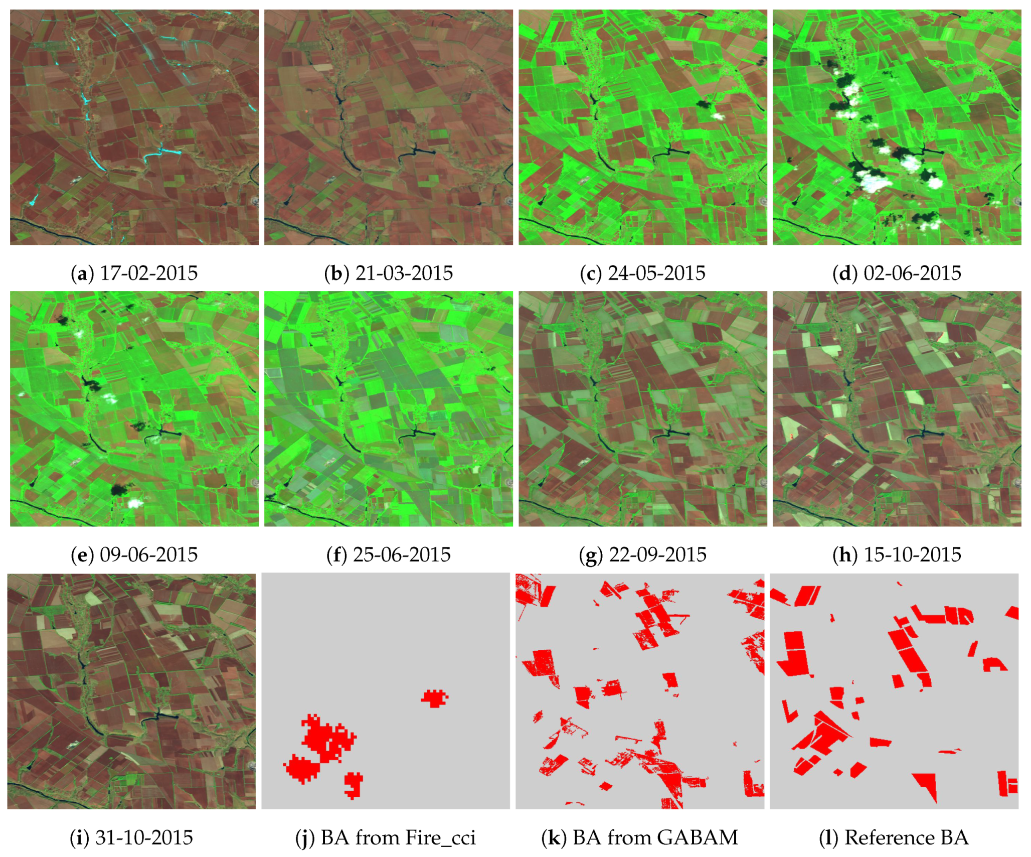
- BA detectionBA perimeters were generated from the time-series images via a semi-automatic approach. Firstly, image pairs (pre- and post-fire) were manually selected from the time-series image by checking whether any new burned scars appeared in the newer images. For LC8 images, SWIR2, NIR, and green bands were composited in a Red, Green, Blue (RGB) combination; for CB4 and GF1 images, red, NIR, and green bands were composited in an RGB combination. The identification of BA might be difficult for CB4 and GF1 images due to the lack of shortwave infrared bands; thus, the Fire_cci BA product was used to verify the BA identification. Secondly, burned and unburned samples were manually collected from each selected image pair. The burned samples included only the newly-burned scars, which appeared burned in the newer image, but unburned in the older image; the unburned samples consisted of unburned pixels, partially recovered BA pixels, and also pixels covered by cloud or cloud shadows in either images. Afterwards, the Support Vector Machines (SVM) classifier in ENVITM (provided by Harris Geospatial in Broomfield, CO, United States) software was used to classify each image pair into burned and unburned pixels, and the detected burned pixels in all the image pairs were integrated to create a composited annual BA map. Note that the sensitive features in Section 2.4 were utilized in SVM for each LC8 image pair; but for CB4 and GF1 images, the features used for classification consisted of the Digital Number (DN) values in four bands of an image pair (in total, 8 DN values), as most of the burned-sensitive spectral indices cannot be derived from the RGB-NIR bands. Finally, the BA perimeters of 2015 were generated from the annual BA composition using the vectorization tool in ArcGISTM (provided by Environmental Systems Research Institute in Redlands, CA, United States) software.
- Reviewing and manually revisionThe result of the supervised classifier (SVM) and automated vectorization algorithm might not be perfect; thus, BA perimeters were further edited visually by experienced experts, via overlapping the vector layer of BA perimeters with the satellite image layers.
2.7.3. Assessment
- Commission error (): , the ratio between the false BA positives (detected burned areas that were not in fact burned) and the total area classified as burned by GABAM 2015.
- Omission error (): , the ratio between the false BA negatives (actual burned areas not detected) and the total area classified as burned by the reference data.
- Overall accuracy (): , the ratio between the area classified correctly and the total area to evaluate.
3. Results and Analysis
3.1. Product Description
3.2. Comparison with the Fire_cci Product
3.2.1. Visual Comparison
3.2.2. Global Grid Map
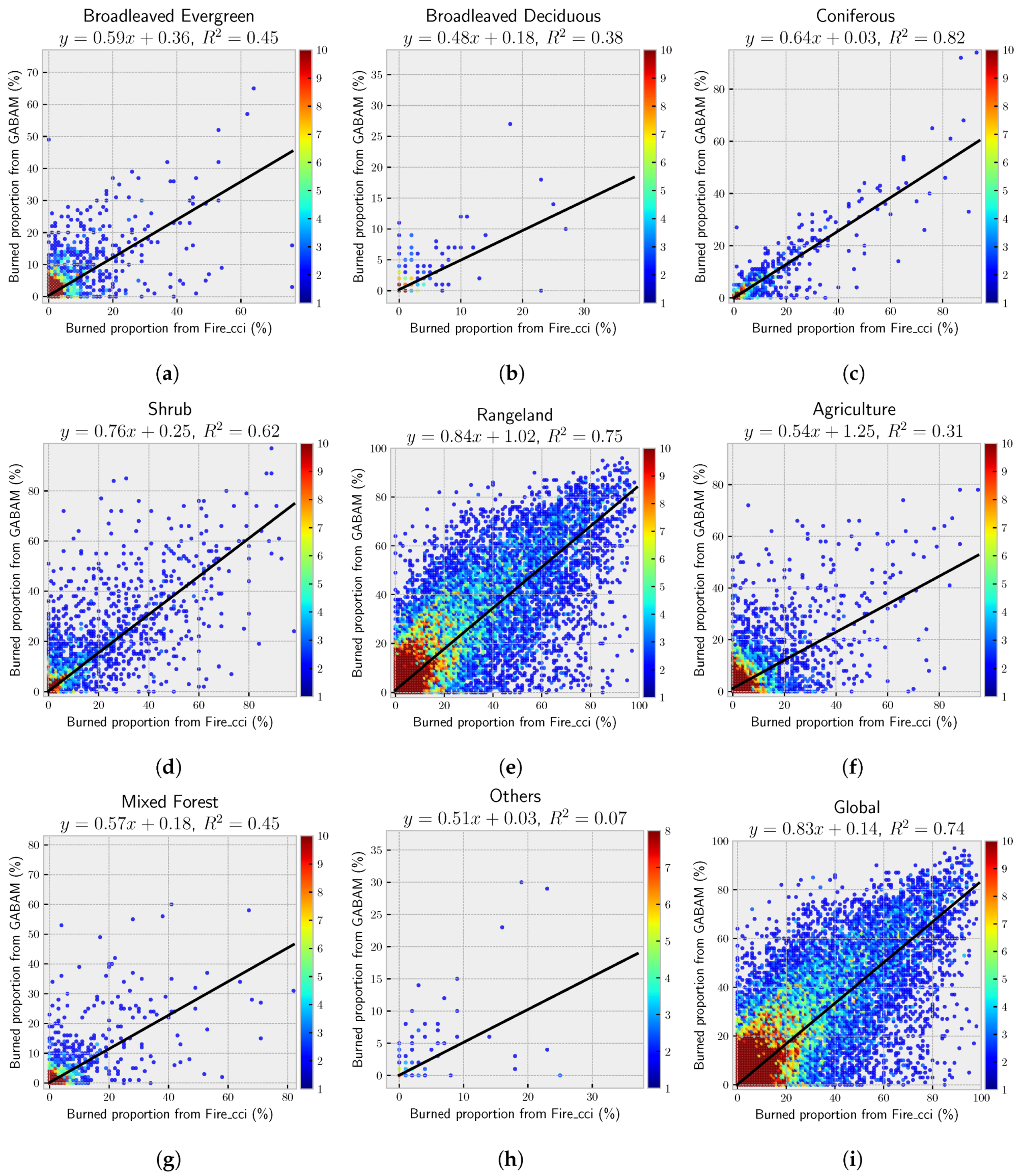
3.2.3. Regression Analysis
3.3. Validation
- In the validation sites located in tropical zones, clear burned evidence was frequently missed by the Landsat sensor due to the quick recovery of the vegetation surface. This point will be further discussed in Section 4.
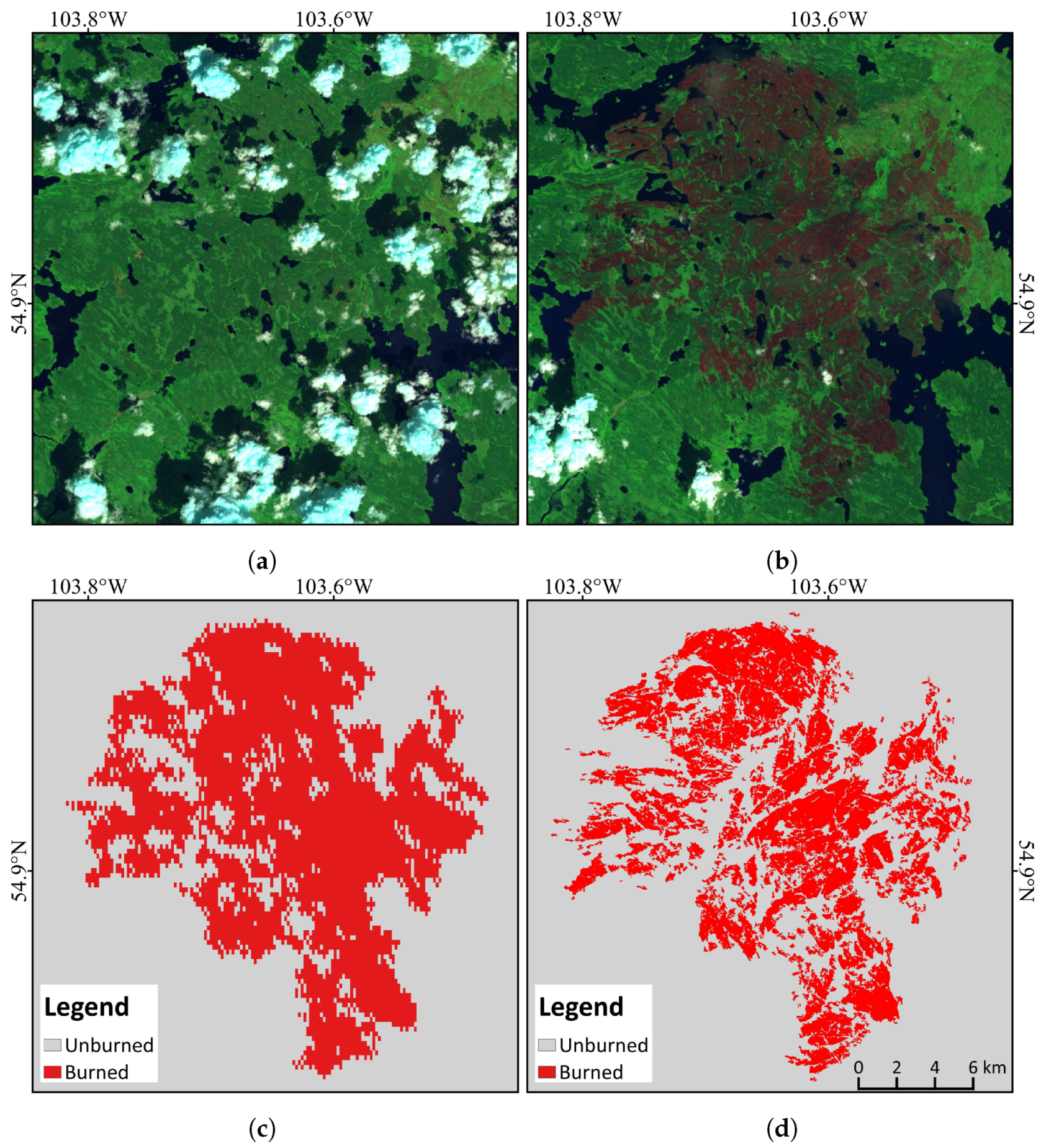
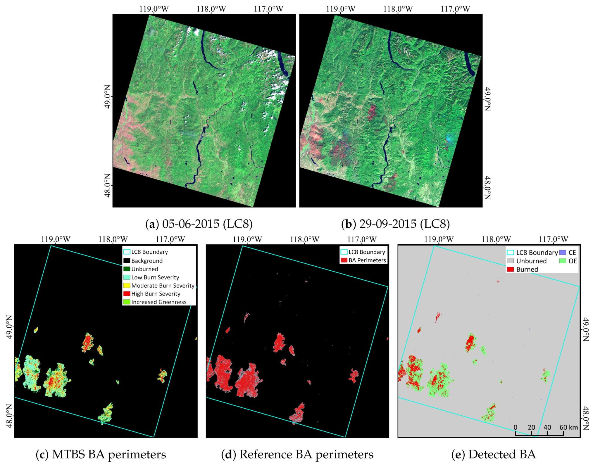
- Some pixels located within a burned area, but not showing a strong burned appearance, might be excluded by GABAM 2015 (e.g., Figure 7d), while they were considered as a part of a complete burned scar in the reference data. Particularly, high was found at those validation sites using MTBS perimeters, e.g., the and of the validation site in Figure A5 were 1.45% and 67.97%. Furthermore, this high omission error might result from the high commission error associated with MTBS perimeters [56].
4. Discussion
4.1. BA in Agriculture Land
- Many croplands have comparable spectral characteristics to burned areas when harvested or ploughed.
- The temporal behavior of harvest or burning of cropland is similar to that of grassland fire, e.g., sudden decline and gradual recovery of NDVI, as well as periodic variation of NBR values year after year.
- Different from the wildfires in rangeland and forest, most of the fires in croplands are human-intended stubble burning, and they are commonly small and of a short duration, being difficult to capture by satellite sensors. In this sense, the traditional burned area detection algorithms, which are frequently used to generate BA products from the data source of a medium resolution (e.g., MODIS, AVHRR, MERIS), are likely to have high omission error in croplands for small cropland fire.
4.2. Omission of Observations
4.3. Validation
5. Conclusions
Author Contributions
Funding
Conflicts of Interest
Appendix A. Examples of Validation Sites

| ID | Location | Reference Data | (%) | (%) | (%) | Figure |
|---|---|---|---|---|---|---|
| 1 | China | GF1 | 7.23 | 10.56 | 91.75 | Figure A1 |
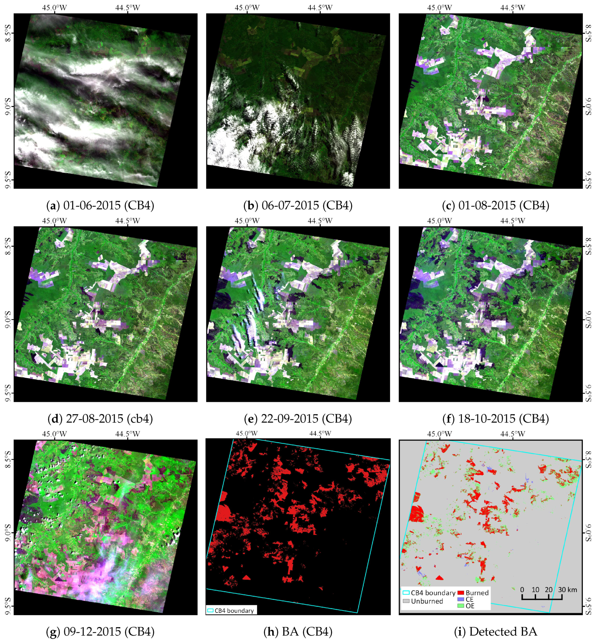
| 2 | South America | CB4 | 13.95 | 33.25 | 94.88 | Figure A2 |
| 3 | Africa | LC8 | 41.23 | 57.41 | 71.29 | Figure A3 |
| 4 | Australia | LC8 | 0.77 | 20.88 | 90.22 | Figure A4 |
| 5 | U.S. | LC8 & MTBS | 1.45 | 67.97 | 95.87 | Figure A5 |


References
- Chuvieco, E.; Yue, C.; Heil, A.; Mouillot, F.; Alonso-Canas, I.; Padilla, M.; Pereira, J.M.; Oom, D.; Tansey, K. A new global burned area product for climate assessment of fire impacts. Glob. Ecol. Biogeogr. 2016, 25, 619–629. [Google Scholar] [CrossRef]
- Carmona-Moreno, C.; Belward, A.; Malingreau, J.P.; Hartley, A.; Garcia-Alegre, M.; Antonovskiy, M.; Buchshtaber, V.; Pivovarov, V. Characterizing interannual variations in global fire calendar using data from Earth observing satellites. Glob. Chang. Biol. 2005, 11, 1537–1555. [Google Scholar] [CrossRef]
- Tansey, K. Vegetation burning in the year 2000: Global burned area estimates from SPOT VEGETATION data. J. Geophys. Res. 2004, 109. [Google Scholar] [CrossRef]
- Simon, M. Burnt area detection at global scale using ATSR-2: The GLOBSCAR products and their qualification. J. Geophys. Res. 2004, 109. [Google Scholar] [CrossRef]
- Plummer, S.; Arino, O.; Simon, M.; Steffen, W. Establishing A Earth Observation Product Service for the Terrestrial Carbon Community: The Globcarbon Initiative. Mitig. Adapt. Strateg. Glob. Chang. 2006, 11, 97–111. [Google Scholar] [CrossRef]
- Tansey, K.; Grégoire, J.M.; Defourny, P.; Leigh, R.; Pekel, J.F.; van Bogaert, E.; Bartholomé, E. A new, global, multi-annual (2000–2007) burnt area product at 1 km resolution. Geophys. Res. Lett. 2008, 35. [Google Scholar] [CrossRef]
- Roy, D.; Jin, Y.; Lewis, P.; Justice, C. Prototyping a global algorithm for systematic fire-affected area mapping using MODIS time-series data. Remote Sens. Environ. 2005, 97, 137–162. [Google Scholar] [CrossRef]
- Giglio, L.; Randerson, J.T.; van der Werf, G.R.; Kasibhatla, P.S.; Collatz, G.J.; Morton, D.C.; DeFries, R.S. Assessing variability and long-term trends in burned area by merging multiple satellite fire products. Biogeosciences 2010, 7, 1171–1186. [Google Scholar] [CrossRef]
- Giglio, L.; Schroeder, W.; Justice, C.O. The collection 6 MODIS active fire detection algorithm and fire products. Remote Sens. Environ. 2016, 178, 31–41. [Google Scholar] [CrossRef] [PubMed]
- Chuvieco, E.; Lizundia-Loiola, J.; Pettinari, M.L.; Ramo, R.; Padilla, M.; Tansey, K.; Mouillot, F.; Laurent, P.; Storm, T.; Heil, A.; et al. Generation and analysis of a new global burned area product based on MODIS 250 m reflectance bands and thermal anomalies. Earth Syst. Sci. Data 2018, 10, 2015–2031. [Google Scholar] [CrossRef]
- Pettinari, M.; Chuvieco, E. ESA CCI ECV Fire Disturbance: D3.3.3 Product User Guide—MODIS, version 1.0; ESA Fire-CCI Project; 2018. Available online: http://www.esa-firecci.org/documents (accessed on 21 January 2019).
- Stroppiana, D.; Bordogna, G.; Carrara, P.; Boschetti, M.; Boschetti, L.; Brivio, P. A method for extracting burned areas from Landsat TM/ETM+ images by soft aggregation of multiple Spectral Indices and a region growing algorithm. ISPRS J. Photogramm. Remote Sens. 2012, 69, 88–102. [Google Scholar] [CrossRef]
- Bastarrika, A.; Chuvieco, E.; Martín, M.P. Mapping burned areas from Landsat TM/ETM+ data with a two-phase algorithm: Balancing omission and commission errors. Remote Sens. Environ. 2011, 115, 1003–1012. [Google Scholar] [CrossRef]
- Hawbaker, T.J.; Vanderhoof, M.K.; Beal, Y.J.; Takacs, J.D.; Schmidt, G.L.; Falgout, J.T.; Williams, B.; Fairaux, N.M.; Caldwell, M.K.; Picotte, J.J.; et al. Landsat Burned Area Essential Climate Variable products for the conterminous United States (1984–2015). US Geol. Surv. Data Release 2017. [Google Scholar] [CrossRef]
- Goodwin, N.R.; Collett, L.J. Development of an automated method for mapping fire history captured in Landsat TM and ETM+ time-series across Queensland, Australia. Remote Sens. Environ. 2014, 148, 206–221. [Google Scholar] [CrossRef]
- Eidenshink, J.; Schwind, B.; Brewer, K.; Zhu, Z.L.; Quayle, B.; Howard, S. A Project for Monitoring Trends in Burn Severity. Fire Ecol. 2007, 3, 3–21. [Google Scholar] [CrossRef]
- Alonso-Canas, I.; Chuvieco, E. Global burned area mapping from ENVISAT-MERIS and MODIS active fire data. Remote Sens. Environ. 2015, 163, 140–152. [Google Scholar] [CrossRef]
- Hawbaker, T.J.; Vanderhoof, M.K.; Beal, Y.J.; Takacs, J.D.; Schmidt, G.L.; Falgout, J.T.; Williams, B.; Fairaux, N.M.; Caldwell, M.K.; Picotte, J.J.; et al. Mapping burned areas using dense time-series of Landsat data. Remote Sens. Environ. 2017, 198, 504–522. [Google Scholar] [CrossRef]
- Liu, J.; Heiskanen, J.; Maeda, E.E.; Pellikka, P.K. Burned area detection based on Landsat time-series in savannas of southern Burkina Faso. Int. J. Appl. Earth Observ. Geoinf. 2018, 64, 210–220. [Google Scholar] [CrossRef]
- Gorelick, N.; Hancher, M.; Dixon, M.; Ilyushchenko, S.; Thau, D.; Moore, R. Google Earth Engine: Planetary-scale geospatial analysis for everyone. Remote Sens. Environ. 2017, 202, 18–27. [Google Scholar] [CrossRef]
- Ramo, R.; García, M.; Rodríguez, D.; Chuvieco, E. A data mining approach for global burned area mapping. Int. J. Appl. Earth Observ. Geoinf. 2018, 73, 39–51. [Google Scholar] [CrossRef]
- Key, C.H.; Benson, N.C. The Normalized Burn Ratio (NBR): A Landsat TM Radiometric Measure of Burn Severity; United States Geological Survey, Northern Rocky Mountain Science Center: Bozeman, MT, USA, 1999. [Google Scholar]
- Lutes, D.C.; Keane, R.E.; Caratti, J.F.; Key, C.H.; Benson, N.C.; Sutherland, S.; Gangi, L.J. FIREMON: Fire Effects Monitoring and Inventory System; Gen. Tech. Rep. RMRS-GTR-164-CD; US Department of Agriculture, Forest Service, Rocky Mountain Research Station: Fort Collins, CO, USA, 2006; Volume 1. [Google Scholar]
- Martín, M. Cartografía e Inventario de Incendios Forestales en la Península Ibérica a Partir de Imágenes NOAA-AVHRR; Departmento de Geografía. Alcalá de Henares, Universidad de Alcalá: Madrid, Spain, 1998. [Google Scholar]
- Trigg, S.; Flasse, S. An evaluation of different bi-spectral spaces for discriminating burned shrub-savannah. Int. J. Remote Sens. 2001, 22, 2641–2647. [Google Scholar] [CrossRef]
- Stroppiana, D.; Boschetti, M.; Zaffaroni, P.; Brivio, P. Analysis and Interpretation of Spectral Indices for Soft Multicriteria Burned-Area Mapping in Mediterranean Regions. IEEE Geosci. Remote Sens. Lett. 2009, 6, 499–503. [Google Scholar] [CrossRef]
- Pinty, B.; Verstraete, M.M. GEMI: A non-linear index to monitor global vegetation from satellites. Vegetatio 1992, 101, 15–20. [Google Scholar] [CrossRef]
- Pereira, J. A comparative evaluation of NOAA/AVHRR vegetation indexes for burned surface detection and mapping. IEEE Trans. Geosci. Remote Sens. 1999, 37, 217–226. [Google Scholar] [CrossRef]
- Huete, A. A soil-adjusted vegetation index (SAVI). Remote Sens. Environ. 1988, 25, 295–309. [Google Scholar] [CrossRef]
- Veraverbeke, S.; Gitas, I.; Katagis, T.; Polychronaki, A.; Somers, B.; Goossens, R. Assessing post-fire vegetation recovery using red–near infrared vegetation indices: Accounting for background and vegetation variability. ISPRS J. Photogramm. Remote Sens. 2012, 68, 191. [Google Scholar] [CrossRef]
- Wilson, E.H.; Sader, S.A. Detection of forest harvest type using multiple dates of Landsat TM imagery. Remote Sens. Environ. 2002, 80, 385–396. [Google Scholar] [CrossRef]
- Friedl, M.; Sulla-Menashe, D. MCD12C1 MODIS/Terra+Aqua Land Cover Type Yearly L3 Global 0.05Deg CMG. 2015. Available online: https://lpdaac.usgs.gov/dataset_discovery/modis/modis_products_table/mcd12c1 (accessed on 21 January 2019).
- Giglio, L.; Randerson, J.T.; van der Werf, G.R. Analysis of daily, monthly, and annual burned area using the fourth-generation global fire emissions database (GFED4). J. Geophys. Res. Biogeosci. 2013, 118, 317–328. [Google Scholar] [CrossRef]
- DAAC, N.L. MODIS Vegetation Continuous Fields (VCF) Product. Version 5.1. 2015. Available online: https://lpdaac.usgs.gov/dataset_discovery/modis/modis_products_table/mod44b (accessed on 21 January 2019).
- Zhu, Z.; Woodcock, C.E. Automated cloud, cloud shadow, and snow detection in multitemporal Landsat data: An algorithm designed specifically for monitoring land cover change. Remote Sens. Environ. 2014, 152, 217–234. [Google Scholar] [CrossRef]
- Boschetti, L.; Roy, D.; Justice, C. International Global Burned Area Satellite Product Validation Protocol (Part I–production and standardization of validation reference data). In CEOS-CalVal; Committee on Earth Observation Satellites: Silver Spring, MD, USA, 2009; pp. 1–11. [Google Scholar]
- Vanderhoof, M.K.; Fairaux, N.; Beal, Y.J.G.; Hawbaker, T.J. Validation of the USGS Landsat Burned Area Essential Climate Variable (BAECV) across the conterminous United States. Remote Sens. Environ. 2017, 198, 393–406. [Google Scholar] [CrossRef]
- Padilla, M.; Stehman, S.V.; Ramo, R.; Corti, D.; Hantson, S.; Oliva, P.; Alonso-Canas, I.; Bradley, A.V.; Tansey, K.; Mota, B.; et al. Comparing the accuracies of remote sensing global burned area products using stratified random sampling and estimation. Remote Sens. Environ. 2015, 160, 114–121. [Google Scholar] [CrossRef]
- Boschetti, L.; Stehman, S.V.; Roy, D.P. A stratified random sampling design in space and time for regional to global scale burned area product validation. Remote Sens. Environ. 2016, 186, 465–478. [Google Scholar] [CrossRef] [PubMed]
- Padilla, M.; Olofsson, P.; Stehman, S.V.; Tansey, K.; Chuvieco, E. Stratification and sample allocation for reference burned area data. Remote Sens. Environ. 2017, 203, 240–255. [Google Scholar] [CrossRef]
- Chuvieco, E.; Padilla, M.; Hantson, S.; Theis, R.; Snadow, C. ESA CCI ECV Fire Disturbance-Product Validation Plan (v3.1); ESA Fire-CCI Project; 2011. Available online: http://www.esa-fire-cci.org/ (accessed on 21 January 2019).
- Padilla, M.; Stehman, S.V.; Chuvieco, E. Validation of the 2008 MODIS-MCD45 global burned area product using stratified random sampling. Remote Sens. Environ. 2014, 144, 187–196. [Google Scholar] [CrossRef]
- Vermote, E.; Justice, C.; Claverie, M.; Franch, B. Preliminary analysis of the performance of the Landsat 8/OLI land surface reflectance product. Remote Sens. Environ. 2016, 185, 46–56. [Google Scholar] [CrossRef]
- Koutsias, N.; Karteris, M. Burned area mapping using logistic regression modeling of a single post-fire Landsat-5 Thematic Mapper image. Int. J. Remote Sens. 2000, 21, 673–687. [Google Scholar] [CrossRef]
- Bastarrika, A.; Alvarado, M.; Artano, K.; Martinez, M.; Mesanza, A.; Torre, L.; Ramo, R.; Chuvieco, E. BAMS: A Tool for Supervised Burned Area Mapping Using Landsat Data. Remote Sens. 2014, 6, 12360–12380. [Google Scholar] [CrossRef]
- Boschetti, M.; Stroppiana, D.; Brivio, P.A. Mapping Burned Areas in a Mediterranean Environment Using Soft Integration of Spectral Indices from High-Resolution Satellite Images. Earth Interact. 2010, 14, 1–20. [Google Scholar] [CrossRef]
- Boschetti, L.; Roy, D.P.; Justice, C.O.; Humber, M.L. MODIS–Landsat fusion for large area 30m burned area mapping. Remote Sens. Environ. 2015, 161, 27–42. [Google Scholar] [CrossRef]
- Sobrino, J.A.; Raissouni, N. Toward remote sensing methods for land cover dynamic monitoring: Application to Morocco. Int. J. Remote Sens. 2000, 21, 353–366. [Google Scholar] [CrossRef]
- Miller, J.D.; Thode, A.E. Quantifying burn severity in a heterogeneous landscape with a relative version of the delta Normalized Burn Ratio (dNBR). Remote Sens. Environ. 2007, 109, 66–80. [Google Scholar] [CrossRef]
- Lhermitte, S.; Verbesselt, J.; Verstraeten, W.; Veraverbeke, S.; Coppin, P. Assessing intra-annual vegetation regrowth after fire using the pixel based regeneration index. ISPRS J. Photogramm. Remote Sens. 2011, 66, 17–27. [Google Scholar] [CrossRef]
- Laris, P.S. Spatiotemporal problems with detecting and mapping mosaic fire regimes with coarse-resolution satellite data in savanna environments. Remote Sens. Environ. 2005, 99, 412–424. [Google Scholar] [CrossRef]
- Long, T.; Jiao, W.; He, G.; Zhang, Z. A Fast and Reliable Matching Method for Automated Georeferencing of Remotely-Sensed Imagery. Remote Sens. 2016, 8, 56. [Google Scholar] [CrossRef]
- Pontius, R.G.; Millones, M. Death to Kappa: Birth of quantity disagreement and allocation disagreement for accuracy assessment. Int. J. Remote Sens. 2011, 32, 4407–4429. [Google Scholar] [CrossRef]
- Cochran, W.G. Sampling Techniques; John Wiley & Sons: Hoboken, NJ, USA, 2007. [Google Scholar]
- Moritz, H. Geodetic reference system 1980. Bulletin Géodésique 1980, 54, 395–405. [Google Scholar] [CrossRef]
- Sparks, A.M.; Boschetti, L.; Smith, A.M.; Tinkham, W.T.; Lannom, K.O.; Newingham, B.A. An accuracy assessment of the MTBS burned area product for shrub–steppe fires in the northern Great Basin, United States. Int. J. Wildl. Fire 2015, 24, 70–78. [Google Scholar] [CrossRef]
- Strahler, A.H.; Boschetti, L.; Foody, G.M.; Friedl, M.A.; Hansen, M.C.; Herold, M.; Mayaux, P.; Morisette, J.T.; Stehman, S.V.; Woodcock, C.E. Global Land Cover Validation: Recommendations for Evaluation and Accuracy Assessment of Global land Cover Maps; European Communities: Luxembourg, 2006; Volume 51. [Google Scholar]


| Data | Usage | Source |
|---|---|---|
| MCD12C1 [32] | Stratified sampling for type of land cover | https://e4ftl01.cr.usgs.gov/MOTA/MCD12C1.006/ |
| GFED4 [33] | Stratified sampling for fire frequency | https://www.globalfiredata.org/data.html |
| Landsat-8 | BA mapping and validation | https://code.earthengine.google.com/dataset/LANDSAT/LC08/C01/T2_SR https://code.earthengine.google.com/dataset/LANDSAT/LC08/C01/T1_SR |
| MOD44B [34] | Adjustment constraint conditions for BA mapping | https://code.earthengine.google.com/dataset/MODIS/051/MOD44B |
| Fire_cci v5 [11] | Comparison | https://geogra.uah.es/fire_cci |
| CBERS-4 MUX | Validation | http://www.dgi.inpe.br/catalogo/ |
| Gaofen-1 WFV | Validation | http://218.247.138.119:7777/DSSPlatform/productSearch.html |
| MTBS [16] | Validation | https://www.mtbs.gov/direct-download |
| Sensors | Spatial Resolution at Nadir (m) | Swath Width at Nadir (km) | Spectral Bands (m) | |||
|---|---|---|---|---|---|---|
| Blue | Green | Red | NIR | |||
| CBERS-4 MUX | 20 | 120 | 0.45–0.52 | 0.52–0.59 | 0.63–0.69 | 0.77–0.89 |
| Gaofen-1 WFV | 16 | 192 | ||||
| New Classification | Original UMD Type |
|---|---|
| Broadleaved Evergreen | Evergreen Broadleaf Forest |
| Broadleaved Deciduous | Deciduous Broadleaf Forest |
| Coniferous | Evergreen Needleleaf Forest |
| Deciduous Needleleaf Forest | |
| Mixed Forest | Mixed Forest |
| Shrub | Closed Shrublands |
| Open Shrublands | |
| Rangeland | Woody Savannas |
| Savannas | |
| Grasslands | |
| Agriculture | Croplands |
| Others | Water |
| Urban and Built-up | |
| Barren or Sparsely Vegetated |
| Land Cover Type | Training Sample Count | Validation Sample Count |
|---|---|---|
| Broadleaved Evergreen | 16 | 11 |
| Broadleaved Deciduous | 12 | 9 |
| Coniferous | 13 | 9 |
| Mixed Forest | 12 | 8 |
| Shrub | 18 | 12 |
| Rangeland | 25 | 15 |
| Agriculture | 24 | 16 |
| Name | Abbreviation | Reference | Formula |
|---|---|---|---|
| Normalized Burned Ratio | NBR | Key and Benson [22] | |
| Normalized Burned Ratio 2 | NBR2 | Lutes et al. [23] | |
| Burned Area Index | BAI | Martín [24] | |
| Mid-Infrared Burn Index | MIRBI | Trigg and Flasse [25] | |
| Normalized Difference Vegetation Index | NDVI | Stroppiana et al. [26] | |
| Global Environmental Monitoring Index | GEMI | Pinty and Verstraete [27] | , |
| Soil-Adjusted Vegetation Index | SAVI | Huete [29] | , |
| Normalized Difference Moisture Index | NDMI | Wilson and Sader [31] |
| Reference Data (pixel) | ||||
|---|---|---|---|---|
| Burned | Unburned | Total | ||
| GABAM 2015 (pixel) | Burned | |||
| Unburned | ||||
| Total | ||||
| Land Cover Type | (%) | (%) | (%) | (%) | (%) | (%) |
|---|---|---|---|---|---|---|
| Broadleaved Evergreen | 8.64 | 10.95 | 90.99 | 9.14 | 16.52 | 6.78 |
| Broadleaved Deciduous | 23.59 | 34.85 | 99.03 | 12.33 | 19.16 | 7.22 |
| Coniferous | 7.41 | 18.27 | 99.77 | 11.47 | 16.15 | 6.00 |
| Mixed Forest | 8.73 | 34.33 | 98.36 | 9.30 | 24.19 | 8.41 |
| Shrub | 13.00 | 3.78 | 99.49 | 11.05 | 16.05 | 8.78 |
| Rangeland | 11.91 | 23.06 | 91.79 | 13.55 | 17.91 | 9.04 |
| Agriculture | 10.91 | 45.38 | 94.41 | 10.50 | 28.09 | 7.33 |
© 2019 by the authors. Licensee MDPI, Basel, Switzerland. This article is an open access article distributed under the terms and conditions of the Creative Commons Attribution (CC BY) license (http://creativecommons.org/licenses/by/4.0/).
Share and Cite
Long, T.; Zhang, Z.; He, G.; Jiao, W.; Tang, C.; Wu, B.; Zhang, X.; Wang, G.; Yin, R. 30 m Resolution Global Annual Burned Area Mapping Based on Landsat Images and Google Earth Engine. Remote Sens. 2019, 11, 489. https://doi.org/10.3390/rs11050489
Long T, Zhang Z, He G, Jiao W, Tang C, Wu B, Zhang X, Wang G, Yin R. 30 m Resolution Global Annual Burned Area Mapping Based on Landsat Images and Google Earth Engine. Remote Sensing. 2019; 11(5):489. https://doi.org/10.3390/rs11050489
Chicago/Turabian StyleLong, Tengfei, Zhaoming Zhang, Guojin He, Weili Jiao, Chao Tang, Bingfang Wu, Xiaomei Zhang, Guizhou Wang, and Ranyu Yin. 2019. "30 m Resolution Global Annual Burned Area Mapping Based on Landsat Images and Google Earth Engine" Remote Sensing 11, no. 5: 489. https://doi.org/10.3390/rs11050489
APA StyleLong, T., Zhang, Z., He, G., Jiao, W., Tang, C., Wu, B., Zhang, X., Wang, G., & Yin, R. (2019). 30 m Resolution Global Annual Burned Area Mapping Based on Landsat Images and Google Earth Engine. Remote Sensing, 11(5), 489. https://doi.org/10.3390/rs11050489