Spectral Reflectance Modeling by Wavelength Selection: Studying the Scope for Blueberry Physiological Breeding under Contrasting Water Supply and Heat Conditions

Abstract

To overcome the environmental changes occurring now and predicted for the future, it is essential that fruit breeders develop cultivars with better physiological performance. During the last few decades, high-throughput plant phenotyping and phenomics have been developed primarily in cereal breeding programs. In this study, plant reflectance, at the level of the leaf, was used to assess several physiological traits in five Vaccinium spp. cultivars growing under four controlled conditions (no-stress, water deficit, heat stress, and combined stress). Two modeling methodologies [Multiple Linear Regression (MLR) and Partial Least Squares (PLS)] with or without (W/O) prior wavelength selection (multicollinearity, genetic algorithms, or in combination) were considered. PLS generated better estimates than MLR, although prior wavelength selection improved MLR predictions. When data from the environments were combined, PLS W/O gave the best assessment for most of the traits, while in individual environments, the results varied according to the trait and methodology considered. The highest validation predictions were obtained for chlorophyll a/b (R²_Val ≤ 0.87), maximum electron transport rate (R²_Val ≤ 0.60), and the irradiance at which the electron transport rate is saturated (R²_Val ≤ 0.59). The results of this study, the first to model modulated chlorophyll fluorescence by reflectance, confirming the potential for implementing this tool in blueberry breeding programs, at least for the estimation of a number of important physiological traits. Additionally, the differential effects of the environment on the spectral signature of each cultivar shows this tool could be directly used to assess their tolerance to specific environments.

1. Introduction

Agriculture is essential to human survival, but it is being critically affected by global warming, compromising the food security of the population that is predicted to continue to increase over the coming decades [1]. Elevated temperatures, changes in precipitation patterns and more frequent extreme weather events have given rise to greater intra- and inter-annual variability in the yield and quality of crops [2]. These new climatic scenarios make it necessary to further our understanding of the principal projected stresses (drought and heat stress) impacting plant performance, and to develop relevant information to generate cultivars capable of overcoming more complex environmental scenarios.

To the extent that breeders can consider useful additional information (e.g., plant physiology) to plan each season’s crosses and perform early selection of material suitable for each breeding program’s aims, it should be possible to improve both efficiency (cost and time) and productivity (higher proportion of new cultivars carrying advantageous characteristics) [3,4].

Unfortunately, the practical and economic limitations of performing complex evaluations (e.g., plant water status, photosystem status, leaf gas exchange, photosynthetic pigment contents) of a large number of genotypes has been one of the main constraints to performing in-depth phenotypic characterization, especially under water deficit or heat stress conditions [3,5,6]. This highlights the urgent need to develop faster and cheaper methodologies to estimate key physiological traits, which have proven to be relevant in the multi-dimensional characterization of the phenotype (phenomics) [7], especially in fruit breeding programs [3]. Nevertheless, it is important to highlight that these new technologies need to be calibrated and validated; therefore, they must first be developed in conjunction with reference traditional measures to establish correlations and the degree of realistic predictability.

Among the remote sensing technologies with potential for high-throughput plant phenotyping and phenomics, reflectance spectroscopy is probably the most promising. When the leaf receives radiation of the sun, part is transmitted to lower leaf layers, part is absorbed by the chlorophylls and other pigments, and the rest is reflected; the reflectance is therefore the ratio of the reflected and incident radiation. The spectral signature (graphical representation of the reflectance for each wavelength) is closely associated with the absorption of certain wavelengths linked to specific characteristics or plant conditions [8,9,10,11]; plant spectral reflectance can thus be used for characterizing the effects of abiotic and biotic stresses [3,9,12,13]. For example, in a healthy leaf, chlorophyll pigments absorb in the blue (400–500 nm) and red (600–700 nm) range, generating a higher reflection in the green wavelengths (500–600 nm); carotene has also a strong absorbance in the blue range. Most of the past research has concentrated on the measurement in the visible (VIS; ~400–770 nm) and near infrared (NIR; ~770–1300 nm) spectrum, although new studies are also covering the UV (~300–400 nm) and the short wavelength infrared 1 (SWIR1; ~1300–1900 nm) and 2 (SWIR2; ~1900–2500 nm) [14,15].

Reflectance spectroscopy has gained importance and is being widely used in eco-physiological studies for predicting traits of interest [10,16]. However, most of the studies have focused on the use of Spectral Reflectance Indices (SRIs) (denoting relationships between specific wavelengths or spectrum bands), paying less attention to the use of a wider proportion of wavelengths or the full spectrum [11,17,18,19,20].

Because of the large volume of data generated by spectral measurements, it is common to use multivariate techniques for trait modeling [21]. The simplest method is Multiple Linear Regression (MLR), which is a well-known statistical procedure based on ordinary least squares regression [22,23]. In principle, MLR can be used with many predictors; however, if the number of these becomes too large, it is likely to generate a model that fits the sampled data but has a probability of failing to predict new one, a phenomenon called over-fitting [24,25]. Furthermore, an important assumption for the MLR method is that independent variables are linearly independent, which is not always true for spectral data due to multicollinearity (MC). One alternative to MLR is the use of Partial Least Squares (PLS), which is a bilinear modeling method where information in the original x variables is projected onto a small number of latent variables called PLS components; characteristics of principal component analysis and multiple linear regression are used to reduce the complex variability to some smaller number of relevant factors [26,27,28]. PLS is thus a method for constructing predictive models when there are many factors and high multicollinearity.

To avoid problems associated with MLR models in spectral studies, prior to the modeling it is suggested that a selection of predictors is used to reduce their number, leaving only those that contribute most to the model. Due to spectral data characteristics, in which one or several sets of predictors provide the same information, the use of an MC analysis contributes towards eliminating those predictors with redundant contributions to the model [29,30]. Another alternative for the selection of independent variables is Genetic Algorithm (GA) analysis, widely used in chemical spectrometry [21,31,32,33,34,35,36,37]. GAs are adaptive procedures for finding solutions, or numerical optimizations, and are inspired by the theory of evolution: in a living environment, the “best” individuals have a greater chance of surviving and a higher probability of spreading their genes by reproduction [38]. In particular, the best chromosomes (with higher fitness) are allowed to survive, mutate and recombine to generate offspring, and after a number of generations have elapsed, only those selected chromosomes (equivalent to sets of wavelengths) are preserved [39].

Despite numerous studies relating the spectral signature (total or partial) to different traits, further investigation is required. A significant number of articles cling to the use of PLS as the principal multivariate technique; nevertheless, comparisons with other methodologies have not always been considered. The literature suggests that modeling with MLR, after selecting wavelengths, would generate models with similar predictive ability to PLS [30,38,40,41]. For example, [42] indicated that the selection of wavelengths with lower MC would improve the performance of MLR models for spectral data with a large number of samples. Questions regarding the best modeling methodology for physiological trait prediction (e.g., PLS vs. MLR), and whether the model should consider the whole spectrum or the convenience of a wavelength selection method still remain unclear.

We propose that it is possible to estimate complex physiological traits using models based on the spectral signature, providing fruit breeders with additional relevant information for plant selection (parents to be crossed or advanced lines) under adverse abiotic conditions (water deficit or heat stress, and their combination). Thus, through the comparison of the coefficients of determination of validation, the aim of this study was to evaluate the potential use of spectral reflectance, at the leaf level, to estimate physiological traits (plant water status, chlorophyll content, leaf gas exchange, and the working state of the photosynthetic apparatus) by determining the performance of PLS and MLR in relation to a previous wavelength selection procedure (GA, MC or in combination). Additionally, a secondary goal was placed on the recognition of the effects of environmental constraints on the leaf spectral signature, considering the differences between and within cultivars.

2. Materials and Methods

2.1. Experimental Trial and Plant Material

The experimental trial was conducted at the Universidad de Talca, Campus Lircay (35° 24′ 20″S, 71° 38′ 5″W), Talca, Chile, in the course of the 2013/14 growing season. During dormancy in the previous year (June 2012), 2- to 3-year-old plants of northern highbush blueberry (Vaccinium corymbosum L.; ‘Bluegold’ and ‘Liberty’), southern highbush blueberry (V. corymbosum L.; ‘Bluecrisp’ and ‘Star’) and rabbiteye (V. ashei Reade; ‘Bonita’) were established in 20 L pots, containing a substrate mixture of sand, peat moss, and sawdust (1:3:1); according to [43], a mature blueberry is shallow-rooting with most roots only exploring up to 0.4 m deep, indicating that the cylinder pot (305 × 383 mm) should provide enough space for a young root system to grow without restrictions. Plants were maintained outdoors until early August 2013 (mid-winter in Chile) when they were moved into two greenhouses (12 × 9 m) covered with alveolar polycarbonate sheeting (6 mm and 86% of solar transmission); one of them (only roof covered) was considered to reproduce the conditions of ambient temperature (at), while the second one, completely enclosed with temperature control set to keep approximately 5 °C above at, simulated an overheated environment (at₊₅) (temperature records in Figure S1). Both greenhouses had two water regimes, full irrigation (FI) and water deficit (WD) with approximately one-third of the water supplied under FI. Therefore, four environmental conditions were generated: (i) at–FI; (ii) at–WD; (iii) at₊₅–FI; and (iv) at₊₅–WD.

There were three benches (blocks) in each greenhouse, and both water regimes were applied to each one. Each individual bench included all cultivars and two replications of each water regime; thus, six plants represented each environmental condition.

2.2. Measurements

Assessments started when 20–30% of the fruit in each cultivar reached maturity (berry skin 100% blue coverage) on each bush. Measurements were performed on fully illuminated tissue (leaves or shoots) from the edge of the middle-third of the canopy, at solar zenith (±2 h) during completely sunny days.

Evaluations of chlorophyll (Chl) content, leaf gas exchange, modulated chlorophyll fluorescence, and spectral reflectance were conducted on the same leaves. Stem water potential (SWP) was measured in shoots of neighboring buds. Descriptions of the measurements are given below:

2.2.1. SWP

Plant water status was assessed on one shoot (15 cm) per plant using a pressure chamber (PMS600, PMS Instruments Company, Corvallis, OR, USA). Prior to the measurement, shoots were covered with aluminum foil and plastic Ziploc^TM bags for two hours [44].

2.2.2. Chl Content

From one leaf per plant, one disc of 0.32 cm² was extracted from each side of the central vein in the middle of the leaf [44]. Both discs were placed in 1.5 ml of the organic solvent N,N-dimethylformamide for 48 h in the dark at 4 °C [45]. The concentrations of Chl a, b and total were determined using a UV/VIS spectrophotometer (T80 +, PG Instruments Ltd., England) at 664.5 and 647 nm, according to the equation proposed by [46]. Additionally, the ratio between Chl a and b (Chl a/b) was calculated.

2.2.3. Leaf Gas Exchange

On one leaf per plant, CO₂ assimilation rate (A), stomatal conductance (gs), transpiration rate (E), and internal CO₂ concentration (Ci) were recorded using an infrared gas analyzer (Ciras 2, PP Systems, Amesbury, MA, USA) with a leaf cuvette of 2.5 cm². Measurements were performed using a light source (CRS131, PP Systems, Amesbury, MA, USA) at saturation conditions (1500 μmol m⁻² s⁻¹), a flow rate of 0.15 L min⁻¹ and 390 ppm of CO₂.

2.2.4. Modulated Chlorophyll Fluorescence:

On one leaf per plant, the working state of the photosynthetic apparatus was evaluated by fast light curves using a portable fluorometer (PAM 2500, Walz, Effeltrich, Germany). The equipment was configured to deliver 20 pulses of actinic light at different levels of photosynthetically active radiation (PAR), between 0 and 2700 μmol m⁻² s⁻¹. The parameters evaluated were those reported by [47], which were useful to discriminate between environments with water deficit and heat stress: effective photochemical quantum yield of photosystem II [Y(II)], coefficient of non-photochemical fluorescence quenching (qN), coefficient of photochemical fluorescence quenching (qP), initial slope of the fast light curve (Alpha), maximum electron transport rate (ETR_max), and the irradiance at which the electron transport rate is saturated (IK), or in other words, the PAR value at the point of intersection of the horizontal line between ETR_max and Alpha.

2.2.5. Spectral reflectance

This was measured using a portable spectrometer (FieldSpec 3 Jr., Analytical Spectral Devices ASD Inc., Boulder, CO, USA) with a spectral range of 350–2500 nm. The spectrometer fiber (25°) was inserted (32°) into a contact probe device (ASD Inc., Boulder, CO, USA) with a halogen light source (5 W to prevent the blade from burning), keeping a constant distance from the leaf (10 mm), and generating a measuring spot of ~10 mm diameter. The contact probe was calibrated every 15 minutes using a white reference tile (Spectralon, ASD Inc., Boulder, CO, USA) for scatter correction. Software RS3 (ASD Inc., Boulder, CO, USA) was used to calibrate, control the spectrometer and to acquire the spectral signatures. The equipment was configured to integrate three samples (350–2500 nm) per scan, and each leaf was scanned ten times. Reflectance data were extracted using View Spec Pro 2008 software (ASD Inc., Boulder, CO, USA). For leaf scan averaging, exploratory analysis of high-resolution spectral reflectance was performed using Spectral Knowledge software (SK-UTALCA) [19].

2.3. Modeling Analysis

Multivariate regression analysis was performed for each of the four individual environments (at–FI, at–WD, at₊₅–FI, and at₊₅–WD), but also considering the four conditions taken together (All). The regression models were developed using MLR (MATLAB, version 7.8.0 R2009a, MathWorks, Inc., Natick, MA, USA) and PLS (The Unscrambler X, version 10.4, Computer Aided Modelling Camo, Trondheim, Norway). PLS was implemented by considering the number of components that maximized the calibration of the models in each analysis. A mean-centering procedure was carried out on all datasets prior to MLR and PLS to remove the offset effect. The validation of each model was evaluated using the methodology of leave-one-out cross-validation (LOO).

Each modeling methodology (PLS or MRL) considered the complete spectral signature (PLS W/O or MLR W/O), which was contrasted with that in which a selection of wavelengths was previously performed by: (i) multicollinearity (MC PLS or MC MLR); (ii) genetic algorithms (GA PLS or GA MLR); (iii) MC and then GA (MC+GA PLS or MC+GA MLR); and (iv) GA and then MC (GA+MC PLS or GA+MC MLR). The final number of wavelengths after each of the selection procedures is given in Table S1.

Using Spectral Knowledge software (SK-UTALCA) [19], MC was established by linear regression analysis, considering a cut-off coefficient of determination of 0.95. Selection by GA was determined by the MATLAB package developed by Leardi (2000), considering the equivalent of the following parameters: population size (30 chromosomes), probability of mutation (1%), probability of crossover (50%), and elitism (1) [10].

As a way to simplify the analysis and discussion of the multiple combinations generated for the study (15 traits, five environmental conditions, two multivariate analyzes, and five wavelength selection methods), only the values of the coefficient of determination for the validation procedure (R²_Val) were considered for the comparisons. Detailed information on the calibration and validation coefficients of determination, and root mean square error (RMSE) of the calibration and validation are given in Table S2.

2.4. Determining the Environmental Effects in the Leaf Spectral Signature

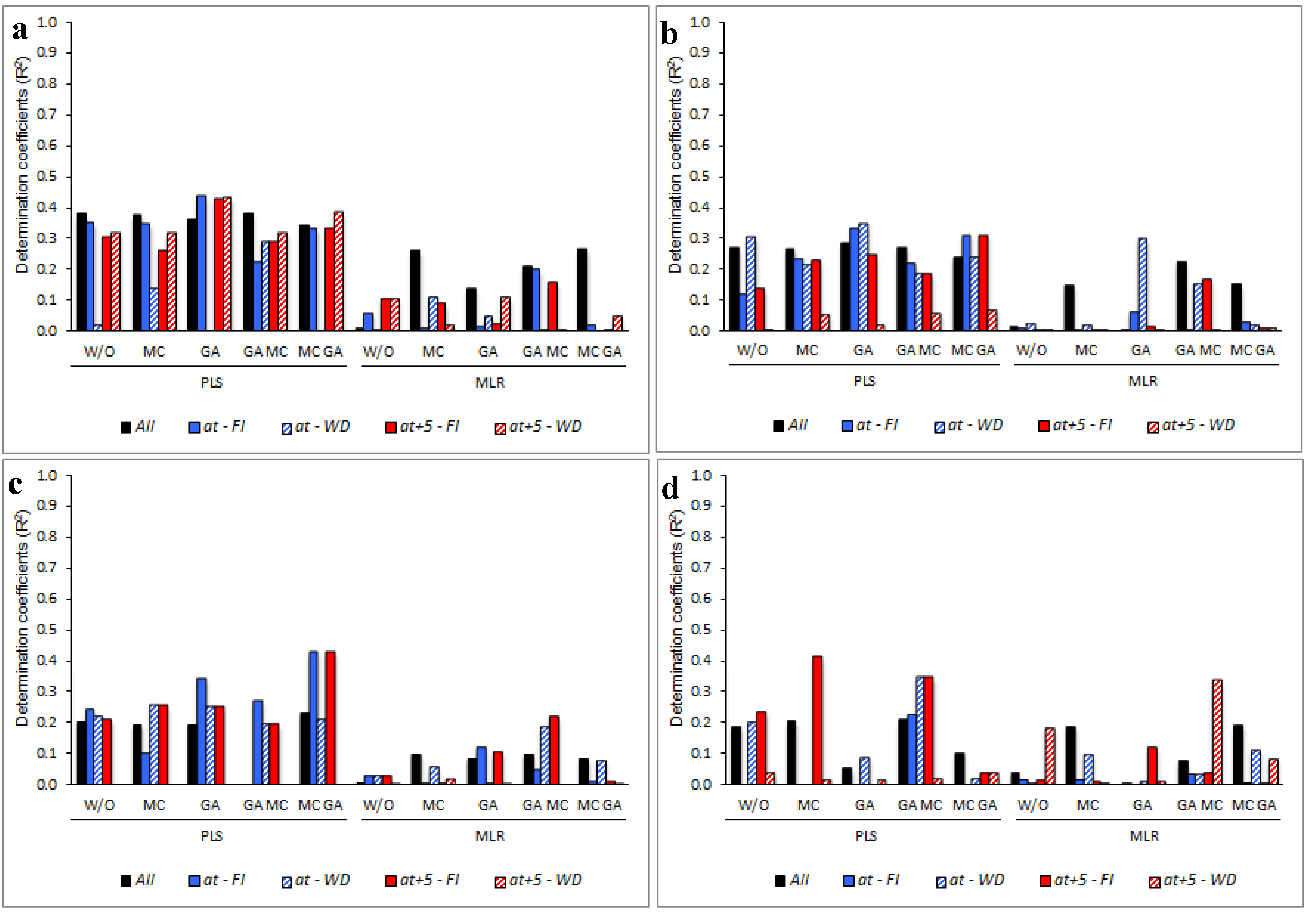
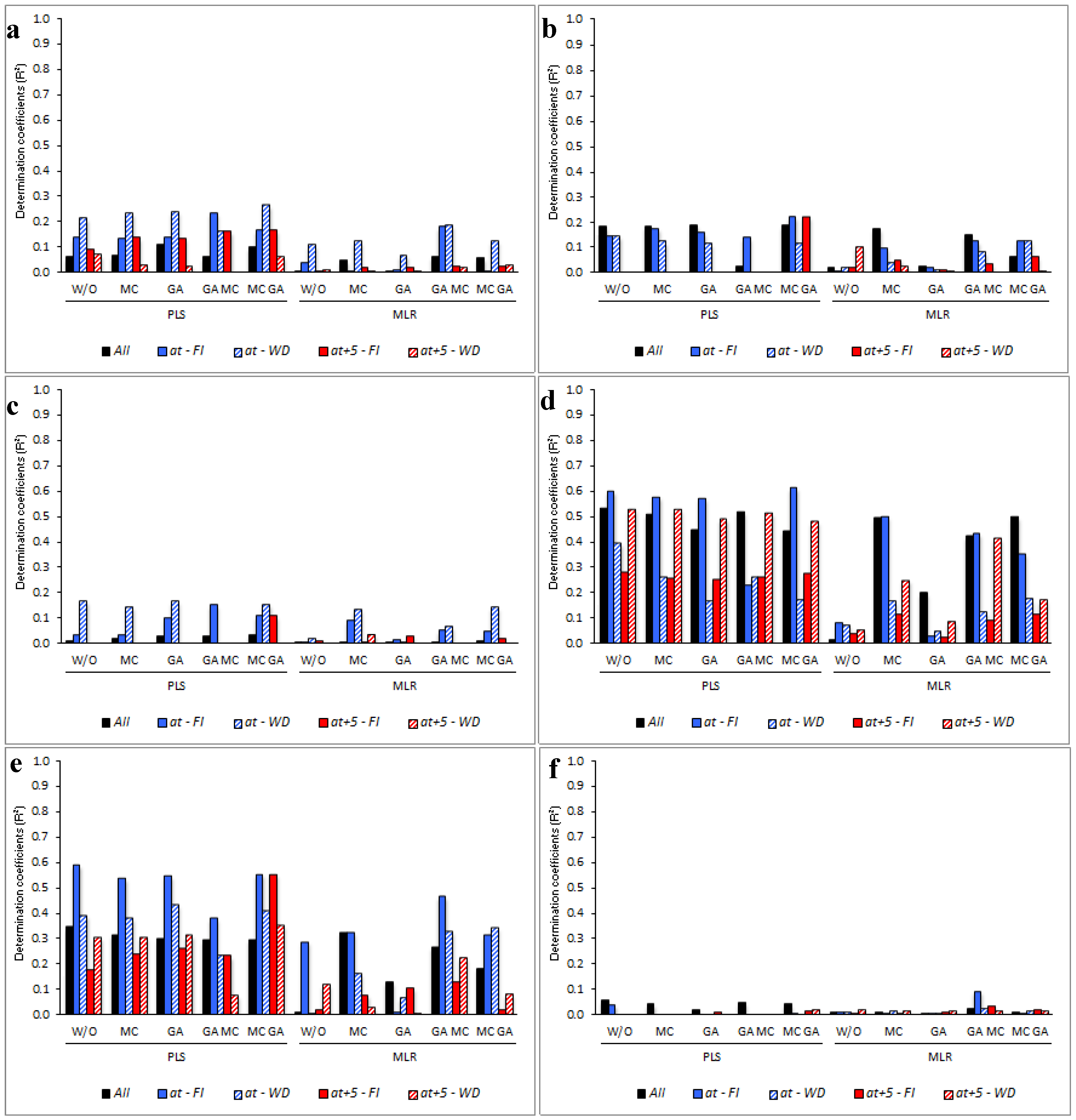
As a way to easily characterize the environmental effects on the spectral signature, magnifying the differences between the compared reflections, a practical methodology is proposed. For each cultivar, the ten scans per leaf were averaged to generate the spectral signature of the replica. Then, the six replicates were also averaged, constituting the spectral signature of the evaluated environment. For each cultivar and wavelength, analyses of variance (ANOVAs) were performed to verify whether the reflectance measurements were statistically different (Table S3).

When statistical differences were found between environments at each wavelength, the average reflectance values of the control treatment and the different adverse conditions (at–WD, at₊₅–FI and at₊₅–WD) were subtracted (at–FI vs. at–WD, at₊₅–FI or at₊₅–WD). Finally, at each wavelength assessed, the reflectance differences between environments were plotted per cultivar.

3. Results

In general, PLS was a better approximation than MLR and this was evident throughout all the analyses. Regardless of the methodology of wavelength selection, the validation models indicated an R²_Val ≥ 0.45, at least in some environments, for SWP, Chl (a, b, total, and a/b), ETR_max and IK (Figure 1, Figure 2, Figure 3 and Figure 4, respectively). When all environmental data were combined (All), in general, the wavelength selection (simple or double) did not improve the estimation by PLS, but it was enhanced under each particular condition (at–FI, at–WD, at₊₅–FI, or at₊₅–WD). At the same time, MLR coefficients of determination of validation increased, particularly when a double selection was considered. In contrast, independent of the modeling methodology and the wavelength selection applied, the worst results obtained were for the estimation of Alpha, qP, qN and Y(II).

3.1. Stem Water Potential (SWP)

PLS performed better than MLR in the prediction of SWP (Figure 1). PLS W/O (full spectrum) showed the best estimation when all environments were considered together (All; R²_Val = 0.29) and under water deficit conditions (at–WD; R²_Val = 0.48). Wavelength selection proved to be an adequate procedure for modeling SWP by PLS for plants growing under fully irrigated conditions with (at₊₅–FI; R²_Val = 0.38 considering GA) or without heat stress (at–FI; R²_Val = 0.31 considering GA+MC). When both of the adverse conditions were present, the prediction level was low (R²_Val < 0.06) and the best approaches were found when a prior wavelength selection was performed.

MLR allowed estimation of SWP under at₊₅–FI conditions with an R²_Val of 0.36, when a double wavelength selection (MC+GA) was considered. Under the same conditions with the full spectrum (W/O), MLR performed poorly.

3.2. Chlorophyll Content (Chl a, Chl b, Chl total, and Chl a/b)

For the environments individually or in combination, the estimations of Chl a, b, total and a/b (Figure 2a–d, respectively) were higher under PLS. PLS W/O was the best approximation (R²_Val = 0.36, 0.69, 0.61, and 0.87 for Chl a, b, total and a/b, respectively) when all environments were processed as one. Either with or without wavelength selection, there were no large differences in the estimation of Chl a under at–FI (0.18 < R²_Val < 0.23) or at₊₅–WD (0.25 < R²_Val < 0.27). Nevertheless, under at–WD and at₊₅–FI the coefficients of determination were improved when part of the spectral signature was selected to build the PLS models (0.26 < R²_Val < 0.58 and 0.18 < R²_Val < 0.26, respectively) (Figure 2a). Considering some magnitude differences associated with the environment and the prediction methodology, Chl total followed similar trends to Chl a (Figure 2c). With some exceptions, the estimation of Chl b did not improve when predictors were selected prior to modeling with PLS (Figure 2b); the R²_Val was higher than Chl a (All: 0.69; at–FI: 0.43; at–WD: 0.62; at₊₅–FI: 0.71; at₊₅–WD: 0.47). Higher R²_Val was found in Chl a/b with PLS (Figure 2d); All: 0.87 (W/O), at–FI: 0.85 (W/O), at–WD: 0.80 (GA), at₊₅–FI: 0.84 (MC), and at₊₅–WD: 0.72 (GA).

In the case of MLR, and irrespective of the variable and the environmental conditions, the estimations were always higher when a wavelength selection process was considered.

3.3. Leaf gas Exchange (A, gs, E, and Ci)

Although PLS generally proved to be a better approach to the estimations of leaf gas exchange, none of the modeling analyses were able to reach coefficients of determination higher than 0.44.

Among the four variables studied, the estimation of the CO₂ assimilation rate (A) had the highest coefficients of determination under each condition (Figure 3a). Using PLS, when all environments were considered as one (All), there were no substantial differences between the wavelength selection methodologies (0.34 < R²_Val < 0.38), while the at–FI, at₊₅–FI, and at₊₅–WD models were improved by GA (0.44, 0.43, and 0.43, respectively). For the estimation of A under at–WD, the highest R²_Val (0.22) was obtained by performing a double selection (GA+MC PLS). In the case of MLR, wavelength selection was always better than the whole spectrum (MLR W/O).

Similar to A, when all environmental conditions were combined, the estimation of gs did not vary among the PLS modeling approaches (0.24 < R²_Val < 0.29) (Figure 3b). Wavelength selection by GA was the best methodology for stomatal conductance under at–FI and at–WD (0.33 and 0.35, respectively), and double selection (MC+GA PLS) was best for at₊₅–FI and at₊₅–WD (0.31 and 0.06, correspondingly). Again, estimates by MLR were always higher when a wavelength selection procedure was considered, although it resulted in lower coefficients of determination than PLS.

Regarding E, wavelength selection prior to PLS improved the estimates (Figure 3c). A double selection by MC+GA increased R²_Val when all environments were combined (All) and also under at–FI and at₊₅–FI (0.23, 0.43, and 0.43, respectively), while GA+MC improved the estimation under at–WD (0.27). When the double stress (at₊₅–WD) was present, the R²_Val was very low, regardless of either the PLS or MLR methodology.

When the internal CO₂ concentration (Ci) was estimated for All, at–FI, and at–WD, the best approaches were from modeling with PLS and considering a previous selection by GA+MC (R²_Val = 0.21, 0.23, and 0.35, respectively) (Figure 3d). In the case of plants subjected to heat stress alone (at₊₅ –FI), selection by MC and modeling with PLS gave the highest coefficients of determination (0.41). The selection by GA+MC and subsequent modeling with MRL was the best methodology to estimate the Ci in blueberry plants growing under the double stress (water deficit and heat stress) (R²_Val = 0.34).

3.4. Modulated Chlorophyll a Fluorescence [Y(II), qN, qP, ETRmax, IK, and Alpha]

PLS models showed higher R²_Val than MLR. With the exception of ETR and IK, the estimates of these variables had a R²_Val lower than 0.26 (Figure 4).

When data of the effective photochemical quantum yield of photosystem II of all environments were combined (All), there were no major disparities in the estimates of [Y(II)] by GA PLS or MC+GA PLS (R²_Val = 0.11 and 0.10, respectively) (Figure 4a). Double selection by MC+GA also improved the estimation under at–FI, at–WD, and at₊₅–FI (0.17, 0.26, and 0.17, respectively). In the case of at₊₅–WD, W/O and MC+GA did not show large differences (0.07 and 0.06, respectively).

Regarding qN, MC+GA PLS were the best estimation methodologies under AlI, at–FI, and at₊₅–FI (R²_Val = 0.18, 0.22, and 0.22, respectively) (Figure 4b). In the case of at–WD, PLS W/O generated coefficients of determination of 0.14, whereas at₊₅–WD was lower than 0.1 (MLR W/O). For qP, R²_Val values higher than 0.1 were obtained under at–FI (GA+MC PLS: 0.15), at–WD (GA PLS: 0.17), and at₊₅–FI (MC+GA PLS: 0.11) (Figure 4c).

The best approach when modeling ETR_max (Figure 4d) in All and at–WD was PLS W/O (R²_Val = 0.54 and 0.40, correspondingly). For at–FI and at₊₅–FI, there were no major differences between PLS W/O and MC+GA PLS (~0.60, and 0.28, respectively). In regard to at₊₅–WD there was no variation between PLS W/O and MC PLS (R²_Val = 0.53).

With respect to IK (Figure 4e) under All and at–FI, modeling with PLS W/O resulted in the best estimates (R²_Val = 0.35 and 0.59, respectively). GA PLS was the best wavelength selection method for at–WD (R²_Val = 0.43), whereas MC+GA PLS was best for at₊₅–FI and at₊₅–WD (R²_Val = 0.56 and 0.35, correspondingly).

Finally, Alpha was the trait with the lowest estimates, independent of the wavelength selection procedure and the modeling methodology considered (R²_Val < 0.1).

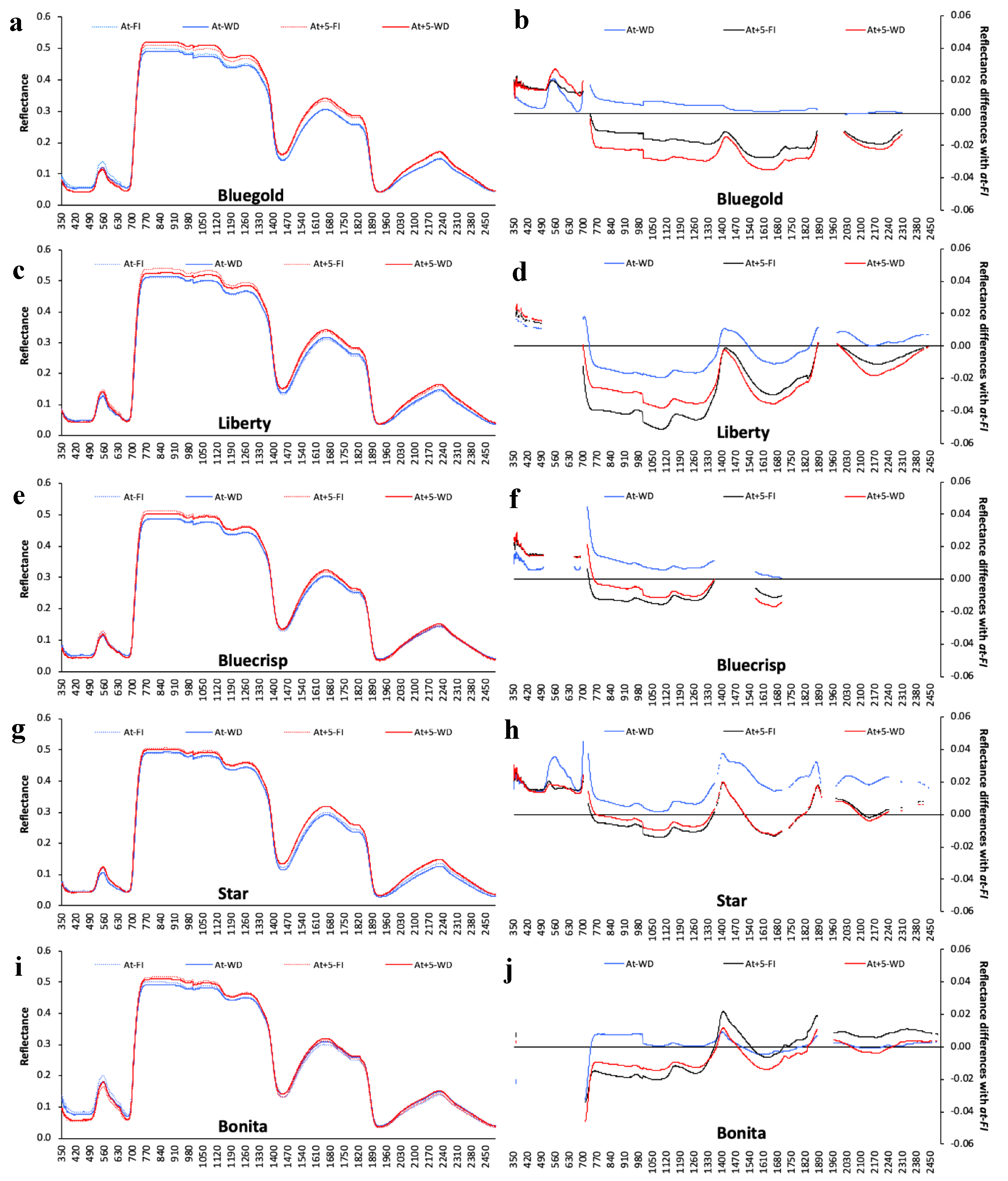
3.5. Determining the Environmental Effects in the Leaf Spectral Signature

When the spectral signatures of each genotype were compared (Figure 5a,c,e,g,i; Table S3), differences between environments were clearer in those blueberries growing with and without heat stress (red and blue lines, respectively); dissimilarities were more consistent from ~740 nm onwards. Within each heat condition, differences between environments were difficult to examine. On the other hand, the proposed methodology to contrast the control spectral signature (at–FI) with the characteristic reflectance under each adverse condition (at–WD, at₊₅–FI and at₊₅–WD) allowed the magnification of the differences between the compared reflections (Figure 5b,d,f,h,j). In terms of magnitude, a greater number of differences were observed with at₊₅–FI (black lines) and at₊₅–WD (red lines) than in an environment without heat stress (at–WD; blue lines) (Figure 5b,d,f,h,j).

When the averaged reflectances under the adverse conditions were compared with that of the control (Figure 5b,d,f,h,j), a larger range of differences were observed, recognizing four comparable stretches: i) ~350–710 nm: V. ashei ‘Bonita’ (Figure 5j) behaved differently to V. corymbosum cultivars (Figure 5b,d,f,h); V. corymbosum was more reflective than the control, whereas V. ashei showed no differences between environments; ii) ~710–1450 nm: before the peak at 1450 nm, the responses varied according to the treatment and cultivar; this was the only section where all the cultivars proved to respond differently among the conditions studied. In general, the differences between at₊₅–FI and at₊₅–WD were minor in the southern V. corymbosum ‘Bluecrisp’ and ‘Star’ (Figure 5f,h) and V. ashei ‘Bonita’ (Figure 5j), but larger in the northern V. corymbosum ‘Bluegold’ and ‘Liberty’ (Figure 5b,d). In relation to at–WD, due to it lesser distance from the at–FI, the northern V. corymbosum ‘Bluegold’ (Figure 5b) and V. ashei ‘Bonita’ (Figure 5j; blue line) appeared to be less influenced by water deficit than the rest of the cultivars; iii) ~1450–1880 nm: the spectral signatures differed in a small region common to all cultivars, plateau between both extremes (~1570–1700 nm), in which a greater number of different patterns between environments was observed. The southern V. corymbosum ‘Star’ (Figure 5h) was notable because it showed the largest differences between at–FI and at–WD, and when heat stress was present its spectral signatures were not influenced by the water content in the pots (at₊₅–FI and at₊₅–WD; black and red lines); and iv) ~1880–2500 nm: in the significant common section (2100–2250 nm), the ‘Star’ cultivar (Figure 5h) under at–WD differed the most from the control, and when heat stress was present, the spectral signatures of at₊₅–FI and at₊₅–WD were relatively similar. Additionally, V. corymbosum ‘Bluegold’ (Figure 5b) and V. ashei ‘Bonita’ (Figure 5j) seemed to be less influenced than the rest of the cultivars when they were grown under at–WD.

4. Discussion

The incorporation of physiological assessments in plant breeding programs will become increasingly important, not only for the estimation of specific traits, but also for the simultaneous integration of a number of different characters, improving the chances of identifying cultivars well-adapted to the more challenging environments predicted for the future [3,4].

Studies in which physiological traits have been estimated by spectral reflectance are varied in terms of equipment used (e.g., manufacturer, resolution and spectral sample, reproducibility and accuracy), methodology of reflectance measurements (e.g., calibration procedure, distance to the measured object, use and intensity of light source, angle of measurement, screening of a single spot or moving the fiber across the plot, number of scans per plot, and integration time), and data analysis (e.g., the criterion of elimination of spectral noise, with or without prior wavelength selection, and linear and nonlinear approximations). Therefore, not only it is difficult to compare results between studies but, due to the same reasons, it is also inadequate on many occasions.

Methodologically, the first point of interest is the modeling criterion when the environmental conditions were evaluated together (All); usually performed better when higher coefficients of determination are looked for by the increment of the trait-range [20]. Interestingly, the results of the present study suggest that blueberry models, in general, had a better performance when the environments were considered separately, at least when a proximal approach (leaf clip with light source) is used. When [17] and [20] estimated several physiological and productive traits by non-proximal spectral reflectance (80 cm above the canopy); it was concluded that the estimations were always improved when data from the contrasting water supply conditions (fully irrigated, mild and severe water deficit) were combined.

In most instances (i.e., variables, environments, wavelength selection criterion, and modeling methodology), PLS was superior to MLR. In this regard, the PLS method transforms the space of spectral properties so that the resulting factors represent the maximum variation in the covariance of the variable being evaluated. This produces efficient data compression and therefore a better calibration model compared to other linear statistical methods [48,49,50]. Furthermore, the PLS method is based on a projection of the predictors (x) and response (y) variables into a set of latent variables (or PLS factors) and corresponding scores, minimizing the dimensionality of the data while maximizing the covariance between x and y variables [27].

On the other hand, as expected, MLR W/O was not a suitable methodology for modeling spectral data. It was common that a prior wavelength selection, especially MC, did improve the estimation (R²_Val values) of the different variables analyzed (Figure 1, Figure 2, Figure 3 and Figure 4, and Table S2). Although the MLR R²_Val values were lower than the PLS, there are studies where a previous selection of wavelengths improved the predictive ability of MLR over PLS, or at least both methodologies were of equal strength [30,40,41].

The variables analyzed in this study are considered key for physiological breeding approaches [51], many of which have not previously been modeled by the use of spectral reflectance, especially in fruit breeding programs [3,4]. Among the characters delivering valuable information about plant physiological status, photosynthetic pigments are probably the most extensively studied, especially the chlorophylls, where a strong association with the nitrogen content has been described [10,52,53]. Independent of the plant species studied or the modeling methodology utilized for predicting chlorophyll concentration (Chl a, Chl b or Chl total), the coefficients of determination reported in the literature are usually high (R²_Val > 0.65) [10,41,48,54,55], which is coincident with the results presented in this work. Interestingly, the higher R²_Val values that were obtained for the estimation of Chl a/b values are also superior to those documented by other authors, which have been generated either via predictive models or through the study of SRIs [56]. The chlorophyll a and b ratio (Chl a/b) is a good indicator of stress in higher plants [57,58]. Stress conditions generate oxidative damage, causing a decrease in the chlorophyll content due to degradation of chlorophylls, deficiency in chlorophyll synthesis, and also because of changes in the thylakoid membrane structure [59]. Low values of Chl a/b in leaves under drought conditions are caused by higher Chl a degradation rates compared to Chl b due to the conversion of Chl a to Chl b by the oxidation of the methyl group on ring II to an aldehyde group [60,61]. In this sense, using the same individuals assessed in the current study, [47] proved that Chl a/b was relevant in identifying blueberry genotypes subjected to heat stress.

Due to the time involved in screening plant water status via pressure chambers, there has been significant effort invested in estimating SWP by remote sensing technologies [19]. In this study, the R²_Val values of the SWP under individual environmental conditions were, in general, lower than those found in other species such as olives (R²_Val ~0.7) [19,62] or grapevines (0.71 < R²_Val < 0.84) [63,64,65]. In general, most of the published studies combine more than one environmental condition, generating higher R²_Val because of the forced dispersal of the data cloud along the x-axis [20], which would explain the lower R²_Val values in this study. In addition, correlations could be influenced by the particular blueberry root morphology and physiology; shallow fibrous roots, which are also very thin and without root hairs, responding differently to the hydric deficit [66,67].

The prediction of leaf gas exchange variables using spectral data has been less studied. Most of the literature has focused on relating some SRIs, usually the photochemical reflectance index (PRI), with the state or activity of the photosynthetic apparatus [68,69,70,71]. The results of the present study are similar to those found by [15] using the same proximal approach in wheat leaves, reporting R²_Val for A and gs of 0.34 and 0.49, respectively. In olives, [17] described higher coefficients of determination at the branch level for A (R²_Val = 0.81), gs (R²_Val = 0.78) and E (R²_Val = 0.81); however, the wide range of SWP generated by olive trees under drought conditions could have influenced the higher coefficients of determination. Indeed, the study of water availability in olive orchards generated a broader range of potentials (−1.7 to −6.2 MPa) [72] than those reported by [47] using the same blueberry individuals considered in the present study (−0.2 to −2.5 MPa).

In parallel with leaf gas exchange, several studies have attempted to estimate some chlorophyll a fluorescence parameters using SRIs [73,74,75,76,77]; however, multivariate regression analyses of the spectral signatures have not been described in the literature. The parameters derived from rapid light curves are important for breeders because they would allow recognition of genotype behavior such as the rate of electrons passing from PSII to PSI, the amount of light saturating the photosystems, and the efficiency of electrons reaching the light-harvesting antenna for use in photosynthesis [78,79]. In this regard, genotypes having high values of ETR_max, Alpha and IK should have a better photosynthetic performance under stress conditions [47,80,81]. When drought or elevated temperatures are present, the photoprotective capacity in leaves decreases and photo-oxidative damage of PSII occurs with irreversible losses of reaction centers [82,83,84]. The results shown in the current work are relevant because some of the most important parameters (ETR_max and IK), previously reported as being key for discriminating between blueberry genotypes growing under water deficit conditions [47], were estimated with relatively high coefficients of determination (ETR_max ≤ 0.60 and IK ≤ 0.59).

The classical comparison of the spectral signatures in each one of the four environments (Figure 5a,c,e,g,i) did not identify substantial differences between environmental scenarios. A different approach to characterize and interpret the environmental effects on the evaluated genotypes is to analyze changes at the spectral signature level. As was previously mentioned, the spectral signature is closely associated with the absorption of certain wavelengths, linked to specific characteristics or plant conditions [8,9,10,11]. Consequently, the environmental differences that a genotype undergoes should be translated into modifications at the reflectance level too.

When the averaged reflectances under the adverse conditions (at–WD, at₊₅–FI and at₊₅–WD) were compared with that of the control (at–FI) (Figure 5), cultivars varied in their responses according to the studied stress (drought, heat, or both). Besides the fact that there is variation in leaf anatomy and cell structure between genotypes [3,17], differences within the same species (V. corymbosum) were expected because blueberry breeders have incorporated genes from many species within the Vaccinium genus through inter-specific hybridization [3]. For example, ‘Liberty’ (northern V. corymbosum) is 100 %V. corymbosum while ‘Star’ (southern V. corymbosum) is estimated to genetically comprise 78, 8, 7, 2, and 1% V. corymbosum, V. angustifolium, V. darrowii, V. ashei, and V. tenellum, respectively. This inter-specific hybridization confers useful characteristics to overcome environmental constraints. For example, V. darrowii and V. ashei have been identified as species having a higher level of heat and drought tolerance, respectively; both species were initially collected from the South East of North America [85]. Since both southern highbush ‘Bluecrisp‘ and ‘Star‘ have a proportion of V. darrowii in their pedigree, it would be possible to hypothesize that the smaller distances between the overheated environments (at₊₅–FI and at₊₅–WD), comparison lines (black and red in Figure 5f,h), could be due to a greater heat tolerance. Rabbiteye (V. ashei) ‘Bonita’, from ~740 nm onwards, presented almost no differences from the control treatment, probably also associated with the drought tolerance characteristics of this species; if this is true, it would mean that, in the case of ‘Bluegold‘, the similarity of the spectral signatures of at–FI and at–WD (blue line in Figure 5b) could be due to a greater capacity to tolerate a lack of water. These preliminary results would indicate that the presented methodology (changes relative to the control), could be considered for the identification of tolerant/susceptible genotypes for a specific environmental condition.

5. Conclusions and Future Perspectives

In general, PLS showed better results than MLR, regardless of the methodology used in the selection of the wavelengths. Considering the low predictive values of MLR, with few exceptions, there was an increase in trait estimation (R²_Val) using MC over GA for predictor selection. Chl a/b, ETR_max and IK were among the variables with the highest coefficients of determination of validation, which contrasted with the poor estimations reached for Alpha, qP, qN and Y(II). The results of this study reaffirm that, by the modeling of the spectral reflectance, it is possible to assess some key traits (e.g., Chl a/b, ETR_max and IK) that could begin to be used in blueberry breeding programs oriented to adaptation to the new challenging environmental scenarios.

Even if it could be argued that it is disadvantageous to work with potted plants under controlled environments and reflectance assessed by a proximal approach, as performed by other authors in maize and wheat (Yendrek et al., 2017; Silva-Perez et al., 2018) [15,86], there are still some important advantages to highlight: (i) the minimum spectral noise compared to a non-proximal measurement helps to identify the potential of this technology in fruit breeding programs; (ii) under field conditions, it is difficult to study spectral signature changes of isolated and combined environmental conditions (drought and heat); (iii) in the case commercial blueberry production, an important part of the southern highbush cultivars are grown in pots with peat moss and in greenhouses [87,88], primarily subjected to high temperature conditions, so breeders are also programming crosses for these type of environments; and (iv) assessments are considerably faster than the classic eco-physiological measurements, allowing the screening of a much higher number of genotypes in a short period of time [15,86]. The selected genotypes can then be tested in more sophisticated field trials as part of the advanced variety selection [4,89].

For increasing measurement speed and to allow integration of a larger proportion of the canopy, future efforts should consider a non-proximal approach. To the extent that the use of phenomics is of major relevance and a greater number of seasons are available for modeling, the implementation of a completely independent validation of calibration models should be undertaken. As proposed by [20], a multivariate classification modeling approximation (e.g., PLS-DA) should also improve the predictive capacity, at least for the group of elite genotypes.

The preliminary results from the study of the spectral signature with respect to the control treatment could represent an easier and more direct way to evaluate the tolerance or susceptibility to a specific environmental condition. In this sense, continuous measurements of the spectral signature through periods of adverse conditions could help us gain better identification and hence understanding of the wavelengths involved and the magnitudes associated with the particular condition.

References

1. Moretti, C.L.; Mattos, L.M.; Calbo, A.G.; Sargent, S.A. Climate changes and potential impacts on postharvest quality of fruit and vegetable crops: A review. Food Res. Int. 2010, 43, 1824–1832. [Google Scholar] [CrossRef]
2. Osborne, T.; Rose, G.; Wheeler, T. Variation in the global-scale impacts of climate change on crop productivity due to climate model uncertainty and adaptation. Agric. For. Meteorol. 2013, 170, 183–194. [Google Scholar] [CrossRef]
3. Lobos, G.A.; Hancock, J.F. Breeding blueberries for a changing global environment: A review. Front. Plant Sci. 2015, 6. [Google Scholar] [CrossRef] [PubMed]
4. Camargo, A.; Lobos, G.A. Latin America: A development pole for phenomics. Front. Plant Sci. 2016, 7. [Google Scholar] [CrossRef]
5. Passioura, J.B. Phenotyping for drought tolerance in grain crops: When is it useful to breeders? Funct. Plant Biol. 2012, 39, 851–859. [Google Scholar] [CrossRef]
6. Araus, J.L.; Elazab, A.; Vergara, O.; Cabrera-Bosquet, L.; Serret, M.D.; Zaman-Allah, M.; Cairns, J.E. New technologies for phenotyping. In Phenomics: How Next-Generation Phenotyping Is Revolutionizing Plant Breeding; Fritsche-Neto, R., Borém, A., Eds.; Springer: New York, NY, USA, 2015; pp. 1–14. [Google Scholar]
7. Houle, D.; Govindaraju, D.R.; Omholt, S. Phenomics: The next challenge. Nat. Rev. Genet. 2010, 11, 855–866. [Google Scholar] [CrossRef] [PubMed]
8. Garbulsky, M.F.; Peñuelas, J.; Gamon, J.; Inoue, Y.; Filella, I. The photochemical reflectance index (PRI) and the remote sensing of leaf, canopy and ecosystem radiation use efficiencies: A review and meta-analysis. Remote Sens. Environ. 2011, 115, 281–297. [Google Scholar] [CrossRef]
9. Araus, J.L.; Cairns, J.E. Field high-throughput phenotyping: the new crop breeding frontier. Trends Plant Sci. 2014, 19, 52–61. [Google Scholar] [CrossRef] [PubMed]
10. Garriga, M.; Retamales, J.B.; Romero-Bravo, S.; Caligari, P.D.; Lobos, G.A. Chlorophyll, anthocyanin, and gas exchange changes assessed by spectroradiometry in Fragaria chiloensis under salt stress. J. Integr. Plant Biol. 2014, 56, 505–515. [Google Scholar] [CrossRef]
11. Hernandez, J.; Lobos, G.A.; Matus, I.; del Pozo, A.; Silva, P.; Galleguillos, M. Using ridge regression models to estimate grain yield from field spectral data in bread wheat (Triticum aestivum L.) grown under three water regimes. Remote Sens. 2015, 7, 2109–2126. [Google Scholar] [CrossRef]
12. Lopes, M.S.; Araus, J.L.; Van Heerden, P.D.R.; Foyer, C.H. Enhancing drought tolerance in C4 crops. J. Exp. Bot. 2011, 62, 3135–3153. [Google Scholar] [CrossRef] [Green Version]
13. Prasanna, B.M.; Araus, J.L.; Crossa, J.; Cairns, J.E.; Palacios, N.; Mahuku, G.; Das, B.; Magorokosho, C. High-throughput and precision phenotyping in cereal breeding programs. In Cereal Genomics-II; Gupta, P.K., Varshney, R.K., Eds.; Springer: Dordrecht, The Netherlands, 2012; pp. 341–374. [Google Scholar]
14. Cabrera-Bosquet, L.; Crossa, J.; von Zitzewitz, J.; Serret, M.D.; Araus, J.L. High-throughput phenotyping and genomic selection: The frontiers of crop breeding converge. J. Integr. Plant Biol. 2012, 54, 312–320. [Google Scholar] [CrossRef] [PubMed]
15. Silva-Perez, V.; Molero, G.; Serbin, S.P.; Condon, A.G.; Reynolds, M.P.; Furbank, R.T.; Evans, J.R. Hyperspectral reflectance as a tool to measure biochemical and physiological traits in wheat. J. Exp. Bot. 2018, 69, 483–496. [Google Scholar] [CrossRef] [PubMed]
16. Lobos, G.A.; Poblete-Echeverría, C.; Ahumada, L.; Zúñiga, M.; Romero, S.; Escobar, A.; Caligari, P.D.S. Fast and non-destructive prediction of gas exchange in olive orchards (Olea europaea L.) under different soil water conditions. Acta Hortic. 2014, 1057, 329–334. [Google Scholar] [CrossRef]
17. Lobos, G.A.; Matus, I.; Rodriguez, A.; Romero-Bravo, S.; Araus, J.L.; del Pozo, A. Wheat genotypic variability in grain yield and carbon isotope discrimination under Mediterranean conditions assessed by spectral reflectance. J. Integr. Plant Biol. 2014, 56, 470–479. [Google Scholar] [CrossRef] [PubMed] [Green Version]
18. Poblete-Echeverría, C.; Ortega-Farías, S.; Lobos, G.A.; Romero, S.; Ahumada, L.; Escobar, A.; Fuentes, S. Non-invasive method to monitor plant water potential of an olive orchard using visible and near infrared spectroscopy analysis. Acta Hortic. 2014, 1057, 363–368. [Google Scholar] [CrossRef]
19. Lobos, G.A.; Poblete-Echeverría, C. Spectral Knowledge (SK-UTALCA): Software for exploratory analysis of high-resolution spectral reflectance data on plant breeding. Front. Plant Sci. 2017, 7. [Google Scholar] [CrossRef] [PubMed]
20. Garriga, M.; Romero-Bravo, S.; Estrada, F.; Escobar, A.; Matus, I.A.; del Pozo, A.; Astudillo, C.A.; Lobos, G.A. Assessing wheat traits by spectral reflectance: Do we really need to focus on predicted trait-values or directly identify the elite genotypes group? Front. Plant Sci. 2017, 8, 280. [Google Scholar] [CrossRef]
21. Leardi, R.; Seasholtz, M.B.; Pell, R.J. Variable selection for multivariate calibration using a genetic algorithm: prediction of additive concentrations in polymer films from Fourier transform-infrared spectral data. Anal. Chim. Acta-Comp. 2002, 461, 189–200. [Google Scholar] [CrossRef]
22. Thenkabail, P.S.; Smith, R.B.; De Pauw, E. Hyperspectral vegetation indices and their relationships with agricultural crop characteristics. Remote Sens. Environ. 2000, 71, 158–182. [Google Scholar] [CrossRef]
23. Nguyen, H.T.; Lee, B.W. Assessment of rice leaf growth and nitrogen status by hyperspectral canopy reflectance and partial least square regression. Eur. J. Agron. 2006, 24, 349–356. [Google Scholar] [CrossRef]
24. Hurvich, C.M.; Tsai, C.L. Regression and time series model selection in small samples. Biometrika 1989, 76, 297–307. [Google Scholar] [CrossRef]
25. Hawkins, D. The problem of overfitting. J. Chem. Inf. Comput. Sci. 1990, 44, 1–12. [Google Scholar] [CrossRef] [PubMed]
26. Norgaard, L.; Saudland, J.; Wagner, J.; Nielsen, J.P.; Munck, L.; Engelsen, S.B. Interval partial least-squares regression (iPLS): A comparative chemometric study with an example from near-infrared spectroscopy. Appl. Spectrosc. 2000, 54, 413–419. [Google Scholar] [CrossRef]
27. Wold, S.; Sjöström, M.; Eriksson, L. PLS-regression: A basic tool of chemometrics. Chemometr. Intell. Lab. 2001, 58, 109–130. [Google Scholar] [CrossRef]
28. Balabin, R.M.; Safieva, R.Z.; Lomakina, E.I. Comparison of linear and nonlinear calibration models based on near infrared (NIR) spectroscopy data for gasoline properties prediction. Chemometr. Intell. Lab. 2007, 88, 183–188. [Google Scholar] [CrossRef]
29. Næs, T.; Mevik, B.H. Understanding the collinearity problem in regression and discriminant analysis. J. Chemom. 2001, 15, 413–426. [Google Scholar] [CrossRef]
30. Wu, D.; Chen, J.; Lu, B.; Xiong, L.; He, Y.; Zhang, Y. Application of near infrared spectroscopy for the rapid determination of antioxidant activity of bamboo leaf extract. Food Chem. 2012, 135, 2147–2156. [Google Scholar] [CrossRef] [PubMed]
31. Jouan-Rimbaud, D.; Massart, D.L.; Leardi, R.; De Noord, O.E. Genetic algorithms as a tool for wavelength selection in multivariate calibration. Anal. Chem. 1995, 67, 4295–4301. [Google Scholar] [CrossRef]
32. Leardi, R. Application of genetic algorithm-PLS for feature selection in spectral data sets. J. Chemom. 2000, 14, 643–655. [Google Scholar] [CrossRef]
33. Leardi, R.; Norgaard, L. Sequential application of backward interval partial least squares and genetic algorithms for the selection of relevant spectral regions. J. Chemom. 2004, 18, 486–497. [Google Scholar] [CrossRef]
34. Li, L.; Ustin, S.L.; Riano, D. Retrieval of fresh leaf fuel moisture content using genetic algorithm partial least squares (GA-PLS) modeling. IEEE Geosci. Remote Sens. Lett. 2007, 4, 216–220. [Google Scholar] [CrossRef]
35. Arakawa, M.; Yamashita, Y.; Funatsu, K. Genetic algorithm-based wavelength selection method for spectral calibration. J. Chemometr. 2011, 25, 10–19. [Google Scholar] [CrossRef]
36. Sratthaphut, L.; Ruangwises, N. Genetic algorithms-based approach for wavelength selection in spectrophotometric determination of vitamin B12 in pharmaceutical tablets by partial least-squares. Procedia Eng. 2012, 32, 225–231. [Google Scholar] [CrossRef]
37. Givianrad, M.H.; Saber-Tehrani, M.; Zarin, S. Genetic algorithm-based wavelength selection in multicomponent spectrophotometric determinations by partial least square regression: Application to a sulfamethoxazole and trimethoprim mixture in bovine milk. J. Serb. Chem. Soc. 2013, 78, 555–564. [Google Scholar] [CrossRef]
38. Goldberg, D.E.; Holland, J.H. Genetic algorithms and machine learning. Mach. Learn. 1988, 3, 95–99. [Google Scholar] [CrossRef]
39. Goicoechea, H.C.; Olivieri, A.C. Wavelength selection for multivariate calibration using a genetic algorithm: A novel initialization strategy. J. Chem. Inf. Comp. Sci. 2002, 42, 1146–1153. [Google Scholar] [CrossRef]
40. Li, Z.; Wang, J.; Xiong, Y.; Li, Z.; Feng, S. The determination of the fatty acid content of sea buckthorn seed oil using near infrared spectroscopy and variable selection methods for multivariate calibration. Vib. Spectrosc. 2016, 84, 24–29. [Google Scholar] [CrossRef]
41. Zhang, J.; Liu, J.; Yang, C.; Du, S.; Yang, W. Photosynthetic performance of soybean plants to water deficit under high and low light intensity. S. Afr. J. Bot. 2016, 105, 279–287. [Google Scholar] [CrossRef]
42. Fang, M.; Li, H.; Liu, Z.; Xian, X. Online evaluation of yellow peach quality by visible and near-infrared spectroscopy. Adv. J. Food Sci. Technol. 2013, 5, 606–612. [Google Scholar] [CrossRef]
43. Bryla, D.R.; Strik, B.C. Effects of cultivar and plant spacing on the seasonal water requirements of highbush blueberry. J. Am. Soc. Hortic. Sci. 2007, 132, 270–277. [Google Scholar] [CrossRef]
44. Lobos, G.A.; Retamales, J.B.; Hancock, J.F.; Flore, J.A.; Cobo, N.G.; del Pozo, A. Spectral irradiance, gas exchange characteristics and leaf traits of Vaccinium corymbosum L. ‘Elliott’ grown under photo-selective nets. Environ. Exp. Bot. 2012, 75, 142–149. [Google Scholar] [CrossRef]
45. Moran, R.; Porath, D. Chlorophyll determination in intact tissues using N,N-dimethylformamide. Plant Physiol. 1980, 65, 478–479. [Google Scholar] [CrossRef] [PubMed]
46. Inskeep, W.P.; Bloom, P.R. Extinction coefficients of chlorophyll a and b in N,N-dimethylformamide and 80% acetone. Plant Physiol. 1985, 77, 483–485. [Google Scholar] [CrossRef] [PubMed]
47. Estrada, F.; Escobar, A.; Romero-Bravo, S.; González-Talice, J.; Poblete-Echeverría, C.; Caligari, P.D.; Lobos, G.A. Fluorescence phenotyping in blueberry breeding for genotype selection under drought conditions, with or without heat stress. Sci. Hortic. 2015, 181, 147–161. [Google Scholar] [CrossRef]
48. Atzberger, C.; Guérif, M.; Baret, F.; Werner, W. Comparative analysis of three chemometric techniques for the spectroradiometric assessment of canopy chlorophyll content in winter wheat. Comput. Electron. Agric. 2010, 73, 165–173. [Google Scholar] [CrossRef]
49. Herrmann, I.; Pimstein, A.; Karnieli, A.; Cohen, Y.; Alchanatis, V.; Bonfil, D.J. LAI assessment of wheat and potato crops by VENUS and Sentinel-2 bands. Remote Sens. Environ. 2011, 115, 2141–2151. [Google Scholar] [CrossRef]
50. Gredilla, A.; de Vallejuelo, S.F.O.; Elejoste, N.; de Diego, A.; Madariaga, J.M. Non-destructive spectroscopy combined with chemometrics as a tool for green chemical analysis of environmental samples: A review. Trends Anal. Chem. 2016, 76, 30–39. [Google Scholar] [CrossRef]
51. Reynolds, M.; Langridge, P. Physiological breeding. Curr. Opin. Plant. Biol. 2016, 31, 162–171. [Google Scholar] [CrossRef] [Green Version]
52. Gitelson, A.A.; Merzlyak, M.N. Non-destructive assessment of chlorophyll carotenoid and anthocyanin content in higher plant leaves: principles and algorithms. Pap. Nat. Resour. 2004, 263, 78–94. [Google Scholar]
53. Vergara-Díaz, O.; Zaman-Allah, M.A.; Masuka, B.; Hornero, A.; Zarco-Tejada, P.; Prasanna, B.M.; Araus, J.L. A novel remote sensing approach for prediction of maize yield under different conditions of nitrogen fertilization. Front. Plant Sci. 2016, 7. [Google Scholar] [CrossRef] [PubMed]
54. Tumbo, S.D.; Wagner, D.G.; Heinemann, P.H. Hyperspectral based neural network for predicting chlorophyll status in corn. Trans. ASABE 2002, 45, 825–832. [Google Scholar] [CrossRef]
55. Doughty, C.E.; Asner, G.P.; Martin, R.E. Predicting tropical plant physiology from leaf and canopy spectroscopy. Oecologia 2011, 165, 289–299. [Google Scholar] [CrossRef]
56. Nyongesah, M.J.; Wang, Q.; Li, P. Effectiveness of photochemical reflectance index to trace vertical and seasonal chlorophyll a/b ratio in Haloxylon ammodendron. Acta Physiol. Plant. 2015, 37, 1–11. [Google Scholar] [CrossRef]
57. Camejo, D.; Rodríguez, P.; Morales, M.A.; Dell’Amico, J.M.; Torrecillas, A.; Alarcón, J.J. High temperature effects on photosynthetic activity of two tomato cultivars with different heat susceptibility. J. Plant. Physiol. 2005, 162, 281–289. [Google Scholar] [CrossRef] [PubMed]
58. Bacelar, E.A.; Santos, D.L.; Moutinho-Pereira, J.M.; Lopes, J.I.; Gonçalves, B.C.; Ferreira, T.C.; Correia, C.M. Physiological behaviour, oxidative damage and antioxidative protection of olive trees grown under different irrigation regimes. Plant Soil 2007, 292, 1–12. [Google Scholar] [CrossRef]
59. Smirnoff, N. The role of active oxygen in the response of plants to water deficit and desiccation. New Phytol. 1993, 125, 27–58. [Google Scholar] [CrossRef]
60. Fang, Z.; Bouwkamp, J.C.; Solomos, T. Chlorophyllase activities and chlorophyll degradation during leaf senescence in non-yellowing mutant and wild type of Phaseolus vulgaris L. J. Exp. Bot. 1998, 49, 503–510. [Google Scholar] [CrossRef]
61. Evans, J.R. Photosynthetic acclimation and nitrogen partitioning within a lucerne canopy. I Canopy characteristics. Aust. J. Plant. Physiol. 1993, 20, 55–67. [Google Scholar] [CrossRef]
62. Gutiérrez, S.; Tardaguila, J.; Fernández-Novales, J.; Diago, M.P. Data mining and NIR spectroscopy in viticulture: Applications for plant phenotyping under field conditions. Sensors 2016, 16, 236. [Google Scholar] [CrossRef]
63. Santos, A.O.; Kaye, O. Grapevine leaf water potential based upon near infrared spectroscopy. Sci. Agric. 2009, 66, 287–292. [Google Scholar] [CrossRef] [Green Version]
64. De Bei, R.; Cozzolino, D.; Sullivan, W.; Cynkar, W.; Fuentes, S.; Dambergs, R.; Tyerman, S. Non-destructive measurement of grapevine water potential using near infrared spectroscopy. Aust. J. Grape Wine R. 2011, 17, 62–71. [Google Scholar] [CrossRef]
65. Vila, H.; Hugalde, I.; Di Filippo, M. Estimación de potencial hídrico en vid por medio de medidas termográficas y espectrales. Rev. Inv. Agropec. 2011, 37, 46–52. [Google Scholar]
66. Valenzuela-Estrada, L.R.; Vera-Caraballo, V.; Ruth, L.E.; Eissenstat, D.M. Root anatomy, morphology, and longevity among root orders in Vaccinium corymbosum (Ericaceae). Am. J. Bot. 2008, 95, 1506–1514. [Google Scholar] [CrossRef]
67. Valenzuela-Estrada, L.R.; Richards, J.H.; Diaz, A.; Eissensat, D.M. Patterns of nocturnal rehydration in root tissues of Vaccinium corymbosum L. under severe drought conditions. J. Exp. Bot. 2009, 60, 1241–1247. [Google Scholar] [CrossRef] [PubMed]
68. Marino, G.; Pallozzi, E.; Cocozza, C.; Tognetti, R.; Giovannelli, A.; Cantini, C.; Centritto, M. Assessing gas exchange, sap flow and water relations using tree canopy spectral reflectance indices in irrigated and rainfed Olea europaea L. Environ. Exp. Bot. 2014, 99, 43–52. [Google Scholar] [CrossRef]
69. Tsonev, T.; Wahbi, S.; Sun, P.; Sorrentino, G.; Centritto, M. Gas exchange, water relations and their relationships with photochemical reflectance index in Quercus ilex plants during water stress and recovery. Int. J. Agric. Biol. 2014, 16, 335–341. [Google Scholar]
70. Fréchette, E.; Wong, C.Y.; Junker, L.V.; Chang, C.Y.Y.; Ensminger, I. Zeaxanthin-independent energy quenching and alternative electron sinks cause a decoupling of the relationship between the photochemical reflectance index (PRI) and photosynthesis in an evergreen conifer during spring. J. Exp. Bot. 2015, 66, 7309–7323. [Google Scholar] [CrossRef] [Green Version]
71. Fréchette, E.; Chang, C.Y.Y.; Ensminger, I. Photoperiod and temperature constraints on the relationship between the photochemical reflectance index and the light use efficiency of photosynthesis in Pinus strobus. Tree Physiol. 2016, 36, 311–324. [Google Scholar] [CrossRef]
72. Poblete-Echeverría, C.; Sepulveda-Reyes, D.; Ortega-Farias, S.; Zuñiga, M.; Fuentes, S. Plant water stress detection based on aerial and terrestrial infrared thermography: A study case from vineyard and olive orchard. Acta Hortic. 2016, 1112, 141–146. [Google Scholar] [CrossRef]
73. Zarco-Tejada, P.J.; Miller, J.R.; Mohammed, G.H.; Noland, T.L. Chlorophyll fluorescence effects on vegetation apparent reflectance: I. Leaf-level measurements and model simulation. Remote Sens. Environ. 2000, 74, 582–595. [Google Scholar] [CrossRef]
74. Zarco-Tejada, P.; Miller, J.; Mohammed, G.; Noland, T.; Sampson, P. Estimation of chlorophyll fluorescence under natural illumination from hyperspectral data. Int. J. Appl. Earth Obs. 2001, 3, 321–327. [Google Scholar] [CrossRef] [Green Version]
75. Zarco-Tejada, P.; Pushnik, J.C.; Dobrowski, S.; Ustin, S.L. Steady-state chlorophyll a fluorescence detection from canopy derivative reflectance and double-peak red-edge effects. Remote Sens. Environ. 2003, 84, 283–294. [Google Scholar] [CrossRef]
76. Meroni, M.; Rossini, M.; Picchi, V.; Panigada, C.; Cogliati, S.; Nali, C.; Colombo, R. Assessing steady-state fluorescence and PRI from hyperspectral proximal sensing as early indicators of plant stress: The case of ozone exposure. Sensors 2008, 8, 1740–1754. [Google Scholar] [CrossRef] [PubMed]
77. Zhang, H.; Zhua, L.; Hu, H.; Zhen, K.; Jina, Q. Monitoring leaf chlorophyll fluorescence with spectral reflectance in rice (Oryza sativa L.). Procedia Eng. 2011, 15, 4403–4408. [Google Scholar] [CrossRef]
78. Ralph, P.J.; Gademann, R. Rapid light curves: A powerful tool to assess photosynthetic activity. Aquat. Bot. 2005, 82, 222–237. [Google Scholar] [CrossRef]
79. Klughammer, C.; Schreiber, U. Complementary PS II quantum yields calculated from simple fluorescence parameters measured by PAM fluorometry and the saturation pulse method. PAM Appl. Notes 2008, 1, 27–35. [Google Scholar]
80. Deeba, F.; Pandey, A.K.; Ranjan, S.; Mishra, A.; Singh, R.; Sharma, Y.K.; Pandey, V. Physiological and proteomic responses of cotton (Gossypium herbaceum L.) to drought stress. Plant Physiol. Biochem. 2012, 53, 6–18. [Google Scholar] [CrossRef]
81. Lideman, L.; Nishihara, G.N.; Noro, T.; Terada, R. Effect of temperature and light on the photosynthesis as measured by chlorophyll fluorescence of cultured Eucheuma denticulatum and Kappaphycus sp. (Sumba strain) from Indonesia. J. Appl. Phycol. 2013, 25, 399–406. [Google Scholar] [CrossRef]
82. Percival, D.C.; Sharpe, S.; Maqbool, R.; Zaman, Q. Narrow band reflectance measurements can be used to estimate leaf area index, flower number, fruit set and berry yield of the wild blueberry (Vaccinium angustifolium Ait.). Acta Hortic. 2012, 926, 363–369. [Google Scholar] [CrossRef]
83. Glass, V.M.; Percival, D.C.; Proctor, J.T.A. Tolerance of lowbush blueberries (Vaccinium angustifolium Ait.) to drought stress. I. Soil water and yield component analysis. Can. J. Plant Sci. 2005, 85, 911–917. [Google Scholar] [CrossRef]
84. Rho, H.; Yu, D.J.; Kim, S.J.; Lee, H.J. Limitation factors for photosynthesis in ‘Bluecrop’ highbush blueberry (Vaccinium corymbosum) leaves in response to moderate water stress. J. Plant Biol. 2012, 55, 450–457. [Google Scholar] [CrossRef]
85. Hancock, J.F.; Lyrene, P.; Finn, C.E.; Vorsa, N.; Lobos, G.A. Blueberry and cranberry. In Temperate Fruit Crop Breeding: Germplasm to Genomics; Hancock, J.F., Ed.; Kluwer Academic Publishers: Dordrecht, The Netherlands, 2008; pp. 115–149. [Google Scholar]
86. Yendrek, C.R.; Tomaz, T.; Montes, C.M.; Cao, Y.; Morse, A.M.; Brown, P.J.; McIntyre, L.M.; Leakey, A.D.B.; Ainsworth, E.A. High-throughput phenotyping of maize leaf physiological and biochemical traits using hyperspectral reflectance. Plant Physiol. 2017, 173, 614. [Google Scholar] [CrossRef] [PubMed]
87. Voogt, W.; van Dijk, P.; Douven, F.; van der Maas, R. Development of a soilless growing system for blueberries (Vaccinium corymbosum): Nutrient demand and nutrient solution. Acta Hortic. 2014, 1017, 215–221. [Google Scholar] [CrossRef]
88. Kingston, P.H.; Scagel, C.F.; Bryla, D.R.; Strik, B. Suitability of sphagnum moss, coir, and douglas fir bark as soilless substrates for container production of highbush blueberry. HortScience 2017, 52, 1692–1699. [Google Scholar] [CrossRef]
89. Lobos, G.A.; Camargo, A.; del Pozo, A.; Araus, J.L.; Ortiz, R.; Doonan, J.H. Editorial: Plant phenotyping and phenomics for plant breeding. Front. Plant Sci. 2017, 8, 2181. [Google Scholar] [CrossRef]
Figure 1. Coefficients of determination of the validation (R2Val) process of the estimation of stem water potential in different environments (at–FI: without water stress or heat stress; at–WD: only water stress; at+5–FI: only heat stress; at+5–WD: with water stress and heat stress; All: all environments combined) and modeled by partial least squares (PLS) and multiple linear regression (MLR), considering five wavelength selection methods: without selection (W/O) or full spectrum, multicollinearity (MC), genetic algorithms (GA), and the combinations MC+GA or GA+MC.
Remotesensing 11 00329 g001
Figure 2. Coefficients of determination of the validation (R2Val) process of the estimation of chlorophyll (Chl) a (a), Chl b (b), total Chl (c) and Chl a/b (d), in different environments (at–FI: without water stress or heat stress; at–WD: only water stress; at+5–FI: only heat stress; at+5–WD: with water stress and heat stress; All: all environments combined) and modeled by partial least squares (PLS) and multiple linear regression (MLR), considering five wavelength selection methods: without selection (W/O) or full spectrum, multicollinearity (MC), genetic algorithms (GA), and the combinations MC+GA or GA+MC.
Remotesensing 11 00329 g002
Figure 3. Coefficients of determination of the validation (R2Val) process of estimation of CO2 assimilation rate (a), stomatal conductance (b), transpiration rate (c) and internal CO2 concentration (d), in different environments (at–FI: without water stress or heat stress; at–WD: only water stress; at+5–FI: only heat stress; at+5–WD: with water stress and heat stress; All: all environments combined) and modeled by partial least squares (PLS) and multiple linear regression (MLR), considering five wavelength selection methods: without selection (W/O) or full spectrum, multicollinearity (MC), genetic algorithms (GA), and the combinations MC+GA or GA+MC.
Remotesensing 11 00329 g003
Figure 4. Coefficients of determination of the validation (R2Val) process of estimation of the photochemical quantum yield of photosystem II (a), the coefficient of non-photochemical fluorescence quenching (b), the coefficient of photochemical fluorescence quenching (c), the maximum electron transport rate (d) the irradiance at which the electron transport rate is saturated (e) and the initial slope of the fast light curve (f), in different environments (at–FI: without water stress or heat stress; at–WD: only water stress; at+5–FI: only heat stress; at+5–WD: with water stress and heat stress; All: all environments combined) and modeled by partial least squares (PLS) and multiple linear regression (MLR), considering five wavelength selection methods: without selection (W/O) or full spectrum, multicollinearity (MC), genetic algorithms (GA), and the combinations MC+GA or GA+MC.
Remotesensing 11 00329 g004
Figure 5. Spectral signatures (a,c,e,g,i) of V. corymbosum (‘Bluegold’, ‘Liberty’, ‘Bluecrisp’, and ‘Star’) and V. ashei (‘Bonita’) growing under four environmental conditions (at–FI: without water stress or heat stress; at–WD: only water stress; at+5–FI: only heat stress; and at+5–WD: with water stress and heat stress). Comparisons between control (at–FI) and each environmental condition are represented by the subtraction of reflectance at each wavelength (b,d,f,h,j; at each wavelength, interruptions in the lines indicate sections without statistical differences, p < 0.05, between the environments).
Remotesensing 11 00329 g005