IoU-Adaptive Deformable R-CNN: Make Full Use of IoU for Multi-Class Object Detection in Remote Sensing Imagery

Abstract

Recently, methods based on Faster region-based convolutional neural network (R-CNN) have been popular in multi-class object detection in remote sensing images due to their outstanding detection performance. The methods generally propose candidate region of interests (ROIs) through a region propose network (RPN), and the regions with high enough intersection-over-union (IoU) values against ground truth are treated as positive samples for training. In this paper, we find that the detection result of such methods is sensitive to the adaption of different IoU thresholds. Specially, detection performance of small objects is poor when choosing a normal higher threshold, while a lower threshold will result in poor location accuracy caused by a large quantity of false positives. To address the above issues, we propose a novel IoU-Adaptive Deformable R-CNN framework for multi-class object detection. Specially, by analyzing the different roles that IoU can play in different parts of the network, we propose an IoU-guided detection framework to reduce the loss of small object information during training. Besides, the IoU-based weighted loss is designed, which can learn the IoU information of positive ROIs to improve the detection accuracy effectively. Finally, the class aspect ratio constrained non-maximum suppression (CARC-NMS) is proposed, which further improves the precision of the results. Extensive experiments validate the effectiveness of our approach and we achieve state-of-the-art detection performance on the DOTA dataset.

1. Introduction

Multi-class object detection is one of the main tasks in automatic analysis of remote sensing (RS) images, it is indispensable in many applications such as urban management, traffic monitoring, search and rescue missions, military uses [1,2] and so on. With the rapid development of RS technology, a large number of high quality satellite and aerial images can be obtained more easily. In this case, more complex diversity changes in scale, direction and shape make automatic multi-class object detection in remote sensing images more challenging, which has attracted more and more attention at the same time.

In the RS domain, newly introduced large-scale multi-class image datasets such as DOTA [3], NWPU VHR-10 datasets [4], have provided the opportunity to leverage the applications of deep learning methods. In order to obtain more accurate detection results, the region-based detection algorithm has become the mainstream method for solving multi-class object detection problems [5,6,7,8]. All these algorithms are modified for different problems based on the Faster R-CNN [9] detection framework, in which proposals generated by the RPN are sent to the R-CNN network for classification and regression. However, we can not achieve a satisfactory detection performance when we use the Faster R-CNN directly for multi-class detection in remote sensing images.

Multi-scale object detection, especially small object detection, is the main problem in multi-class object detection tasks in remote sensing images. Because small objects account for a larger proportion in remote sensing images when compared to natural images. Using the Faster RCNN directly can lose a lot of information about small objects during training. On one hand, the deeper layers of modern CNNs have large strides (32 pixels) that lead to a very coarse representation of the input image, which makes small object detection very challenging. On the other hand, the anchors of small objects tend to have smaller IoU in the Faster R-CNN network. As shown in Figure 1, we have drawn all the positive anchor boxes corresponding to the small objects. The image on the left shows the anchor boxes generated by the common Faster RCNN framework. As there are only Res5 stage using the dilated convolutions, the stride of the anchor is 16 pixels. We can find that many anchors corresponding to small objects can only get a small IoU value, especially when the object is between two anchor boxes. In contrast, larger objects can always get an anchor box with a large IoU. When the stride of anchors is reduced from 16 to 8 pixels, we can get more reasonable anchor boxes as shown in the right image of Figure 1. In Figure 2, we present all anchor boxes corresponding to small objects generated by the Faster R-CNN network. It can be seen that the anchor box contains a large amount of image content that is not related to the object, and further lead to a large number of small objects can not participate in the training of the detector which we will show in our paper. Loss of small objects information during training leads to a poor small object detection performance. In order to solve the problem of small object detection, some methods have been proposed. Guo et al. [8] proposed a unified multi-scale convolutional neural network (CNN) for geospatial object detection in high resolution satellite images and make sure that objects with extremely different scales could be more efficiently detected. Another alternative employ dilated convolution to increase the resolution of the feature map, such as modern object detectors [9,10,11]. All these methods are proposed based on increasing the size of small objects on the feature map and improving the discriminability of small object features. However, these methods do not take into account the correspondence of anchors and positive ROIs that participating in network training with objects of different sizes.

The dense spatial transformations model problem in RS image object detection task has also received more and more attention. As said by Xu et al. [6], CNN has inherent limitations in modeling geometric variations shown in visual appearance and they introduce deformable Conv-Net to object detection in VHR remote sensing imagery to solve the problem. Furthermore, they developed aspect ratio constrained non maximum suppression (arcNMS) to remedy the increase in lines like false region proposals. Ren et al. [12] adopted top-down and skipped connections to produce a single high-level feature map of a fine resolution, improving the performance of the deformable Faster R-CNN model, but all these methods are trained using similar losses to the R-CNN network and all positive ROIs with different IoU values are treated equally during training. To make proposals with higher overlap to the ground truth can be scored more highly, Zagoruyko et al. [13] propose to modify the classification loss $L_{cls}$ to explicitly measure integral loss over different IoU thresholds. The same method is applied to airport detection task in remote sensing images [14] and has obtained more accurate detection results. However, this method needs to train multiple classifiers, and increasing the threshold of classifiers will result in a large reduction of positive samples in training, which may result in classifiers with larger IoU threshold overfitting. Cascade R-CNN [15] can solve the problem of overfitting caused by the reduction of positive samples. It is proposed to achieve high quality object detection in which the IoU values before and after regression are analyzed. Cascade R-CNN architecture is a multi-stage extension of the R-CNN, where detector stages deeper into the cascade are sequentially more selective against close false positives with a higher IoU threshold. Motivated by the observation that the output IoU of a regressor is almost invariably better than the input IoU, the cascade of R-CNN stages is trained sequentially, using the output of one stage to train the next.

In this paper, we propose a novel IoU-Adaptive Deformable R-CNN based on Deformable Faster R-CNN model in order to improve small object detection performance and achieve a higher detection accuracy. The main contributions of this paper are summarized as follows:

• We explore to find that ROIs with different IoU values should be treated differently when they participate in the network head training, and according to this, we propose the IoU-based weighted loss to learn the network. With the results of the comparative experiments, it shows that using simple methods to introduce the influence of IoU values during training can significantly improve the detection performance.
• To reduce the loss of small object information during training, we propose a novel IoU-guided detection framework, which is called IoU-Adaptive Deformable R-CNN (IAD R-CNN). In IAD R-CNN, the number of dilated convolutions and the IoU threshold of the detectors for training is determined by the IoU value of the anchor box which corresponding to the small object, and the cascade R-CNN architecture is introduced to get a better overall detection performance. The IAD R-CNN is trained with the IoU-based weighted loss, and achieves the state-of-the-art detection performance on the DOTA dataset without bells and whistles.
• As Xu et al. said [6], the deformable Conv-Net structure could generate the line like false region proposals (LFRP), they proposed the arcNMS to remove these LFRP during NMS process. However, there are large differences in the aspect ratio distribution of different categories of samples in remote sensing images. Thus we propose a Class Aspect Ratio Constrained NMS (CARC-NMS) to remove the LFRP in our results. The aspect ratio range of different categories of samples is used to detect anomaly bounding boxes generated by our network, which can be used to constrain the number of false positive proposals in detection results and improve the precision.

The rest of this paper is organized as follows. Section 2 introduces the various parts of our IoU-Adaptive Deformable R-CNN with the IoU-based weighted loss. The last subsection of Section 2 proposes the CARC-NMS, we list the differences in the aspect ratio ranges and describe how to determine the reasonable range of aspect ratios for each category. Section 3 presents the datasets and experimental settings. The results of our methodology and other approaches in the DOTA dataset are presented in Section 4. By comparing with other methods, we analyze the advantages and disadvantages of our network in Section 5, while Section 6 gives our conclusion and the future work.

2. Proposed Method

Figure 3 presents an overview of our IoU-Adaptive Deformable R-CNN for multi-class object detection. Given an input image, we get the region proposals with RPN and extract the Region-of-Interest (ROI) feature from the IoU-guided deformable backbone network, which employ dilated convolutions to ensure that more samples in the training set can participate in network training effectively. In order to better solve the problem that small objects lack corresponding positive ROIs to participate in network training, we reduce the IoU threshold of the detector. Then we use the Cascade R-CNN architecture as a compensation, which consists of a sequence of detectors (3 stage in our experiment) trained with increasing IoU thresholds to classify and regress the ROI bounding box. During training, we minimize a multi-task loss both for RPN and Cascade R-CNN. If positive ROIs with different IoU values are treated equally, the detection performance of the network will be affected. So we propose a new multi-task loss function, in which the IoU-based Weighted classification loss and regression loss for Cascade R-CNN are used. Finally, CARC-NMS is applied as post-processing.

2.1. The IoU-Guided Detection Framework

We proposed an IoU-guided detection framework to reduce the loss of small object information during training while improving the overall detection performance. As mentioned before, it is difficult to obtain satisfactory detection performance in all categories for multi-class object detection in remote sensing images. Because different classes of objects have large scale distribution differences. To detect objects at multiple scales, many solutions have been proposed. As said in [16], the deeper layers of modern CNNs have large strides (32 pixels) that lead to a very coarse representation of the input image, which makes small object detection very challenging. In this part, we show another reason to explain that the current CNN network obtains poor performance in small object detection from the perspective of the anchor matching mechanism. In the field of face detection, Zhu et al. [17] indicate that current anchor design cannot guarantee high overlaps between small objects and anchor boxes, which increases the difficulty of training. As shown in Figure 2, there are many small objects in RS images. These small objects do not have enough corresponding anchors with reasonable IoU value to participate in the training of the RPN network when we used the common Faster R-CNN framework. It also result in only a few or even no positive ROIs that corresponding to small objects participating in the training of the detection head. In order to ensure that more samples in the training set can effectively participate in the network training, we should reduce the stride of the anchor as shown in Figure 1b. Thus, we introduce more dilated convolutions in our backbone network.

Based on Deformable Faster R-CNN proposed by dai et al. [18], we use the deformable convolution layer in the fifth network stage to substitute the standard convolution layer. By adding learned 2D offsets to the regular convolution grid in the standard convolution, deformable convolutions sample features from flexible locations instead of fixed locations, which is conducive to geometric transformations modeling. The spatial sampling locations in deformable convolution modules are augmented with additional offsets, which are learned from data and driven by the target task. Furthermore, considering a trade-off between the training cost and the detection performance, we employ dilated convolutions to increase the resolution of the feature map in the fourth and the fifth network stage to reduce the anchor stride $S_A$ and the feature map stride $S_F$ from 16 to 8. Specifically, at the beginning of the Res4 and Res5 block, stride is changed from 2 to 1. The dilation of the convolutional filters in the Res4 is changed from 1 to 2 and in the Res5 is changed from 2 to 4. On the one hand, increasing the feature map makes the object features, especially the small object features more expressive. On the other hand, compared with the previous network, increasing the anchor density enables small objects to obtain more matching anchors with larger IoUs. At the same time, there are more positive ROIs corresponding to small objects participate in the training of the network, so that small objects can be learned more effectively.

There are still many small objects that cannot participate in the training of the network. As object scales and locations are continuous whereas anchor scales and locations are discrete, there are still some objects whose scales or locations are far away from the anchor. Compared with large objects, the anchors corresponding to these small objects has a lower average IoU, so the corresponding proposal is also more difficult to have an IoU greater than the IoU threshold of the detector. In order to make more small object features be learned effectively, we reduce the IoU threshold of the detector during training (from 0.5 to 0.4). According to the specific experimental results, it can be seen that appropriate reduction of the IoU threshold can effectively improve the detection performance of most categories, especially those that have many small objects. Further reduction of the IoU threshold (e.g., set to 0.3) will lead to excessive false positives in the detection results, resulting in a significant decrease in the final detection performance. In addition, further reduction of the IoU threshold does not further improve the detection performance of small objects. Since the number of dilated convolutions in the network is determined according to whether the anchors corresponding to the small objects have reasonable IoU, and the IoU threshold value of the detectors is also related to the IoU of the positive ROIs, we named our backbone network as IoU-guided detection framework. Although helpful for small object detection, training a detector with an IoU threshold lower than the discriminant threshold used in test stage will affect the overall detection performance. On one hand, an object detector trained with low IoU threshold tend to produce noisy detections. Since the IoU threshold is low during training, the network will make an erroneous judgment on the negative ROI with an IoU between 0.4 and 0.5 during inference, which will have a great impact on the final detection results. On the other hand, as shown by Cai et al. [15], a detector optimized at a single IoU level is not necessarily optimal at other levels. A higher quality detection requires a closer quality match between the detector and the hypotheses that it processes, where the quality of a hypothesis as its IoU with the ground truth, and the quality of the detector as the IoU threshold value used to train it. Thus, we can only get a higher quality detection when a hypothesis has an IoU overlap around 0.4 and the localization performance will be worse than the original if we decrease the IoU threshold of the detector to get a better small object detection performance.

In order to solve the above contradictions, we introduce the Cascaded R-CNN architecture as shown in Figure 3b. The Cascaded R-CNN architecture consists of a sequence of detectors trained with increasing IoU thresholds, to be sequentially more selective against close false positives. In the experiment, we set the IoU threshold of the detection head H1, H2, and H3 to 0.4, 0.5, and 0.6, respectively, which can reduce the loss of small object information during training. The loss function of each stage detector is consistent with Fast R-CNN. At inference, the quality of the hypotheses is sequentially improved, by applications of the same cascade procedure, and higher quality detectors are only required to operate on higher quality hypotheses. By using the cascaded R-CNN structure, we can make more proposals corresponding to small objects obtain more accurate detection results through multiple regressions. In addition, as we combine the confidence scores given by each classifier to classify every detection results, the erroneous judgment on the negative ROI with an IoU between 0.4 and 0.5 during inference can be solved effectively. By combining the dilated convolution, the cascaded R-CNN structure, and the method of reducing the IoU threshold during training, the IoU-guided detection framework we proposed solved the problem of small object information loss during training while improving the overall detection performance.

2.2. The IoU-Based Weighted Loss

During the training of current region-based CNN, all positive ROIs are treated equally regardless of their IoU value. However, it is more reasonable to treat ROIs with different IoU values specifically during training. The probability that an object is correctly classified based on its entirety should be large, and the probability should be small if it is classified only based on its part. Thus, if an ROI has a large IoU overlap with its corresponding Ground-Truth (GT) box, then the ROI should be punished more when it is misclassified. At the same time, the ROI with a larger IoU overlap with its corresponding GT box should have less impact on the regression branch. The smaller the IoU value of the positive ROI, the larger the corresponding regression value. During inference, for the positive ROIs with IoU greater than the threshold (0.5), objects corresponding to these ROIs can be effectively detected even if the bounding boxes of these ROIs are not regressed.

Based on the above analysis, we construct a new loss function to treat the ROIs with different IoU values differently during training. The entire network is learned end-to-end by minimizing the loss L.

$$L=L_{RPN}+L_{Weighted-RCNN}$$

(1)

where the $L_{RPN}$ is defined similar to the RPN loss in the Faster R-CNN, and the $L_{Weighted-RCNN}$ indicate the IoU-based Weighted Loss which is used to train the network head, it is defined as follows:

$$L_{weighted-RCNN}=\frac{1}{N}\sum _i{L}_i(p,u,t^u,v)$$

(2)

$$L_i(p,u,t^u,v)=cls\_score\_weigh{t}_i\times L_{cls}(p,u)+\lambda \times bbox\_weigh{t}_i\times [u\ge 1]L_{loc}(t^u,v)$$

(3)

N is the number of the ROI in a mini-batch. For each ROI in a mini-batch, u is the true class and p is the discrete probability distribution for the predicted classes, defined over $K+1$ categories as $p=(p_0,\dots ,p_K)$. Class 0 is for the background category. The $t^u=(t_x^u,t_y^u,t_w^u,t_h^u)$ is the predicted Bounding-Box (BB) regression offset for class u and the $v=(v_x,v_y,v_w,v_h)$ is the true value of the offset. Here,

$$\begin{array}{cc}\hfill v_{xi}=(x_i^{*}-x_i)/w_i,& v_{yi}=(y_i^{*}-y_i)/h_i\hfill \\ \hfill v_{wi}=log(w_i^{*}/w),& v_{hi}=log(h_i^{*}/h)\hfill \end{array}$$

(4)

are the four parameterized coordinates of the ground-truth BB with $x_i$, $x_i^{*}$ denoting the predicted and ground-truth respectively (the same goes for y, w and h). $L_{loc}$ operates on the distance vector defined above to encourage a regression invariant to scale and location. To improve the effectiveness of multi-task learning, v is usually normalized by its mean and variance, i.e., $v_{xi}$ is replaced by $v_{xi}^{\prime }=(v_{xi}-{\mu }_x)/{\sigma }_x$ during training. $L_{cls}(p,u)$ and $L_{loc}(t^u,v)$ are defined same as suggested in Fast R-CNN.

$$L_{cls}(p,u)=-ulogp$$

(5)

$$L_{loc}(t^u,v)=\sum _{i\in \{x,y,w,h\}}{l}_1^{smooth}(t_i^u-v_i)\mathrm{with}{l}_1^{smooth}\left(x\right)=\left\{\begin{array}{cc}0.5x^2\hfill & \mathrm{if}\left|x\right|<1\hfill \\ \left|x\right|-0.5\hfill & \mathrm{otherwise}\hfill \end{array}\right.$$

(6)

[.] is the indication function, when the formula inside is true, the value is 1, otherwise, the value is 0. In case the object has been classified as background, $\left[u\ge 1\right]$ ignores the offset regression. The balancing hyper-parameter $\lambda$ is set to 1.

The weight of the loss in formula (3) is calculated according to the value of the IoU and the type of the loss. When a positive ROI has a large IoU, the weight of the classification loss corresponding to the ROI should be greater. The weight of the classification loss is defined as follows:

$$cls\_score\_weight=\left\{\begin{array}{cc}1\hfill & \mathrm{if}iou<0.5\hfill \\ 1+iou\hfill & \mathrm{if}iou>=0.5\hfill \end{array}\right.$$

(7)

While a positive ROI has a small IoU, the weight of the regression loss corresponding to the ROI should be greater. The weight of the regression loss is defined as follows, where fg_thresh indicate the IoU threshold of the detector:

$$bbox\_weight=\left\{\begin{array}{cc}0\hfill & \mathrm{if}iou<fg\_thresh\hfill \\ 2-iou\hfill & \mathrm{if}iou>=fg\_thresh\hfill \end{array}\right.$$

(8)

For negative ROI, the weight of the classification loss is always 1 and the weight of the regression loss is always 0.

2.3. Class Aspect Ratio Constrained Non-Maximum Suppression (CARC-NMS)

Aspect Ratio Constrained NMS is proposed by Xu et al. [6] to solve the line like false region proposals (LFRP). As shown in Figure 4, we also found many LFRP in our detection results. Inspired by Aspect Ratio Constrained NMS, we propose the Class Aspect Ratio Constrained NMS (CARC-NMS) to remove the false detect results with abnormal aspect ratio effectively. We have statistics on the aspect ratio of different categories of samples in the training set As shown in

Table 1. The maximum and minimum aspect ratios of different classes of samples in the training set.

Class	Plane	Baseball-Diamond	Bridge	Ground-Track-Field	Small-Vehicle
Max	3.36	2.3	21.53	4.425	5.25
Min	0.31	0.446	0.065	0.292	0.222
Class	Large-Vehicle	Ship	Tennis-Court	Basketball-Court	Storage-Tank
Max	16.8	9.333	3.231	3.389	5.833
Min	0.119	0.103	0.209	0.266	0.333
Class	Soccer-Ball-Field	Roundabout	Harbor	Swimming-Pool	Helicopter
Max	3.298	2.12	16.12	3.824	5.25
Min	0.343	0.481	0.039	0.339	0.165

, different classes of objects can large vary in aspect ratio range in optical remote sensing images. Therefore, it is more reasonable to select different discriminating ranges corresponding to different classes of detection results in the field of remote sensing images.

To construct the appropriate aspect ratio constraints, we calculate the logarithm of the aspect ratios in both training and test boxes as

$$L\_AR=log\left(\frac{\mathrm{width}}{\mathrm{height}+{\delta }_t}\right)$$

(9)

where width and height represent the distance in the x and y dimensions between lower left and upper right vertexes of the bounding boxes and ${\delta }_t$ is the fractional coefficient in case the denominator becomes zero. In our experiment, we set ${\delta }_t$ as ${10}^{-40}$. As shown by Xu et al. [6], the distribution of $L\_AR$ in training set appear to approximates a normal distribution. We calculate the mean and standard deviation of the normal distribution corresponding to each category $L\_AR$. Then get the aspect ratio constraint of different categories of samples.

For all proposed regions corresponding to GT boxes with label $i(i\in (1,\dots K\left)\right)$, the aspect ratio constraint is developed as

$$C_{it}=\left\{\begin{array}{cc}1,\hfill & \mathrm{if}\left|L\_A{R}_t-{\mu }_i\right|\le m_i{\sigma }_i\hfill \\ 0,\hfill & \mathrm{if}\left|L\_A{R}_t-{\mu }_i\right|>m_i{\sigma }_i\hfill \end{array}\right.$$

(10)

where ${\mu }_i$ and ${\sigma }_i$ are mean and standard deviation of $L\_ARs$, which are calculated by samples with label i in training annotations. The constraint factor $m_i$ is calculated according to the maximum range of $L\_ARs$.

$$m_i=max(\frac{{\mu }_i-L\_A{R}_{imin}}{{\sigma }_i},\frac{L\_A{R}_{imax}-{\mu }_i}{{\sigma }_i})$$

(11)

It should be noted that during the calculation of $m_i$, we removed the single abnormal extreme value in all $L\_ARs$ as these single abnormal extremes may be false annotations due to image cropping. For each of the bounding boxes with label i proposed by network, if the difference between its $L\_AR$ and ${\mu }_i$ exceeds $m_i{\sigma }_i$, the region proposal is recognized as an LFRP. If $C_{it}$ of region proposal t is 0, we remove it from the NMS input list. Based on the CARC-NMS post-processing, the precision of our network has been improved.

3. Dataset and Experimental Settings

To validate the effectiveness of the IoU-Adaptive Deformable R-CNN on the optical remote sensing images, the datasets, experimental settings, and the corresponding evaluation metrics of the experimental results are described in this section.

3.1. Datasets

To compare the performance of various approaches developed for object detection in remote sensing images, many datasets are available for researchers to conduct further investigations [4,19,20,21,22]. These datasets promote the development of object detection methods in remote sensing imagery but have obvious drawbacks. Some of these datasets [20,21,22] are short in the number of classes, which restricts their application in complicated scenes. Others [4,19] tend to use images in ideal conditions (clear backgrounds and without densely distributed instances), which is inconsistent with the situation in the actual application scenario.

In order to better evaluate different multi-class detection methods on remote sensing images, we select the DOTA dataset, the largest annotated object dataset with a wide variety of categories in Earth Vision. It collects 2806 aerial images from different sensors and platforms. Each image is about 4000 × 4000 pixels in size, and contains objects exhibiting a wide variety of scales, orientations, and shapes. These DOTA images are annotated by experts in aerial image interpretation using 15 common object categories: plane, baseball diamond (BD), bridge, ground field track (GTF), small vehicle (SV), large vehicle (LV), Ship, tennis court (TC), basketball court (BC), storage tank (SC), soccer ball field (SBF), roundabout (RA), swimming pool (SP), helicopter (HC), and harbor. The fully annotated DOTA images contain 188,282 instances, each of which is labeled by an oriented bounding box, instead of an axis-aligned one, as is typically used for object annotation in natural scenes. Finally, the dataset is split into 1/2 for training, 1/6 for validation and 1/3 for testing. It is worth noting that only annotations of the training set and the validation set are public, and the test set annotations are unpublished. We can only upload the detection results to the official DOTA evaluation server to get the evaluation results of the network on the test set. There are two detection tasks on the DOTA dataset Task1 uses the initial annotation as ground truth. Task2 uses the generated axis-aligned bounding boxes as ground truth. The aim of the oriented bounding boxes (OBB) prediction task is to locate the ground object instances with an oriented bounding box, and the aim of the horizontal bounding boxes (HBB) prediction task is to accurately localize the instance in terms of horizontal bounding box with (xmin, ymin, xmax, ymax) format, in which the ground truths for training and testing are generated by calculating the axis-aligned bounding boxes over original annotated bounding boxes. We only study the HBB detection task in this paper.

3.2. Evaluation Indicators

To quantitatively evaluate the performance of different methods in multi-class object detection, we use the average precision (AP), a well-known and widely applied standard measures approach for comparisons. The AP is equivalent to the area under the PRC, which is based on the overlapping area between detections and ground truth. The AP computes the average value of Precision over the interval from Recall = 0 to Recall = 1. Let $TP$, $FP$, and $FN$ denote the number of true positives, the number of false positives, and the number of false negatives, respectively. The Precision measures the fraction of detections that are true positives and the Recall measures the fraction of positives that are correctly identified. Thus, the Precision and Recall can be formulated as:

$$\mathrm{Precision}=\frac{TP}{TP+FP}$$

(12)

$$\mathrm{Recall}=\frac{TP}{TP+FN}$$

(13)

In an object-level evaluation, detections are recognized as $TP$ please keep consistent. if the arean IoU overlap between detections and ground truth object exceeds a predefined threshold (usually 0.5); otherwise, they are recognized as $FP$. Typically, precision and recall are inversely related, as precision increases, recall falls and vice-versa. In addition, if several detections overlap with the same ground truth object, only one is considered as the true positive and the others are considered as false positives. Mean AP (mAP) computes the average value of AP over all object categories. AP and mAP are used as the quantitative indicators in object detection. Typically, the higher the AP is, the better the detection performance, and vice versa.

3.3. Baseline Method and Implementation Details

As we can only upload the detection results to the official DOTA evaluation server once a day, and we are unable to obtain any other information except the average precision of the test results on each category of samples. It is not advisable to perform our ablation experiment on the test set. To evaluate the proposed IoU-Adaptive Deformable R-CNN quantitatively, we provide ablation experiments on the validation set of the DOTA dataset Furthermore, we compare our method to the ones mentioned in Xia et al. [3] work for horizontal bounding boxes (HBB) prediction task as well as Seyed Majid Azimi et al. [23] based on the test set whose ground-truth labels are undisclosed. The results reported here are obtained by submitting our predictions to the official DOTA evaluation server.

All experiments are conducted using a NVIDIA Tesla P100 GPU. The backbone network’s weights are initialized using the ResNet-101 model pretrained on ImageNet [24]. For other newly added layers, we initialize the parameters by drawing weights from a zero-mean Gaussian distribution with standard deviation of 0.01 and setting all bias as 0, which is consistent with the method of parameter initialization used by Dai et al. [18]. Images in DOTA are so large that they cannot be directly sent to CNN-based detectors. Therefore, we crop a series of $800\times 800$ patches from the original images with a stride set to 600, in both training and inference. Note that some complete objects may be cut into two parts during the cropping process. For convenience, we denote the area of the original object as $A_0$, and the area of divided parts $P_i$, (i = 1, 2) as $a_i$, (i = 1; 2). Then, we compute the parts’ areas over the original object area.

$$U_i=\frac{a_i}{A_0}$$

(14)

Finally, we label the part $P_i$ with $U_i<0.5$ as difficult and for the other one, we keep it the same as the original annotation. As the stride of the output feature map is 16 pixels when we use the baseline network, and the width and height of the smallest anchor box generated at each location is also 16 pixels, we define the samples whose width or height of the bounding box less than 16 as a small object. Then we have a statistics on the number of small objects in all classes of samples. The proportion of small samples in each classes is shown in

Table 2. Sample distribution statistics. We highlight in bold the value of the small ratio when it is bigger than 0.1, which means there are many small objects in the corresponding classes.

	Plane	BD	Bridge	GTF	SV	LV	Ship	TC
train_clip	15,725	869	4001	694	52,679	39,964	60,162	5850
train_clip_small_ratio	0.012	0.000	0.279	0.010	0.138	0.109	0.192	0.008
val	2531	214	464	144	5438	4387	8960	760
val_small_ratio	0.023	0.000	0.205	0.000	0.180	0.163	0.115	0.009
val_clip	3611	233	609	194	8219	6023	12,447	1300
val_clip_small_ratio	0.032	0.000	0.199	0.015	0.328	0.271	0.169	0.023
	BC	ST	SBF	RA	Harbor	SP	HC	−
train_clip	1169	10,215	746	805	12,777	3357	1263	−
train_clip_small_ratio	0.005	0.309	0.084	0.014	0.022	0.025	0.067	−
val	132	2888	153	179	2090	440	73	−
val_small_ratio	0.000	0.400	0.092	0.073	0.011	0.275	0.000	−
val_clip	225	3990	213	260	3518	948	127	−
val_clip_small_ratio	0.000	0.596	0.066	0.177	0.031	0.293	0.000	−

. As we use the crop of the large images to train the network, we have statistics on the number of samples in the cropped images of training set in Table 2. It can be seen that there are more small samples in the ships, small vehicles, large vehicles etc. It is worth noting that the same objects can be counted many times due to the overlap between the cropped images. Thus, there are two different definitions of validation sets in our experiments, called val set and val_clip set In val set, each object can only be counted one time. In contrast, each object on different images can be counted repeatedly in val_clip set So there are more small objects in the val_clip. Ablation experiments are evaluated on val set unless otherwise stated. When we need to verify the impact of the modified network structure on the detection performance of small objects, we evaluate the corresponding ablation experiments on val_clip set.

As we are implementing the object detection using the horizontal bounding boxes but each instance is labeled by an oriented bounding box, instead of an axis-aligned one, we pre-calculate an axis-aligned rectangle as the final annotation. As described by Azimi et al. [23], the Rotation Region Proposal Network (R-RPN) can be used to achieve accurate object localization and better detection performance. Whether or not to use R-RPN is not related to the method described in this paper. In order to get a fair comparison with other baselines, R-RPN is not used in our experiments. Furthermore, the learning rate is 0.0005 for the first ten epochs and then decayed to $5e-5$ for other latter epochs with the batch size of 1 using flipped images as data augmentation. The optimizer, weight decay and batch norm are set in a similar way to the baseline network, whose source code is available [18]. For anchors, we adopted six scales with box width and height of 16, 32, 64, 128, 256 and 512 pixels, and nine aspect ratios, which are adjusted for better coverage according to the sample distribution of DOTA dataset At the RPN stage, we sampled a total of 512 anchors as a mini-batch for training, where the ratio of positive to negative samples is 1:1. Class Aspect Ratio Constrained Non-Maximum Suppression is adopted to reduce redundancy on the proposal regions based on their box-classification scores. Without special noted, the IoU threshold is fixed for NMS at 0.3.

4. Results

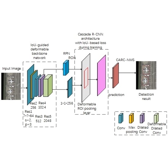
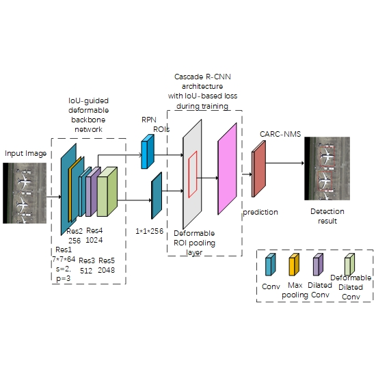
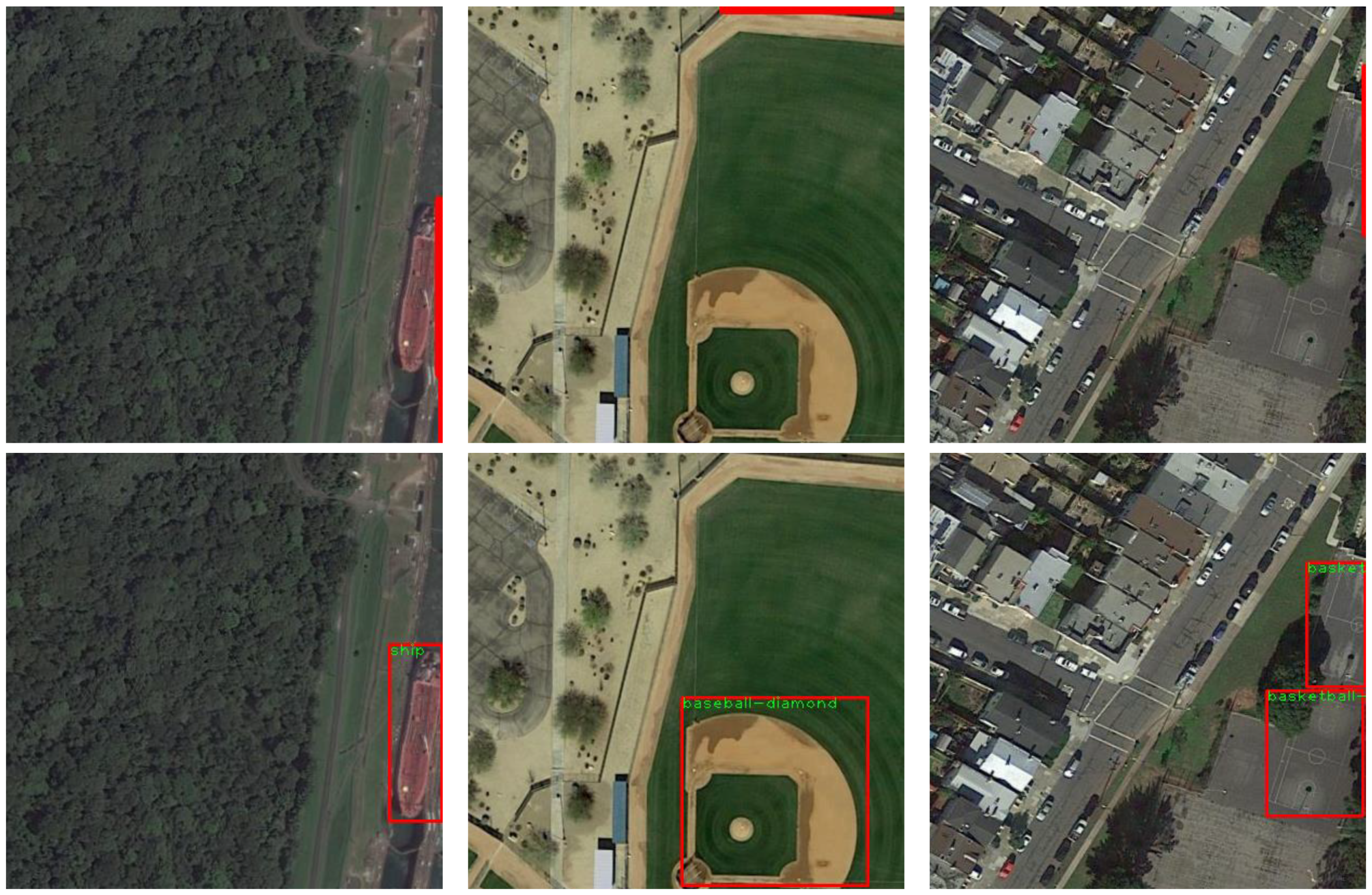
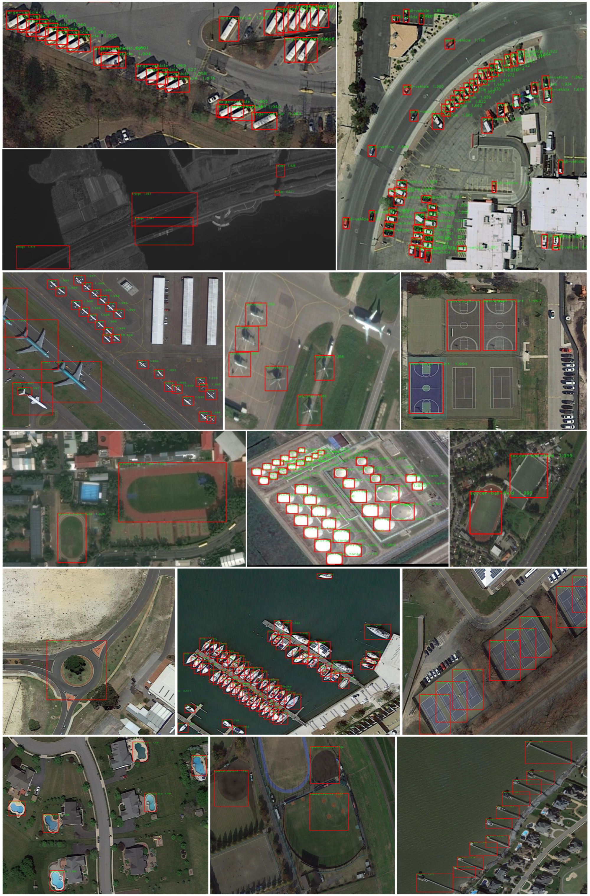
In this section, we first show different roles of IoU in the network and the effectiveness of our method with comprehensive ablation experiments. Then, we show that our approach achieves state-of-the-art results on DOTA benchmarks with the final optimal model. Our method outperforms all the published methods evaluated on the HBB prediction task benchmark. Visualization of the objects detected by IoU-Adaptive Deformable R-CNN in the DOTA dataset is shown in Figure 5. From Figure 5, IoU-Adaptive Deformable R-CNN shows satisfactory detection results in recognizing adjacent or overlapping objects such as ships, harbors, storage tanks, and ball courts. In particular, the AP values of small objects like ships, small vehicles and large vehicles increase more than other objects, which illustrate the favorable performance of our methods for small object detection.

4.1. Ablation Experiments

A couple of ablation experiments have been run to analyze the different roles of IoU in the network and the effectiveness of our method on the DOTA validation set. We use AP to evaluate the detection performance of different methods. All detectors are reimplemented with MXNet, on the same codebase released by MSRA [18] for comparison.

The impact of dilated convolutions: It can be seen from

Table 3. Quantitative comparison of the baseline and other methods on DOTA dataset We highlight in bold the best results on each category.

Method	Test_Data
Azimi et al. [23]	test	plane	BD	bridge	GTF	SV	LV	ship	TC
		89.54	73.48	51.96	70.33	73.39	67.91	78.15	90.39
		BC	ST	SBF	RA	harbor	SP	HC	mAP
		78.73	78.48	51.02	59.41	73.81	69	52.59	70.54
baseline [18]	test	plane	BD	bridge	GTF	SV	LV	ship	TC
		86.53	77.54	42.7	64.43	67.6	63.64	77.86	90.33
		BC	ST	SBF	RA	harbor	SP	HC	mAP
		77.82	75.36	52.12	56.79	68.92	62.04	54.92	67.91
baseline [18]	val_clip	plane	BD	bridge	GTF	SV	LV	ship	TC
		87.52	77.9	51.5	75.86	53.93	61.17	83.75	90.38
		BC	ST	SBF	RA	harbor	SP	HC	mAP
		57.83	51.44	65.45	57.21	77.61	49.73	62.86	66.94
baseline+dilated Conv	val_clip	plane	BD	bridge	GTF	SV	LV	ship	TC
		87.62	76.99	52.81	76.64	56.48	65.8	87.19	89.04
		BC	ST	SBF	RA	harbor	SP	HC	mAP
		58.73	62.16	66.02	58.69	76.92	51.35	70.4	69.12

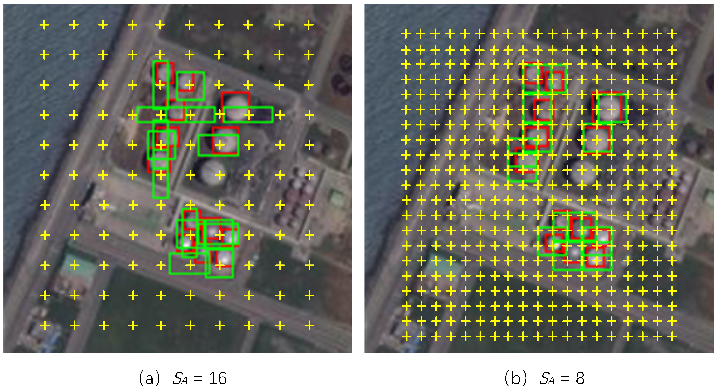
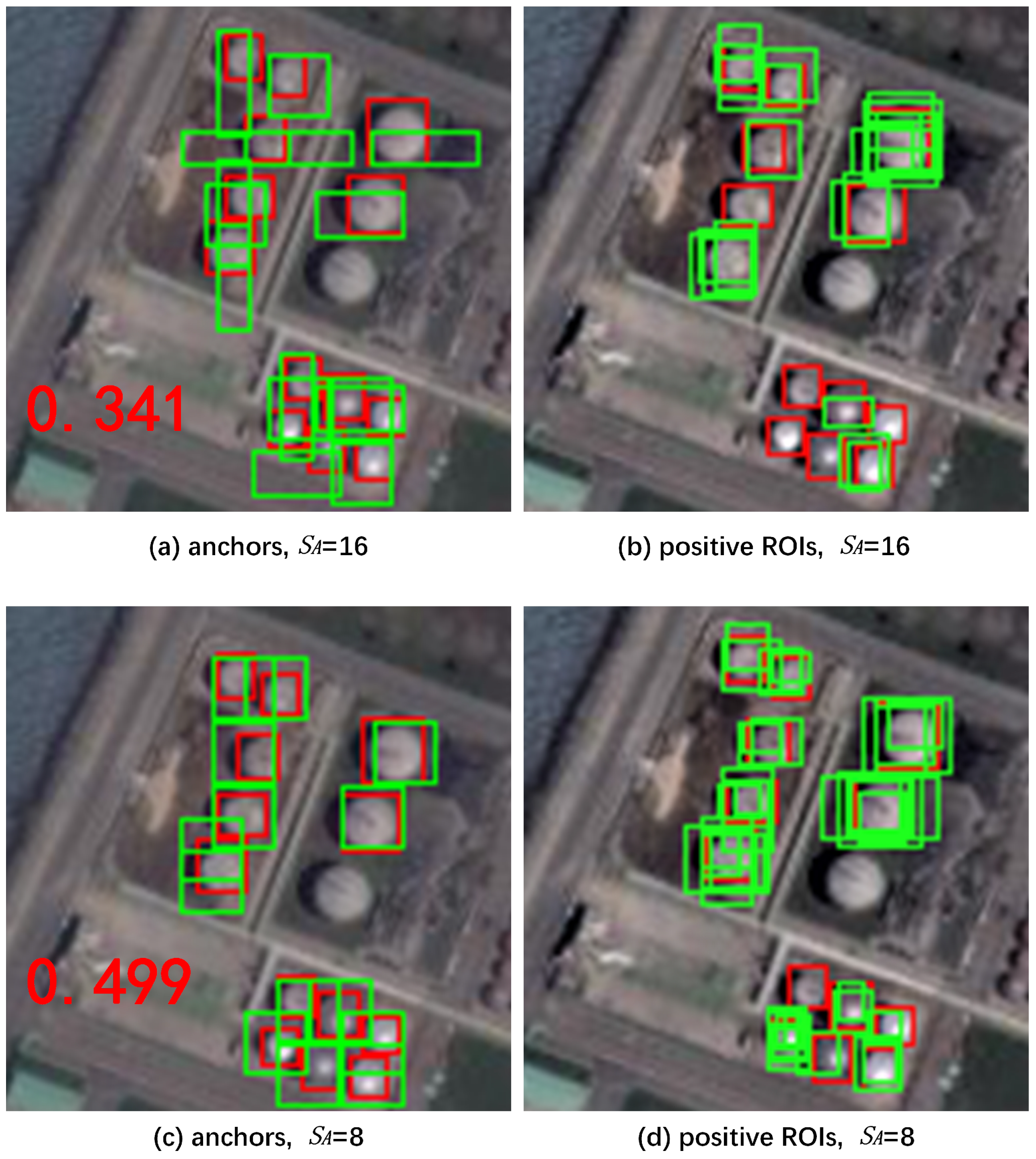
that the baseline network Deformable Faster R-CNN performs poorly on small object detection when compared with the work of Azimi et al. [23], which get the best detection results in all published methods. In order to better detect a large number of small objects in the dataset, we use the dilated convolutions in the 4th and 5th network stages of the original backbone network. On the one hand, increasing the feature map makes the object features, especially the small object features more expressive. On the other hand, compared with the previous network, increasing the anchor density enables small objects to obtain matching anchors with larger IoUs. At the same time, there are more positive ROIs corresponding to small objects participating in the training of the network. As shown in the Figure 6, we draw the GT boxes of small objects with red rectangles, and the anchors or positive ROIs corresponding to the small object with green rectangles. The number in the first column images is the average IoU of anchors corresponding to the small objects. It can be seen that when we use suitable number of dilated convolutions, the anchors and positive ROIs involved in network training are more reasonable.

By using dilated convolutions, we can obtain more reasonable anchors corresponding to small objects to participate in the training of the RPN network. In addition, as shown in Figure 6, we can get more positive ROIs corresponding to small objects to participate in the training of the detection head, and a higher recall rate can be obtained during the inference. As shown in Table 3, the detection performance of some categories, especially those with many small objects (such as ship, storage-tank) has been significantly improved. Meanwhile, the detection performance of some categories has been declined, may be due to the fact that the network generates more anchors and introduces more FPs.

The impact of reducing IoU threshold of the detectors: The quality of a detector is defined by Cai et al. [15]. Since a bounding box usually includes an object and some amount of background, it is difficult to determine a detection is positive or negative. We usually make judgment by using the IoU overlap between detection BB and the GT box. If the IoU is above a predefined threshold u, the patch is considered an example of the foreground. Thus, the class label of a hypothesis x is a function of u,

$$y=\left\{\begin{array}{cc}{g}_y,\hfill & \mathrm{if}\mathrm{IoU}(\mathrm{x},\mathrm{g})\ge u\hfill \\ 0,\hfill & \mathrm{if}\mathrm{ohterwise}\hfill \end{array}\right.$$

(15)

where $g_y$ is the class label of the GT object g and the IoU threshold defines the quality of the detector.

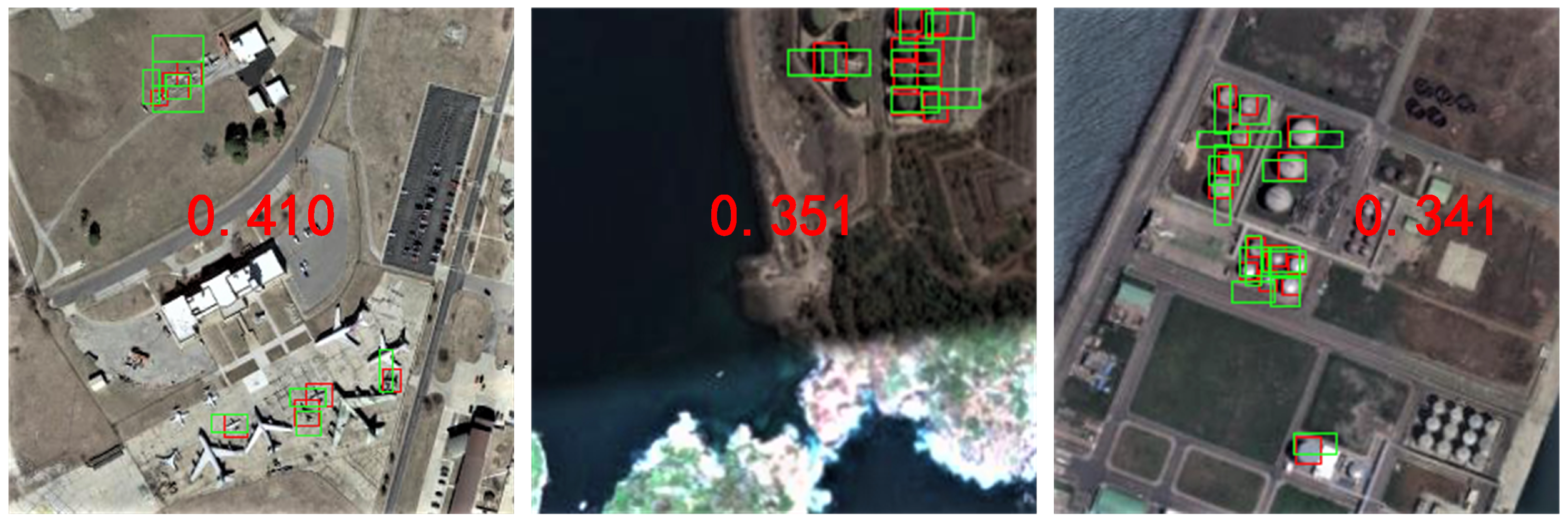
As shown in the last column of Figure 6, there are many small objects that are ignored and do not participate in the training of the network. Even if the density of the anchor is increased by using more dilated convolutions, there are still small objects lacking the corresponding positive ROIs. Therefore, we appropriately reduce the IoU threshold of the detector so that more small objects can participate in the training of the network. As shown in Figure 7, when the detector’s IoU threshold is changed from 0.5 to 0.4, more small objects participate in the training of the network. With the participation of these ROIs, which have small IoU values during training, the regression branch can make the proposal with a lower IoU regress to the position of the GT box more efficiently. The detection performance is listed in

Table 4. The effect of setting different IoU thresholds for the detector during training. We perform evaluation on the val_clip set The best results on each category is highlight in bold.

Method
baseline [18]	plane	BD	bridge	GTF	SV	LV	ship	TC
	87.52	77.9	51.5	75.86	53.93	61.17	83.75	90.38
	BC	ST	SBF	RA	harbor	SP	HC	mAP
	57.83	51.44	65.45	57.21	77.61	49.73	62.86	66.94
baseline+IoU 0.4	plane	BD	bridge	GTF	SV	LV	ship	TC
	87.7	80.69	48.81	78.01	58.09	61.75	84.89	90.18
	BC	ST	SBF	RA	harbor	SP	HC	mAP
	55.57	55.18	70.42	58.39	75.38	52.5	64.49	68.14

, for most categories, the detection performance is improved when the detector’s IoU threshold is lowered.

The impact of Cascade R-CNN architecture: Although the use of dilated convolutions and lowering the IoU threshold of the detector can effectively improve the ability of the network to handle small object detection problems, it may reduce the detection performance of other objects due to the reasons indicated in Section 2.1.

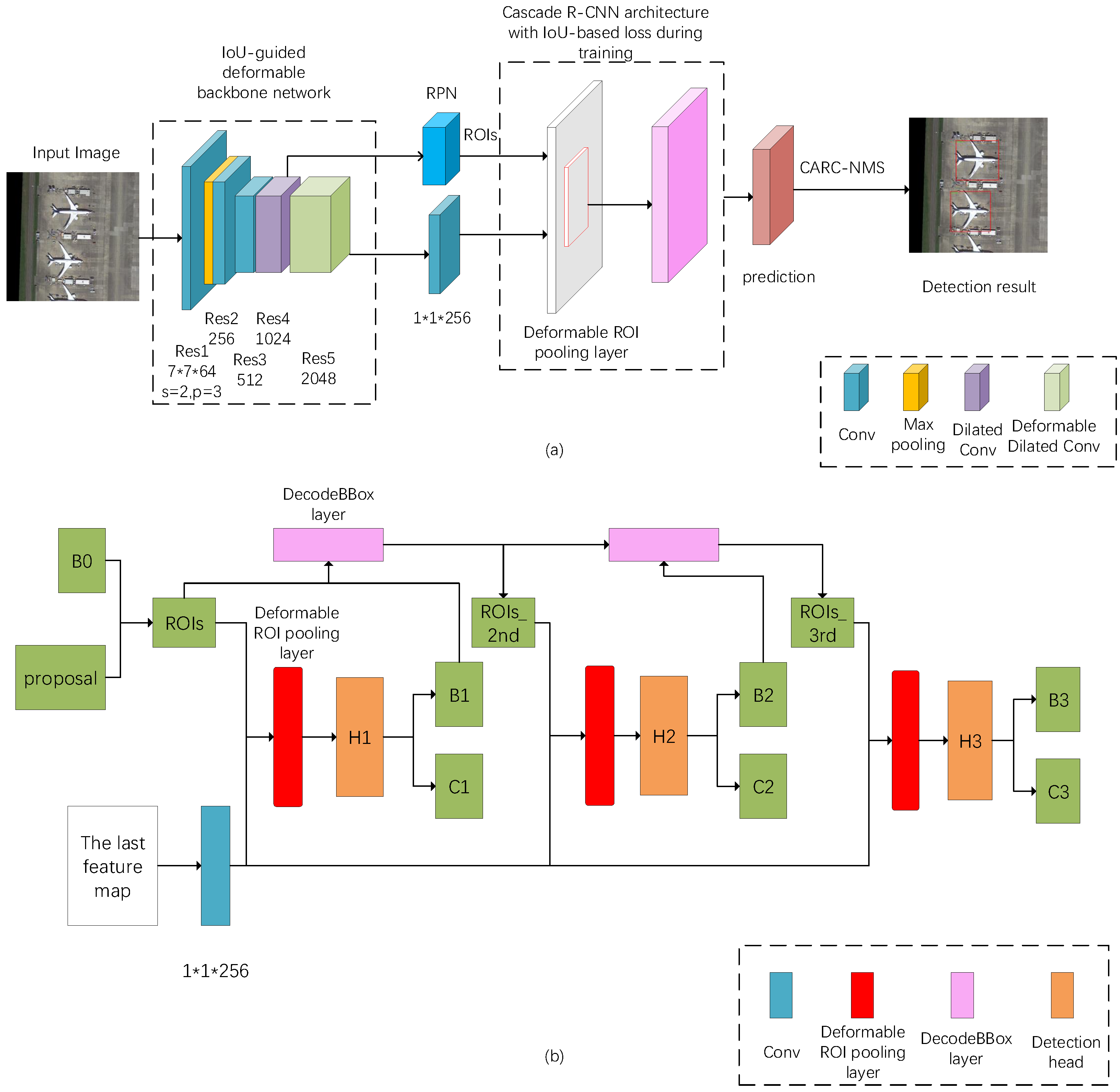
As compensation, we use the Cascaded R-CNN architecture to improve the overall detection performance. Additional cascading of two detection heads of the same structure with increasing IoU thresholds based on the original detection head structure, we get more accurate detection results, and the detection results can get closer to the corresponding GT boxes through multiple regression. In addition, more True Positive results can be obtained when used the Cascaded R-CNN architecture. It is helpful to improve the overall detection performance as shown in

Table 5. The impact of Cascade R-CNN architecture, we evaluate on val set.

Method		Plane	BD	Bridge	GTF	SV	LV	Ship	TC
baseline+0.4	AP	86.67	69.54	40.55	60.92	53.22	63.78	84.01	90.13
	TP	2365	181	316	116	4587	3626	8047	710
	FP	12,090	2397	21,798	3792	123,132	76,126	42,921	5041
baseline+0.4+dilated	AP	86.43	67.62	44.02	64.55	49.48	61.22	85.42	88.91
	TP	2366	185	310	113	4733	3623	8205	698
	FP	6197	2020	7188	3513	87,227	50,905	26,622	4078
baseline+0.4+dilated+Cascade	AP	86.78	66.99	41.87	57.76	64.13	68.21	87.41	89.89
	TP	2351	189	306	115	4873	3673	8306	711
	FP	6993	3598	8809	5135	89,094	53,290	30,331	4737
Method		BC	ST	SBF	RA	Harbor	SP	HC	mAP
baseline+0.4	AP	65.85	82.14	66.56	62.64	70.76	50.34	55.29	66.83
	TP	102	1724	78	140	1812	294	61	−
	FP	3593	31,486	2526	4755	16,118	10,746	3920	−
baseline+0.4+dilated	AP	63.13	78.53	70.14	64.83	69.35	46.29	58.28	66.55
	TP	97	1755	80	138	1815	292	61	−
	FP	2131	19,672	1820	2745	12,758	6197	2556	−
baseline+0.4+dilated+Cascade	AP	63.86	81.72	70.01	59.37	70.77	53.4	55.36	67.83
	TP	101	1765	83	139	1827	300	62	−
	FP	3392	16,102	2666	3820	14,643	6456	3079	−

.

The impact of the IoU-based Weighted Loss: To the best of our knowledge, we are the first to propose that the loss function can be weighted by the IoU value of the ROI during training to improve the detection performance. In order to analyze the different effects on classification branch and regression branch when we introduce the influence of the IoU weighting function, we designed three different loss functions based on the basic framework to introduce the impact of the IoU value on the network learning. Results in

Table 6. The impact of the IoU-based Weighted Loss.we evaluate on val set.

Method	Plane	BD	Bridge	GTF	SV	LV	Ship	TC
baseline [18]	86.67	69.54	40.55	60.92	53.22	63.78	84.01	90.13
baseline+iou based cls_loss	88.26	70.1	48.28	68.12	61.88	69.29	82.77	90.5
baseline+iou based bbox_loss	88.69	70.86	48.37	65.02	62.98	70.54	83.13	90.52
baseline+iou based loss	89.04	65.67	48.42	67.18	65.14	70.86	83.65	90.48
Method	BC	ST	SBF	RA	Harbor	SP	HC	mAP
baseline [18]	65.85	82.14	66.56	62.64	70.76	50.34	55.29	66.83
baseline+iou based cls_loss	66.41	85.69	68.97	66.91	74.96	53.51	60.44	70.41
baseline+iou based bbox_loss	67.57	85.14	72.04	67.33	75.22	56.6	59.06	70.87
baseline+iou based loss	66.11	86.52	67.72	67.17	75.31	53	56.23	70.17

show that all three weighted loss functions improve the detection accuracy. There is no significant difference in the final detection performance when we used three different loss functions for training. In the following experiments, we use the IoU weighted loss function that affects both the classification branch and the regression branch by default.

To analyze the impact of using different weighting method on detection performance, we also use other weight calculation formulas. For example, we change the weight of the classification loss as $0.5+iou$ when a positive ROI has an IoU larger than 0.5, which remove the problem of weight jump changes existing in Equation (7), but there is no significant difference in the final detection performance (the mAP is 70.41 when use Equation (7) while the mAP is 70.47 when we use the new weight calculation formula). Furthermore, we change the weight of the regression loss as $1.5-iou$ or $3-iou$ during training when a positive ROI has an IoU larger than the IoU threshold of the detector. As the weight value increases, the detection performance has a small increase as shown in

Table 7. The impact of using different weight calculation formulas. We have designed three different regression loss weight calculation formula, and we evaluate on val set, The best results on each category is highlight in bold.

Weight Calculation Formula	Plane	BD	Bridge	GTF	SV	LV	Ship	TC
$1.5-iou$	89.07	70.46	47.59	63.67	62.85	74.43	84.51	90.34
$2-iou$ (Equation (8))	88.69	70.86	48.37	65.02	62.98	70.54	83.13	90.52
$3-iou$	88.37	71.13	48.43	65.13	65.13	74.85	85.77	90.52
Weight Calculation Formula	BC	ST	SBF	RA	Harbor	SP	HC	mAP
$1.5-iou$	67.21	84.37	71.47	64.87	74.46	55.83	55.71	70.45
$2-iou$ (Equation (8))	67.57	85.14	72.04	67.33	75.22	56.6	59.06	70.87
$3-iou$	70.08	86.37	65.11	64.42	75.09	56.13	57.84	70.96

. A more reasonable weight calculation method will be studied in our future work.

The impact of the Class Aspect Ratio Constrained NMS (CARC-NMS): As shown in

Table 8. The mean, standard deviation, and corresponding constraint factors of the distribution of different classes of samples L_AR.

	Plane	BD	Bridge	GTF	SV	LV	Ship	TC
mean	0	0	0.015	−0.06	−0.01	0.022	0.022	−0.17
std	0.11	0.081	0.252	0.189	0.197	0.305	0.275	0.14
m	4.887	4.487	4.35	3.753	3.107	3.194	3.364	4.86
	BC	ST	SBF	RA	Harbor	SP	HC	−
mean	−0.103	0	−0.04	0	−0.06	0.023	−0.345	−
std	0.167	0.063	0.167	0.072	0.32	0.168	0.237	−
m	3.789	4.86	3.355	4.53	3.86	3.33	4.746	−

, we list the mean, standard deviation, and corresponding constraint factors of the distribution of different classes of samples $L\_ARs$ which are calculated according to the annotations of the training set. When evaluated on the test set, our final detection framework used CARC-NMS instead of NMS can lead to an additional increase of 0.8% for the mean average precision metric (from 71.93% to 72.72%), and an average 0.8% performance gain can be get when we evaluated on the validation set.

4.2. Comparison With the State-of-the-Art

Table 9. Quantitative comparison of the baseline and our method on the HBB task in test set of DOTA dataset FR-H stands for Faster R-CNN[6] trained on HBB. The best results on each category is highlight in bold.

	YOLOv2 [25]	R-FCN [11]	SSD [26]	FR-H [9]	Deformable FR-H [18]	Azimi et al. [23]	Ours
plane	76.90	81.01	57.85	80.32	86.53	89.97	88.62
BD	33.87	58.96	32.79	77.55	77.54	77.71	80.22
bridge	22.73	31.64	16.14	32.86	42.7	53.38	53.18
GTF	34.88	58.97	18.67	68.13	64.43	73.26	66.97
SV	38.73	49.77	0.05	53.66	67.6	73.46	76.3
LV	32.02	45.04	36.93	52.49	63.64	65.02	72.59
ship	52.37	49.29	24.74	50.04	77.86	78.22	84.07
TC	61.65	68.99	81.16	90.41	90.33	90.79	90.66
BC	48.54	52.07	25.1	75.05	77.82	79.05	80.95
ST	33.91	67.42	47.47	59.59	75.36	84.81	76.24
SBF	29.27	41.83	11.22	57.00	52.12	57.20	57.12
RA	36.83	51.44	31.53	49.81	56.79	62.11	66.65
harbor	36.44	45.15	14.12	61.69	68.92	73.45	74.08
SP	38.26	53.3	9.09	56.46	62.04	70.22	66.36
HC	11.61	33.89	0.0	41.85	54.92	58.08	56.85
mAP	39.20	52.58	29.86	60.64	67.91	72.45	72.72

shows the performance of our algorithm on the HBB prediction tasks of the DOTA dataset. In order to get a better results, we changed the NMS threshold of the LV and ship categories from 0.3 to 0.4 when testing on the test subset. In the case of not using multi-scale training and multi-scale testing, feature pyramid structure, rotational region-proposal network (R-RPN) and Online Hard Positive Mining (OHEM), which can further improve the performance of the network, we achieve the state-of-the-art detection performance on the DOTA dataset and achieve significant improvements in comparison with the baseline network. Compared to the baseline network, there is a 4.8% increase for the overall detection performance, and we have achieved better results in all categories, and compared with the method proposed by Azimi et al., which gets the best detection result in all published algorithms, we achieve the same detection result without introducing image pyramid and feature pyramid, and these two strategies can also be applied to our method to further improve the detection performance. Using image pyramid is helpful to solve the detection problem when the target is larger than the cropped image size.

5. Discussion

The experimental results have shown that our method can achieve desirable results without bells and whistles. Compared to other published methods, our detection framework achieves the best mAP for HBB detection tasks on DOTA dataset With the IoU-guided detection framework, the problem of loss of small object information during training is effectively solved, and we achieve a better overall detection performance with the IoU-based weighted loss we proposed. Finally, our detection framework outperforms the baseline network by 4.81 points mAP. When compared to the work of Azimi et al. [23], which gets the best detection results in all published methods, we get a better detection performance on the classes with more small objects, such as small vehicle, large vehicle, ship and so on, but the detection performance of ground-track-field, storage tank and swimming pool is lower than that shown by Azimi et al. We think the new joint image cascade and feature pyramid network proposed by them can provide great help in detecting these classes of samples, which we can use to further improve our network.

In addition, the network can get further improvements. As the weight calculation formula based on IoU is designed in a very simple way. By using a more reasonable weighting method, the detection performance of the network can be further improved. Furthermore, for a 800 × 800 image, the baseline network takes 0.22 s for detection. As we use more dilated convolutions and the Cascade R-CNN architecture, the detection speed of the network is significantly lower than baseline network, which takes 0.95 s for detection. We will conduct further research on how to design more efficient weighting methods and how to improve the detection efficiency of the network in our future work.

6. Conclusions

In this paper, we analyzed the role that IoU can play in a two-stage detection networks, and based on this, we proposed a new algorithm for multi-class object detection in unconstrained RS imagery and evaluated it on DOTA datasets. Our algorithm uses suitable dilated convolutions in the backbone network and a smaller IoU threshold for detectors, which are significant for detecting small objects, and we solved the loss of small objects information problem during training to some extent. Furthermore, we enhance our model by applying Cascade R-CNN architecture and propose the IoU-based Weighted loss during training to improve the overall detection performance. Finally, we use CARC-NMS for post processing. Our method outperforms the baseline network by a large margin and achieve the state-of-the-art detection performance showed in other published algorithms [3,23] on the DOTA dataset. Our approach is robust to differences in spatial resolution of the image data acquired by various platforms (airborne and space-borne). For future work, we plan to further apply our proposed method to the detection tasks with oriented bounding boxes and use Scale Normalization for Image Pyramids (SNIP) methods to further improve network performance with multi-scale training and multi-scale testing at a small cost.

References

1. Yang, X.; Sun, H.; Fu, K.; Yang, J.; Sun, X.; Yan, M.; Guo, Z. Automatic Ship Detection in Remote Sensing Images from Google Earth of Complex Scenes Based on Multiscale Rotation Dense Feature Pyramid Networks. Remote Sens. 2018, 10, 132. [Google Scholar] [CrossRef]
2. Yang, X.; Sun, H.; Sun, X.; Yan, M.; Guo, Z.; Fu, K. Position Detection and Direction Prediction for Arbitrary-Oriented Ships via Multiscale Rotation Region Convolutional Neural Network. 2018. Available online: https://arxiv.org/ftp/arxiv/papers/1806/1806.04828.pdf (accessed on 27 January 2019).
3. Xia, G.; Bai, X.; Ding, J.; Zhu, Z.; Belongie, S.J.; Luo, J.; Datcu, M.; Pelillo, M.; Zhang, L. DOTA: A Large-Scale Dataset for Object Detection in Aerial Images. In Proceedings of the Computer Vision and Pattern Recognition, Salt Lake City, UT, USA, 18–22 June 2018; pp. 3974–3983. [Google Scholar]
4. Cheng, G.; Zhou, P.; Han, J. Learning Rotation-Invariant Convolutional Neural Networks for Object Detection in VHR Optical Remote Sensing Images. IEEE Trans. Geosci. Remote Sens. 2016, 54, 7405–7415. [Google Scholar] [CrossRef]
5. Han, X.; Zhong, Y.; Zhang, L. An Efficient and Robust Integrated Geospatial Object Detection Framework for High Spatial Resolution Remote Sensing Imagery. Remote Sens. 2017, 9, 666. [Google Scholar] [CrossRef]
6. Xu, Z.; Xu, X.; Wang, L.; Yang, R.; Pu, F. Deformable ConvNet with Aspect Ratio Constrained NMS for Object Detection in Remote Sensing Imagery. Remote Sens. 2017, 9, 1312. [Google Scholar] [CrossRef]
7. Zhong, Y.; Han, X.; Zhang, L. Multi-class geospatial object detection based on a position-sensitive balancing framework for high spatial resolution Remote Sensing imagery. Isprs J. Photogramm. Remote Sens. 2018, 138, 281–294. [Google Scholar] [CrossRef]
8. Guo, W.; Yang, W.; Zhang, H.; Hua, G. Geospatial Object Detection in High Resolution Satellite Images Based on Multi-Scale Convolutional Neural Network. Remote Sens. 2018, 10, 131. [Google Scholar] [CrossRef]
9. Ren, S.; He, K.; Girshick, R.B.; Sun, J. Faster R-CNN: Towards real-time object detection with region proposal networks. arXiv, 2015; arXiv:1506.01497. [Google Scholar] [CrossRef] [PubMed]
10. Chen, L.; Papandreou, G.; Kokkinos, I.; Murphy, K.P.; Yuille, A.L. DeepLab: Semantic Image Segmentation with Deep Convolutional Nets, Atrous Convolution, and Fully Connected CRFs. IEEE Trans. Pattern Anal. Mach. Intell. 2018, 40, 834–848. [Google Scholar] [CrossRef] [PubMed] [Green Version]
11. Dai, J.; Li, Y.; He, K.; Sun, J. R-FCN: Object Detection via Region-based Fully Convolutional Networks. Neural Inf. Process. Syst. 2016, 379–387. [Google Scholar]
12. Ren, Y.; Zhu, C.; Xiao, S. Deformable Faster R-CNN with Aggregating Multi-Layer Features for Partially Occluded Object Detection in Optical Remote Sensing Images. Remote Sens. 2018, 10, 1470. [Google Scholar] [CrossRef]
13. Zagoruyko, S.; Lerer, A.; Lin, T.; Pinheiro, P.H.O.; Gross, S.; Chintala, S.; Dollar, P. A MultiPath Network for Object Detection. In Proceedings of the British Machine Vision Conference, York, UK, 19–22 September 2016. [Google Scholar]
14. Xu, Y.; Zhu, M.; Li, S.; Feng, H.; Ma, S.; Che, J. End-to-End Airport Detection in Remote Sensing Images Combining Cascade Region Proposal Networks and Multi-Threshold Detection Networks. Remote Sens. 2018, 10, 1516. [Google Scholar] [CrossRef]
15. Cai, Z.; Vasconcelos, N. Cascade R-CNN: Delving Into High Quality Object Detection. In Proceedings of the Computer Vision and Pattern Recognition, Salt Lake City, UT, USA, 18–22 June 2018; pp. 6154–6162. [Google Scholar]
16. Singh, B.; Davis, L.S. An Analysis of Scale Invariance in Object Detection—SNIP. In Proceedings of the Computer Vision and Pattern Recognition, Salt Lake City, UT, USA, 18–22 June 2018. [Google Scholar]
17. Zhu, C.; Tao, R.; Luu, K.; Savvides, M. Seeing Small Faces From Robust Anchor’s Perspective. In Proceedings of the Computer Vision and Pattern Recognition, Salt Lake City, UT, USA, 18–22 June 2018. [Google Scholar]
18. Dai, J.; Qi, H.; Xiong, Y.; Li, Y.; Zhang, G.; Hu, H.; Wei, Y. Deformable Convolutional Networks. In Proceedings of the International Conference on Computer Vision, Venice, Italy, 22–29 October 2017; pp. 764–773. [Google Scholar]
19. Zhu, H.; Chen, X.; Dai, W.; Fu, K.; Ye, Q.; Jiao, J. Orientation robust object detection in aerial images using deep convolutional neural network. In Proceedings of the 2015 IEEE International Conference on Image Processing (ICIP), Quebec City, QC, Canada, 27–30 September 2015; pp. 3735–3739. [Google Scholar]
20. Liu, K.; Mattyus, G. Fast Multiclass Vehicle Detection on Aerial Images. IEEE Geosci. Remote Sens. Lett. 2015, 12, 1938–1942. [Google Scholar]
21. Liu, Z.; Wang, H.; Weng, L.; Yang, Y. Ship Rotated Bounding Box Space for Ship Extraction From High-Resolution Optical Satellite Images with Complex Backgrounds. IEEE Geosci. Remote Sens. Lett. 2016, 13, 1074–1078. [Google Scholar] [CrossRef]
22. Razakarivony, S.; Jurie, F. Vehicle detection in aerial imagery: A small target detection benchmark. J. Vis. Commun. Image Represent. 2015, 34, 187–203. [Google Scholar] [CrossRef]
23. Azimi, S.M.; Vig, E.; Bahmanyar, R.; Korner, M.; Reinartz, P. Towards Multi-class Object Detection in Unconstrained Remote Sensing Imagery. arXiv, 2018; arXiv:1807.02700. [Google Scholar]
24. Deng, J.; Dong, W.; Socher, R.; Li, L.; Li, K.; Feifei, L. ImageNet: A large-scale hierarchical image database. In Proceedings of the Computer Vision and Pattern Recognition, Miami, FL, USA, 25 June 2009; pp. 248–255. [Google Scholar]
25. Redmon, J.; Farhadi, A. YOLO9000: Better, Faster, Stronger. arXiv, 2017; arXiv:1612.08242. [Google Scholar]
26. Liu, W.; Anguelov, D.; Erhan, D.; Szegedy, C.; Reed, S.; Fu, C.Y.; Berg, A.C. SSD: Single Shot MultiBox Detector. In Proceedings of the European Conference on Computer Vision, Amsterdam, The Netherlands, 8–16 October 2016; pp. 21–37. [Google Scholar]
Figure 1. Anchor sampling in different S A . S A mean the stride of the anchors in different detection framework. The green bounding box represents the anchor, the red represents ground-truth.
Remotesensing 11 00286 g001
Figure 2. Small objects in the dataset and their corresponding positive anchors under the Faster R-CNN framework. The GT box is represented by a red rectangle, and the positive anchors corresponding to the GT box are represented by green rectangles. Numbers in the images are the average IoUs of the positive anchors corresponding to the small objects.
Remotesensing 11 00286 g002
Figure 3. (a) An overview of the IoU-Adaptive Deformable R-CNN (b) The deformable Cascade R-CNN architecture. We set the IoU threshold value of detection head H1, H2, H3 to 0.4, 0.5, 0.6 respectively in our framework. “H” network head, “B” bounding box offset, and “C” classification. “B0” is offset of proposals in image (b).
Remotesensing 11 00286 g003
Figure 4. Illustration of lines like false region proposals (LFRP, the first row) generated by classic deformable ConvNets.
Remotesensing 11 00286 g004
Figure 5. Outputs of HBB prediction on test images of DOTA dataset.
Remotesensing 11 00286 g005
Figure 6. Anchors and positive ROIs which participate in network training. S A mean the stride of the anchors in different detection framework. When we use dilated convolution in Res5 stage, S A = 16 as shown in the first row images. When we use dilated convolution in Res4 and Res5 stage, S A = 8 as shown in the second row images. The green bounding box represents the anchor or positive ROI, the red represents ground truth. Numbers in the first column images are the average IoU value of the positive anchors corresponding to the small objects exist in this image.
Remotesensing 11 00286 g006
Figure 7. The positive ROIs and the prediction results when we used different IoU threshold to train the detection framework. (a,b) shows the positive ROIs corresponding to small objects participating in network training when the IoU threshold is set to 0.5 and 0.4, respectively, and (c,d) shows the prediction results of the baseline network and the network which used more dilated convolutions and a lower IoU threshold. The GT box is represented by a red rectangle, and the positive ROIs corresponding to the GT box or detection results are represented by green rectangles. It can be seen that when the IoU threshold is set to 0.4, there are more small objects involved in network training and the test result gets a higher recall rate.
Remotesensing 11 00286 g007