Abstract
Lake Malawi is an important water resource in Africa. However, there is no routine monitoring of water quality in the lake due to financial and institutional constraints in the surrounding countries. A combination of satellite data and a semi-analytical algorithm can provide an alternative for routine monitoring of water quality, especially in developing countries. In this study, we first compared the performance of two semi-analytical algorithms, Doron11 and Lee15, which can estimate Secchi disk depth (SD) from satellite data in Lake Malawi. Our results showed that even though the SD estimations from the two algorithms were very highly correlated, the Lee15 outperformed the Doron11 in Lake Malawi with high estimation accuracy (RMSE = 1.17 m, MAPE = 18.7%, R = 0.66, p < 0.05). We then evaluated water transparency in Lake Malawi using the SD values estimated from nine years of Medium Resolution Imaging Spectrometer (MERIS) data (2003–2011) with the Lee15 algorithm. Results showed that Lake Malawi maintained four water transparency levels throughout the study period (i.e., level 1: SD > 12 m; level 2: SD between 6–12 m; level 3: SD between 3–6 m; level 4: SD between 1.5–3 m). The level 1 and 2 water areas tended to shift or trade places depending on year or season. In contrast, level 3 and 4 water areas were relatively stable and constantly distributed along the southwestern and southern lakeshores. In general, Lake Malawi is dominated by waters with SD values larger than 6 m (>95%). This study represents the first overall and comprehensive analysis of water transparency status and spatiotemporal variation in Lake Malawi.
1. Introduction
Lake Malawi, with an area of 29,252 km2, is the third largest lake in Africa and the ninth largest in the world, if the Aral Sea is excluded [1]. The lake serves as an important water resource, providing economic, recreational, and domestic uses for riparian countries [2]. In addition, the lake has the largest number of indigenous fish species in the world, and thus conservation of the biodiversity in the lake is important [3]. However, given the steady population growth of the riparian countries, and land use conversion from forests to agriculture in the watershed of the lake, water quality in Lake Malawi has been deteriorating [4,5]. Therefore, routine monitoring of water quality is essential.
Generally, two main techniques are used for monitoring water quality: (1) field survey by a boat; and (2) using remote sensing data. However, financial and institutional constraints in Africa make for poor availability of in situ water quality data in most African lakes [6]. In addition, in situ monitoring of a large lake such as Lake Malawi has spatial constraints, which makes it difficult to represent the characteristics of water quality across the entire lake. Therefore, the remote sensing technique should be considered as an effective method for providing water quality information on African lakes, especially for monitoring a big lake such as Lake Malawi [6,7].
There are two requirements for monitoring water quality by the remote sensing technique. First, a satellite sensor with ocean bands is desired. These include, for example, the Sea-viewing Wide Field-of-view Sensor (SeaWiFS) and Moderate Resolution Imaging Spectroradiometer (MODIS) from the National Aeronautics and Space Administration (NASA), and the Medium Resolution Imaging Spectrometer (MERIS) from the European Space Agency (ESA) [8]. Compared to sensors for land applications, the ocean color sensors can provide remote sensing reflectance (Rrs) data with better temporal and spectral resolution, as well as higher radiative sensitivity, all of which are necessary for monitoring water quality [9].
Second, an algorithm is needed for estimating water quality parameters from the Rrs. The algorithm can be either empirical or semi-analytical. Although empirical algorithms are easy to implement, in situ data for recalibration is always necessary, which limits their applicability to other lakes, especially those without available in situ data. In contrast, semi-analytical algorithms are based on a radiative transfer theory (or bio-optical model) with several secondary important empirical relationships under some assumptions, and thus do not often require recalibration [10,11]. In cases where there is a lack of in situ data such as in Lake Malawi, the use of a semi-analytical algorithm is the most practical and viable method for estimating water quality parameters.
The main water quality parameters that can be estimated from remote sensing data using the semi-analytical algorithms are Chlorophyll-a (Chl-a, [12,13,14]), total suspended matter (TSM; [15]), colored dissolved organic matter (CDOM, [14]), and Secchi disk depth (SD, [11,16]). As the SD estimation is based on an underwater visibility theory, and the SD value itself is an apparent optical property (AOP) of a water body just like Rrs, the relationship between SD and Rrs values can be considered more robust than those between other water quality parameters and Rrs values. In addition, the SD value is easy to measure and can be understood by the general public. Thus, it has been widely used as an indicator for evaluating water quality (transparency or clarity) since the 1860s [17] as well as one of the important parameters for calculating trophic state index (TSI, [18]).
There are two main semi-analytical algorithms for estimating SD values from remote sensing data. The first, developed by Doron et al. in 2011 [16], is based on a classic underwater visibility theory that has been used for over 60 years ([19]; hereafter, ‘Doron11’). The second semi-analytical algorithm was developed by Lee et al. in 2015, based on a new underwater visibility theory proposed by the same authors in the same study ([11]; hereafter, ‘Lee15’). Although Lee et al. [11] pointed out some shortcomings in the classic theory, and later [20] directly compared the performance of Doron11 and Lee15 using a simulated dataset, the two algorithms have not been applied in practice to the same water body and compared to common in situ measured SD values. Therefore, we considered that there was not yet enough evidence to show which algorithm should be selected and used in Lake Malawi.
In consideration of the above, and the fact that few studies have comprehensively evaluated water quality in Lake Malawi [5,21], the research objectives of the present study are: (1) to comprehensively compare the performance of the two semi-analytical algorithms (Doron11 and Lee15) in Lake Malawi; and (2) to obtain an overall evaluation of water transparency in Lake Malawi from MERIS data.
2. Materials and Methods
2.1. Study Area
Lake Malawi (09°30′–14°40′S, 33°50′–33°36′E) is the southernmost lake in the Great Rift Valley, surrounded by Malawi, Mozambique, and Tanzania (Figure 1). While the lake is also known as Niassa in Mozambique and Nyasa in Tanzania, internationally and scientifically it is known as Lake Malawi. It is about 560 km long, and has a maximum width of about 75–87 km, an average depth of 292 m, and a maximum depth of 706 m. There are three seasons in the area surrounding the lake, determined by rainfall and temperature. They are the cool dry season (May–August), hot dry season (September–October), and warm wet season (November–April), with 95% of precipitation falling during this latter period (Figure 2, [22]). The majority of the lake’s catchment is in Malawi, where the population has doubled in the past 25 years, with a 2.8% yearly increase over the last 10 years for a current total population of about 19 million. Most of the population relies directly on subsistence agriculture and fish for food, and the high population density is resulting in the expansion of subsistence agriculture to marginal land, including wetlands and steep hill slopes [23]. About 7% of the catchment area is within Mozambique, while approximately 25% lies within Tanzania; the remainder is in Malawi. Most of the rain falls along the lake’s shoreline, which is dominated by flat land contrary to other regions of the basin. All three adjacent countries are developing, and subsistence agriculture is still vital to the majority of the population.
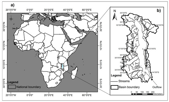
Figure 1.
Location of Lake Malawi and its watershed; the lake includs 13 main inflows and only 1 outflow (modified from [4]) (a) Geographical location of Lake Malawi (b) Lake Malawi basin including its adjacent countries.
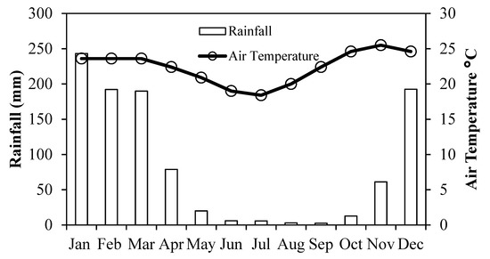
Figure 2.
Monthly mean temperature and rainfall in Malawi (1991–2015). There are three seasons: the cool dry season (May–August), hot dry season (September–October), and warm wet season (November–April). Data source: [24].
2.2. Data Collection
A total of 1658 MERIS L1b, Full Resolution (300 m) images covering the study area during 2003–2012 were downloaded from the European Space Agency (ESA, [25]). These data were subset to the lake’s basin area to reduce their size. After removing cloud-contaminated images, only 822 images from 20 Jan., 2003 to 30 Dec., 2011, were used, of which 338 images covered just half or more of the lake area. Table 1 summarizes the MERIS dataset used in this study.

Table 1.
Temporal availability of Medium Resolution Imaging Spectrometer (MERIS) images used in this study.
The Case-2 regional processor (C2R) embedded in BEAM 5.0 was used to carry out the atmospheric correction. The C2R was chosen because it has been tested over a wide range of atmospheric parameters (aerosol optical properties), and it provides atmospheric correction, smile correction, land masking through its land detection, cloud and ice invalid pixels, and other flags for filtering the data [26,27,28]. To further avoid a possible influence from the bottom reflectance caused by the pixels along the shoreline, a 600 m buffer was generated to mask these pixels. After SD estimations, the daily SD values were aggregated into monthly (averaged 9-year SD values in each month) and yearly (averaged 12-month SD values in each year) datasets.
The in situ measured SD values used in this study were collected in 2007. Figure 3 shows the sampling locations. The SD values were measured along a 10-km south–north transect. The transect included one station (KGC) at the center of the cage farm (fish cages deployed in 2004 for fish aquaculture), 4 stations at the south (CS1–CS4), and 4 stations at the north of the cage farm (CN1–CN4). The distance between two stations was controlled to be at least 1 km away [29]. The name of stations and the number of in situ SD measurements for each station including the minimum and maximum SD values are summarized in Table 2.
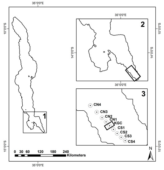
Figure 3.
Sampling locations in the southeast arm of Lake Malawi. KGC represents the center of the cage farm, CN1–CN4 represents four sampling stations in the north of KGC, and CS1–CS4 represents four sampling stations in the south of KGC (modified from [29]).
Table 2.
Stations and number of in situ Secchi disk (SD) measurements used for validation, including minimum and maximum values. KGC represents the center of the cage farm, CN1–CN4 represents four sampling stations in the north of KGC, and CS1–CS4 represents four sampling stations in the south of KGC [29].
2.3. The Two Semi-Analytical Algorithms Used in This Study
2.3.1. Doron11 Algorithm
The basic equation of the Doron11 is as follows [30,31]:
where
is the photopic vertical diffuse attenuation coefficient (m−1), is the photopic beam attenuation coefficient (m−1), is the minimum apparent contrast perceivable by the human eye (=0.0066), and is the inherent contrast between the disk and background water, which can be expressed as [30]:
where RSD is the reflectance of the Secchi disk (= 0.82 based on [30]), and is the irradiance reflectance of the environment around the Secchi disk at 490 nm.
+ can be estimated from (490) + (490) together, based on the following equation [16,20,32]:
where X represents (490) + (490), which are the vertical diffuse attenuation coefficient and beam attenuation coefficient at a wavelength of 490 nm, respectively. The (490) can be further obtained from the sum of the total absorption coefficient and total scattering coefficient at 490 nm (i.e., a(490) and b(490)); a(490) and the total backscattering coefficient at 490 nm (i.e., bb(490)) can be calculated using Equations (11) and (12) in [16] (also see Equations (A1) and (A2) in Appendix A). The b(490) can be calculated from the sum of the particle scattering coefficient (Equation (9) in [32], also see Equation (A3) in Appendix A) and the scattering coefficient of pure water at a wavelength of 490 nm.
(490) can be estimated from a(490) and bb(490) using the following equation [33]:
where
represents the solar zenith angle in degree and bbw is the backscattering coefficient of pure water [34].
2.3.2. Lee15 Algorithm
The basic equation of the Lee15 algorithm is as follows [11]:
where
is the above-water remote sensing reflectance (Rrs) corresponding to the wavelength with the minimum , and is the contrast threshold of the human eye in radiance reflectance (=0.013 sr−1). Min( (443, 490, 510, 560, 620, 665) is the at MERIS visible bands with a minimum value. The at a given band can be estimated from a and bb at the same band using Equation (4) above. In the Lee15 algorithm, the total absorption coefficient (a) and total backscattering coefficient (bb) were estimated from Rrs using the sixth version of the quasi-analytical algorithm [35].
2.4. Definition of Transparency Levels
The Organization for Economic Cooperation and Development (OECD) [36] classification system was used to define water transparency levels in Lake Malawi. In all, there are five transparency levels according to thresholds of SD values [36], which were also linked to trophic states of a water body (Table 3).
Table 3.
Transparency level definition according to thresholds of SD values [36].
2.5. Accuracy Assessment
In this study, we used the Root mean square error (RMSE), Mean absolute percent error (MAPE), and Bias to evaluate the performance of the two semi-analytical algorithms. These error measurement indexes are defined as follows:
where is the estimated SD value, is the corresponding in situ measured SD value, and N is the number of SD pairs.
3. Results
3.1. Comparison of Doron11 and Lee15 in Lake Malawi
Figure 4 shows comparisons of in situ measured SD in 2007, and corresponding estimated SD values from MERIS data using the Doron11 and Lee15 algorithms, respectively. First, we compared all available in situ measured SD to the estimated SD values from the closest MERIS data without consideration of the time difference between satellite acquisition day and in situ sampling day (Figure 4a,b, N = 173). Results show that the Lee15 algorithm generally performed better than the Doron11 algorithm, with smaller RMSE value of 2.1 m (4.87 m for Doron11) and MAPE value of 30.76% (83.94% for Doron11). The SD values derived from the Doron11 algorithm showed obvious overestimations. In contrast, the SD values derived from the Lee15 algorithm were almost distributed around the 1:1 line. However, the correlations between the estimated and in situ measured SD values were weak for both algorithms, although these correlations were significant (R = 0.24 and p < 0.001 for both).
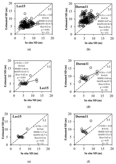
Figure 4.
Comparison of in situ measured SD values and MERIS-derived SD values: (a) using the Lee15 algorithm for all available in situ SD measurements; (b) using the Doron11 for all available in situ SD measurements; (c) using the Lee15 for matchups on the same day; (d) using the Doron11 for matchups on the same day; (e) using the Lee15 for matchups within 3 h; (f) using the Doron11 for matchups within 3 h.
Second, we compared in situ measured and MERIS data estimated SD values only for the same day matchups to reduce effects due to dynamic variation of water quality (Figure 4c,d, N = 23). Results revealed that RMSE and MAPE values were reduced to 1.86 m and 21.01% using the Lee15 algorithm, and 3.68 m and 66.87% with the Doron11 algorithm. In addition, the correlation coefficients were increased to 0.63 for the Lee15 algorithm and 0.65 for the Doron11 algorithm (p < 0.001). In this comparison, the Lee15 algorithm outperformed the Doron11 algorithm.
Third, we further compared in situ measured and MERIS-derived SD values for matchups with a time gap smaller than 3 h by considering NASA’s recommendation [37] and the high dynamic variation of water quality in the southeast arm of Lake Malawi (Figure 4e,f, N = 12). Results showed that the RMSE and MAPE values were further reduced to 1.17 m and 18.7% for Lee15 algorithm, with a correlation coefficient of 0.66 (p < 0.05) and slope of 0.74. However, the RMSE and MAPE values using Doron11 algorithm were slightly increased with an insignificant correlation between the measured and estimated SD values (R = 0.52 but p > 0.05). This comparison also demonstrated that the Lee15 algorithm performed better than the Doron11 algorithm.
Figure 5 presents an example of comparison of the MERIS-derived SD values using the Doron11 algorithm and Lee15 algorithm; a summary of the values during the study period is shown in Table 4 and Table 5. From Figure 5, it can be seen that the SD values derived by using the Doron11 algorithm were strongly correlated with those derived by using the Lee15 algorithm (nonlinear), but always with higher SD values for both yearly and monthly comparisons. Similar relationships could also be found for other years and months, with high determination coefficients larger than 0.96, absolute mean differences (AMD) ranging from 4.9–6.5 m, and relative mean differences (RMD) ranging from 37–58.7% (Table 4 and Table 5).
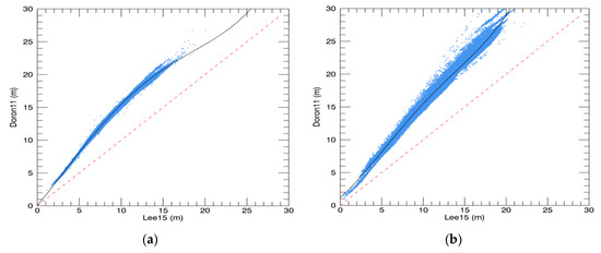
Figure 5.
Pixel-based comparison of MERIS-derived SD values using Doron11 algorithm and Lee15 algorithm in Lake Malawi. (a) yearly SD values in 2003; (b) monthly SD values for January.
Table 4.
Summary of pixel-based comparison of yearly MERIS-derived SD values using the Doron11 and Lee15 algorithms in Lake Malawi during the study period. The absolute mean difference (AMD) is calculated as averaged |Doron11_SD – Lee15_SD|, and the relative mean difference (RMD) is calculated as averaged |Doron11_SD – Lee15_ SD|/ Lee15_ SD × 100.
Table 5.
Summary of pixel-based comparison of monthly MERIS-derived SD values using the Doron11 algorithm and those using Lee15 algorithms in Lake Malawi during the study period. The absolute mean difference (AMD) is calculated as averaged |Doron11_SD – Lee15_SD|, and the relative mean difference (RMD) is calculated as averaged |Doron11_SD – Lee15_SD|/ Lee15_SD × 100.
3.2. Evaluation of Water Transparency in Lake Malawi
Figure 6 shows yearly water transparency level maps in Lake Malawi, which were generated from yearly SD distribution maps (obtained from MERIS data using the Lee15 algorithm) based on the OECD classification system [36] (i.e., Table 3). The yearly percentages for each water transparency level are summarized in Table 6. From Figure 6 and Table 6, it can be seen that: (1) Lake Malawi maintained four transparency levels throughout the period 2003–2011; (2) waters with transparency level 1 accounted for the largest area in the lake (58.7–79.7%), followed by waters with transparency level 2 (17.3–37.5%) and level 3 (2.2–3.6%), and with transparency level 4 (0.1–0.4%); (3) waters with transparency levels 3 and 4 were always distributed along the southwestern and southern lakeshores, and sometimes found in northern part (e.g., in 2004); (4) the largest change of transparency levels was found between levels 1 and 2; and (5) waters with transparency levels 1 and 2 accounted for more than 95% of the lake.
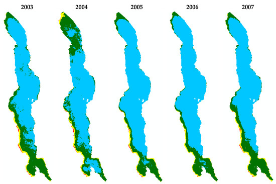
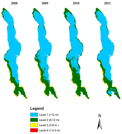
Figure 6.
Yearly water transparency level maps in Lake Malawi. These maps were generated from yearly SD distribution maps (obtained from MERIS data using the Lee15 algorithm) based on the Economic Cooperation and Development (OECD) classification system [36].
Table 6.
Yearly percentage for each water transparency level shown in (Figure 6).
Figure 7 shows monthly water transparency level maps in Lake Malawi, which were generated from monthly SD distribution maps (obtained from MERIS data using the Lee15 algorithm) based on the OECD classification system [36]. The monthly percentages for each water transparency level are summarized in Table 7. From Figure 7 and Table 7, it can be seen that there were several noticeable seasonal variations of SD in Lake Malawi. First, SD values from October–January were generally higher than in other months, and more than 78.5% of the water area was classified as transparency level 1 during the period. Second, the lake water was more turbid in February, April, July, and August than in other months due to water areas with transparency level 2 constituting more than 31.3% in these months; July, in particular, was dominated by water transparency level 2 (59.4%). Third, Lake Malawi was dominated by transparency levels 1 and 2 throughout the year (more than 95%), but the other two water transparency levels (i.e., levels 3 and 4) were also found in the lake each month.
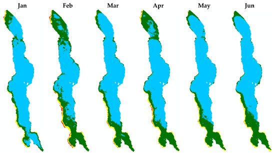
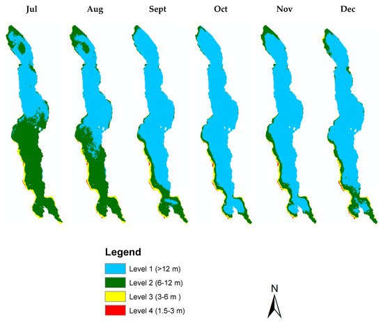
Figure 7.
Monthly water transparency level maps in Lake Malawi. These maps were generated from monthly SD distribution maps (obtained from MERIS data using the Lee15 algorithm) based on the OECD classification system [36].
Table 7.
Monthly percentage for each water transparency level shown in (Figure 7).
Figure 8 shows yearly averaged SD values in Lake Malawi from 2003 to 2011. Although a slightly decreased trend of SD values was observed, the change was not significant in Lake Malawi during the nine years (R2 = 0.051; p > 0.05). The highest and lowest yearly averaged SD values were observed in Lake Malawi in 2006 (13.6 m) and 2010 (11.6 m), respectively.
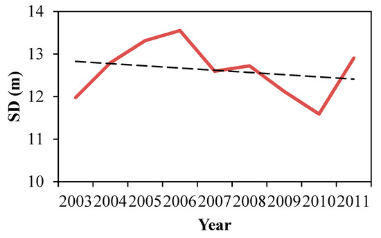
Figure 8.
Yearly averaged SD from 2003–2011 in Lake Malawi (red solid line); the black dashed (---) line represents the trend line.
4. Discussion
In this study, we compared two semi-analytical algorithms (i.e., Doron11 and Lee15) by applying them to Lake Malawi to estimate SD values from nine years of MERIS data (2003–2011). We found that although the two algorithms were developed based on different underwater visibility theories (i.e., classic and new), SD estimations using the two algorithms were highly correlated, with R2 larger than 0.96 (Figure 5; Table 4 and Table 5). Lee et al. [20] also reported a high R2 value of 0.89 when comparing the performance of the two algorithms with simulation data. These results indicate that there is no substantial difference between the two algorithms, especially if only one is used to evaluate water transparency change in a waterbody.
However, we found that the Doron11 algorithm always gave higher SD estimations than the Lee15 algorithm, with an averaged AMD value of 5.8 m in Lake Malawi. A similar trend was also found by Lee et al. [20]. In addition, by comparing the SD estimations from the two algorithms to in situ SD measurements, we found that the Lee15 algorithm outperformed the Doron11 algorithm with a MAPE value of 18.7% (Figure 4e). In contrast, the Doron11 algorithm overestimated SD values with a MAPE value of 73.4% (Figure 4f). These findings indicate that water quality would probably be overestimated if one used SD values from the Doron11 algorithm. For example, if we used SD distribution maps generated using the Doron11 to classify water transparency levels, we would have found that on average more than 94% of Lake Malawi was classified as level 1, and the sum of levels 3 and 4 would be less than 1% (results not shown).
Preisendorfer [31] reported that the value of the numerator of Equation (1) (i.e., Γ) could vary from 5 to 10. In the present study, the values of Γ were calculated in a range of 7.5–8.3, with an average of 7.9, within the range of initially published values. Therefore, we consider that the overestimations of SD values by Doron11 mainly derived from the denominator of Equation (1) (i.e., + ). Previous studies have pointed out that it is difficult to directly estimate from Rrs because of the ratio’s requirement of the backscattering and scattering coefficients, which cannot be obtained from Rrs [32]. In addition, it is well known that the ratio of the backscattering and scattering coefficients can vary temporally and spatially [32,38,39,40]. The Lee15 algorithm overcomes this difficulty, because the algorithm requires only . Therefore, Lee15 algorithm can be considered more robust than the Doron11 algorithm. However, we still found some overestimations in lower SD values and underestimations in higher SD values with the Lee15 algorithm (Figure 4), indicating that further improvements of the algorithm are necessary.
As mentioned in the introduction, there is no routine monitoring of water transparency in Lake Malawi due to the financial and institutional constraints in the surrounding countries [6]. In addition, even though there have been several studies measuring SD values by field surveys, it is difficult to use these measurements to evaluate water transparency or its changes for the entire lake, because all of these studies focused on only a small part of the lake for a short period of time. For example, Gondwe [41] investigated seasonal variation of SD in the Southeast Arm of Lake Malawi (see Figure 3 here) and reported that SD values ranged from 2.1 to 12.3 m; however, 79% of the SD values were between 4 and 8 m. Later, Macuiane et al. [42] reported that SD values were between 2 and 6 m in the Southeast part of the lake in 2012. In addition, Weyl et al. [22] reported that SD values were between 12 and 20 m in Lake Malawi.
None of the previous studies could show water transparency status for the entire surface of Lake Malawi, which, based on our results, always has four transparency levels (SD values ranging from 1.5 m to >12 m). The SD distribution maps generated from MERIS data can show not only the different water transparency levels, and the percentage and spatial distribution of each level, but also their seasonal and annual variations (Figure 6 and Figure 7). Such information is useful for lake water management. Therefore, we consider that the combination of satellite data and the semi-analytical algorithm (Lee15) to be a useful tool for routinely monitoring water quality in Lake Malawi.
Our results also showed that turbid waters (transparency levels 3 and 4) in Lake Malawi are mainly distributed along the southwestern lakeshore. This is probably because the majority of the inflowing rivers, population, and rainfall are concentrated in the southwestern watershed of the lake [43]. Although no significant water transparency changes were found in Lake Malawi during the study period (2003–2011), continuous monitoring of the lake’s water transparency remains necessary using Lee15 algorithm and more current new sensors such as Landsat 8/OLI, Sentinel-2/MSI, Sentinel-3/OLCI, which have been successfully used for deriving SD values in several previous studies [44,45,46].
Our future work will link the MERIS-derived SD values to trophic state of Lake Malawi. For this purpose, chlorophyll-a concentrations (Chl-a) in Lake Malawi are required to build a relationship between Chl-a and SD values as well as to determine coefficients for adapting Carlson’s trophic state index (CTSI, [18]) model [47,48,49,50]. Chl-a estimation from MERIS data is ongoing by using OC4E algorithm [51].
As pointed out by a previous study, loss of biodiversity due to fishing and nearshore water quality impacts has been a threat to Lake Malawi [52]. The information on water quality of Lake Malawi provided in this study can be used to help in the management of the lake and its basin as well as toward achieving the Sustainable Development Goal 6, target 6.3 (Monitoring Ambient Water Quality; [53]).
5. Conclusions
In this study, we first compared the performance of two semi-analytical algorithms (i.e., Doron11 and Lee15) in Lake Malawi. Our results showed that even though the SD estimations from the two algorithms were very highly correlated, with R2 larger than 0.96, the Lee15 algorithm outperformed the Doron11 algorithm in Lake Malawi with a high estimation accuracy (RMSE = 1.17 m, MAPE = 18.7%, R = 0.66, p < 0.05). The Doron11 usually overestimated SD values. These results indicate that water transparency in Lake Malawi can be evaluated by combining MERIS data and the Lee15 without algorithm recalibration using in situ data. This finding is important for most African lakes due to lack of in situ data for evaluating water quality or recalibrating an estimation algorithm in these lakes.
We then evaluated water transparency in Lake Malawi using the SD values estimated from nine years of MERIS data (2003–2011) with the Lee15 algorithm. Our results showed that there were always four water transparency levels in Lake Malawi throughout the study period. The levels 1 and 2 water areas tended to shift and trade places, depending on the year or season. In contrast, levels 3 and 4 water areas were relatively stable and constantly distributed along the southwestern and southern lakeshores. Generally, Lake Malawi is dominated by waters with SD values larger than 6 m (>95%). This is the first analysis to provide an overall and comprehensive assessment of water transparency status and spatiotemporal variation in Lake Malawi.
Author Contributions
A.V., B.M., D.J., F.S., T.F. took part in the development of the idea for the study and its conceptualization. D.J. and R.H. helped with the data processing. M.G. performed the field survey in Lake Malawi. A.V. performed data analysis, interpretation, and wrote the manuscript. B.M. supported the analysis and interpretation of the results, and revised and commented on the manuscript. F.S. and T.F. made substantial contribution to the design of the study.
Funding
This research was supported in part by the Grants-in-Aid for Scientific Research of MEXT from Japan (No. 17H01850 and No. 17H04475A).
Acknowledgments
The authors would like to show their gratitude to The Ministry of Education, Culture, Sports, Science, and Technology (MEXT) of Japan for the provision of the scholarship, the (ESA) Earth Observation Website for the MERIS L1B data, the BEAM ENVISAT for their free-of-charge Software. Their appreciation is extended to all Lab Members from the Water environment group in the Integrative Environment and Biomass Science Course. The authors would also like to thank two anonymous reviewers for their valuable comments and suggestions for improving the quality of the manuscript.
Conflicts of Interest
The authors declare no conflict of interest.
Appendix A
References
- Lehner, B.; Döll, P. Development and validation of a global database of lakes, reservoirs and wetlands. J. Hydrol. 2004, 296, 1–22. [Google Scholar] [CrossRef]
- Bootsma, H.A.; Hecky, R.E. Chapter 8: Nutrient Cycling in Lake Malawi/Nyasa. Available online: http://citeseerx.ist.psu.edu/viewdoc/download;jsessionid=5DC5D8129E0870AB9ED9C81219DAA9F6?doi=10.1.1.309.2651&rep=rep1&type=pdf (accessed on 22 January 2019).
- Snoeks, J. How well known is the ichthyodiversity of the large East African lakes? Adv. Ecol. Res. 2000, 31, 17–38. [Google Scholar]
- Hecky, R.E.; Bootsma, H.A.; Kingdon, M.L. Impact of Land Use on Sediment and Nutrient Yields to Lake Malawi/Nyasa (Africa). J. Great Lakes Res. 2003, 29 (Suppl. 2), 139–158. [Google Scholar] [CrossRef]
- Chavula, G.; Brezonik, P.; Thenkabail, P.; Johnson, T.; Bauer, M. Estimating chlorophyll concentration in Lake Malawi from MODIS satellite imagery. Phys. Chem. Earth 2009, 34, 755–760. [Google Scholar] [CrossRef]
- Ballatore, T.J.; Bradt, S.R.; Olaka, L.; Cózar, A.; Loiselle, S.A. Remote Sensing of African Lakes: A Review. In Remote Sensing of the African Seas; Barale, V., Gade, M., Eds.; Springer: Dordrecht, The Netherlands, 2014; Chapter 20; pp. 403–422. [Google Scholar]
- Dube, T.; Mutanga, O.; Seutloali, K.; Adelabu, S.; Shoko, C. Water Quality Monitoring in Sub-Saharan African Lakes: A Review of Remote Sensing Applications. Afr. J. Aquat. Sci. 2015, 40, 1–7. [Google Scholar] [CrossRef]
- IOCCG. Available online: http://ioccg.org/resources/missions-instruments/historical-ocean-colour-sensors/ (accessed on 3 October 2018).
- Mouw, C.B.; Greb, S.; Aurin, D.; Digiacomo, P.M.; Lee, Z.; Twardowski, M.; Binding, C.; Hu, C.; Ma, R.; Moore, T.; et al. Aquatic color radiometry remote sensing of coastal and inland waters: Challenges and recommendations for future satellite missions. Remote Sens. Environ. 2015, 160, 15–30. [Google Scholar] [CrossRef]
- Lee, Z.; Carder, K.L.; Arnone, R.A. Deriving inherent optical properties from water color: A multiband quasi-analytical algorithm for optically deep waters. Appl. Opt. 2002, 41, 5755–5772. [Google Scholar] [CrossRef]
- Lee, Z.P.; Shang, S.; Hu, C.; Du, K.P.; Weidemann, A.; Hou, W.; Lin, J.; Lin, G. Secchi disk depth: A new theory and mechanistic model for underwatervisibility. Remote Sens. Environ. 2015, 169, 139–149. [Google Scholar] [CrossRef]
- Gitelson, A.A.; Dall’Olmo, G.; Moses, W.; Rundquist, D.C.; Barrow, T.; Fisher, T.R.; Gurlin, D.; Holz, J. A simple semi-analytical model for remote estimation of chlorophyll-a in turbid waters: Validation. Remote Sens. Environ. 2008, 112, 3582–3593. [Google Scholar] [CrossRef]
- Gilerson, A.; Gitelson, A.; Zhou, J.; Gulrin, D.; Moses, W.; Ioannou, I.; Ahmed, S. Algorithms for remote sensing of chlorophyll-a in coastal and inland waters using red and near infrared bands. Opt. Express 2010, 18, 24109–24125. [Google Scholar] [CrossRef]
- Yang, W.; Matsushita, B.; Chen, J.; Fukushima, T. Estimating constituent concentrations in case II waters from MERIS satellite data by semi-analytical model optimizing and look-up tables. Remote Sens. Environ. 2011, 115, 1247–1259. [Google Scholar] [CrossRef]
- Nechad, B.; Ruddick, K.G.; Park, Y. Calibration and validation of a generic multisensor algorithm for mapping of total suspended matter in turbid waters. Remote Sens. Environ. 2010, 114, 854–866. [Google Scholar] [CrossRef]
- Doron, M.; Babin, M.; Hembise, O.; Mangin, A.; Garnesson, P. Ocean transparency from space: Validation of algorithms using MERIS, MODIS and SeaWiFS data. Remote Sens. Environ. 2011, 115, 2986–3001. [Google Scholar] [CrossRef]
- Secchi, P.A. Relazione delle esperienze fatte a bordo della pontificia pirocorvetta Imacolata Concezione per determinare la trasparenza del mare. In Il Nuovo Cimento Giornale de Fisica, Chimica e Storia Naturale; G.B. Paravia: Torino, Italy, 1864; Volume 20, pp. 205–237. [Google Scholar]
- Carlson, R.E. A trophic state index for lakes. Limnol. Oceanogr. 1977, 22, 361–369. [Google Scholar] [CrossRef]
- Duntley, S.Q. The Visibility of Submerged Objects; Visibility Lab. Mass. Inst. Tech.: San Diego, CA, USA, 1952; 74p. [Google Scholar]
- Lee, Z.; Shang, S.; Du, K.; Wei, J. Resolving the long-standing puzzles about the observed Secchi depth relations. Limnol. Oceanogr. 2018, 63, 2321–2336. [Google Scholar] [CrossRef]
- Odermatt, D.; Danne, O.; Philipson, P.; Brockmann, C. Diversity II water quality parameters for 300 lakes worldwide from ENVISAT (2002–2012). Earth Syst. Sci. Data 2018, 10, 1527–1549. [Google Scholar] [CrossRef]
- Weyl, O.L.F.; Ribbink, A.J.; Tweddle, D. Lake Malawi: Fishes, fisheries, biodiversity, health and habitat. Aquat. Ecosyst. Health Manag. 2010, 13, 241–254. [Google Scholar] [CrossRef]
- Bootsma, H.; Jorgensen, S.E. Lake Malawi/Nyasa. In Managing Lake Basins: Practical Approaches for Sustainable Use; Nakamura, M., Ed.; ILEC Foundation: Kusatsu, Japan, 2004; 36p, Available online: www.worldlakes.org/uploads/ELLB%20Malawi-NyasaDraftFinal.14Nov2004.pdf (accessed on 16 September 2017).
- World Bank Climate Portal. Available online: http://sdwebx.worldbank.org/climateportal (accessed on 19 June 2017).
- MERCI. Available online: http://merisfrs-merci-ds.eo.esa.int/merci (accessed on 17 March 2016).
- Doerffer, R.; Schiller, H. Algorithm Theoretical Basis Document (ATBD). MERIS Regional Coastal and Lake Case 2 Water Project Atmospheric Correction ATBD; GKSS Research Center: Geesthacht, Germany, 2008. [Google Scholar]
- Koponen, S.; Ruiz-Verdu, A.; Heege, T.; Heblinski, J.; Sorensen, K.; Kallio, K.; Pyhälahti, T.; Doerffer, R.; Brockmann, C.; Peters, M. Development of MERIS Lake Water Algorithms: Validation Report; ESRIN: Frascati, Italy, 2008. [Google Scholar]
- Doerffer, R.; Brockmann, C. Consensus Case 2 Regional Algorithm Protocols; Technical Report; Brockmann Consult: Geesthacht, Germany, 2014. [Google Scholar]
- Gondwe, M.J.S.; Guildford, S.J.; Hecky, R.E. Physical-chemical measurements in the water column along a transect through a tilapia cage fish farm in Lake Malawi, Africa. J. Great Lakes Res. 2011, 37, 102–113. [Google Scholar] [CrossRef]
- Tyler, J.E. The secchi disc. Limnology and oceanography. Limnol. Oceanogr. 1968, 13, 1–6. [Google Scholar] [CrossRef]
- Preisendorfer, R.W. Secchi disk science: Visual optics of natural waters. Limnol. Oceanogr. 1986, 31, 909–926. [Google Scholar] [CrossRef]
- Doron, M.; Babin, M.; Mangin, A.; Hembise, O. Estimation of light penetration, and horizontal and vertical visibility in oceanic and coastal waters from surface reflectance. J. Geophys. Res. 2007, 112, C06003. [Google Scholar] [CrossRef]
- Lee, Z.P.; Hu, C.; Shang, S.; Du, K.; Lewis, M.; Arnone, R.; Brewin, R. Penetration of UV–visible solar light in the global oceans: Insights from ocean color remote sensing. J. Geophys. Res. 2013, 118, 4241–4255. [Google Scholar] [CrossRef]
- Zhang, X.; Hu, L.; He, M.X. Scattering by pure seawater: Effect of salinity. Opt. Express 2009, 17, 5698–5710. [Google Scholar] [CrossRef] [PubMed]
- International Ocean-Colour Coordinating Group (IOCCG_QAA_v6, 2014). Available online: http://www.ioccg.org/groups/software.html (accessed on 20 May 2017).
- OECD. Eutrophication of Waters: Monitoring, Assessment and Control; Technical Report; Environmental Directorate, OECD: Paris, France, 1982; p. 147. [Google Scholar]
- Bailey, S.W.; Werdell, P.J. A multi-sensor approach for the on-orbit validation of ocean color satellite data products. Remote Sens. Environ. 2006, 102, 12–23. [Google Scholar] [CrossRef]
- Twardowski, M.S.; Boss, E.; Macdonald, J.B.; Pegau, W.S.; Barnard, A.H.; Zaneveld, J.R.V. A model for estimating bulk refractive index from the optical backscattering ratio and the implications for understanding particle composition in case I and case II waters. J. Geophys. Res. Oceans 2001, 106, 14129–14142. [Google Scholar] [CrossRef]
- Loisel, H.; Meriaux, X.; Berthon, J.F.; Poteau, A. Investigation of the optical backscattering to scattering ratio of marine particles in relation to their biogeochemical composition in the eastern English Channel and southern North Sea. Limnol. Oceanogr. 2007, 52, 739–752. [Google Scholar] [CrossRef]
- Stramska, M.; Stramski, D.; Mitchell, B.G.; Mobley, C.D. Estimation of the absorption and backscattering coefficients from in-water radiometric measurements. Limnol. Oceanogr. 2000, 45, 628–641. [Google Scholar] [CrossRef]
- Gondwe, M.J.G.S. Environmental Impacts of Cage Aquaculture in the Southeast Arm of Lake Malawi: Water and Sediment Quality and Food Web Changes. Ph.D. Thesis, University of Waterloo, Waterloo, ON, Canada, 2009. [Google Scholar]
- Macuiane, M.; Hecky, R.; Guildford, S. Temporal and Spatial Changes in Water Quality in Lake Malawi/Niassa, Africa: Implications for Cage Aquaculture Management. Ocean Fish. Open Access J. 2016, 1, 555552. [Google Scholar]
- Nicholson, S.E.; Klotter, D.; Chavula, G. A detailed rainfall climatology for Malawi, Southern Africa. Int. J. Climatol. 2014, 34, 315–325. [Google Scholar] [CrossRef]
- Lee, Z.; Shang, S.; Qi, L.; Yan, J.; Lin, G. A semi-analytical scheme to estimate Secchi- disk depth from Landsat-8 measurements. Remote Sens. Environ. 2016, 177, 101–106. [Google Scholar] [CrossRef]
- Rodrigues, T.; Alcântara, E.; Watanabe, F.; Imai, N. Retrieval of Secchi disk depth from a reservoir using a semi-analytical scheme. Remote Sens. Environ. 2017, 198, 213–228. [Google Scholar] [CrossRef]
- Toming, K.; Kutser, T.; Uiboupin, R.; Arikas, A.; Vahter, K.; Paavel, B. Mapping water quality parameters with Sentinel-3 Ocean and Land Colour Instrument imagery in the Baltic Sea. Remote Sens. 2017, 9, 1070. [Google Scholar] [CrossRef]
- Cheng, K.S.; Lei, T.C. Reservoir Trophic State Evaluation using Landsat TM Images. J. Am. Water Resour. Assoc. 2001, 37, 1321–1334. [Google Scholar] [CrossRef]
- Cunha, D.G.F.; Ogura, A.P.; Calijuri, M.C. Nutrient reference concentrations and trophic state in subtropical reservoirs. Water Sci. Technol. 2012, 65, 1461–1467. [Google Scholar] [CrossRef] [PubMed]
- Sheela, A.M.; Letha, J.; Joseph, S.; Ramachandra, K.K.; Sanalkumar, S.P. Trophic state index of a lake system using IRS (P6-LISS III) satellite imagery. Environ. Monit. Assess. 2011, 177, 575–592. [Google Scholar] [CrossRef] [PubMed]
- Membrillo-Abad, A.S.; Torres-Vera, M.A.; Alcocer, J.; Prol-Ledesma, R.M.; Oseguera, L.A.; Ruiz-Armenta, J.R. Trophic State Index estimation from remote sensing of lake Chapala, Mexico. Revista Mexicana de Ciencias Geologicas. 2016, 33, 183–191. [Google Scholar]
- O’Reilly, J.E.; Maritorena, S.; Mitchell, B.G.; Siegel, D.A.; Carder, K.L.; Garver, S.A.; Kahru, M.; Mcclain, C. Ocean color chlorophyll algorithms for SeaWiFS. J. Geophys. Res. 1998, 103, 937–953. [Google Scholar] [CrossRef]
- Bootsma, H.A.; Jorgensen, S.E. Lake Malawi/Nyasa. Experiences and Lessons Learned Brief. Available online: http://www.worldlakes.org/uploads/16_lake_malawi_nyasa_27february2006.pdf (accessed on 21 January 2019).
- United Nations Open Working Group 2014—Monitoring Ambient Water Quality. Available online: http://www.sdg6monitoring.org/indicators/target-63/indicators632/ (accessed on 22 January 2019).
© 2019 by the authors. Licensee MDPI, Basel, Switzerland. This article is an open access article distributed under the terms and conditions of the Creative Commons Attribution (CC BY) license (http://creativecommons.org/licenses/by/4.0/).