Improved Faraday Rotation Estimation in Spaceborne PolSAR Data Using Total Variation Denoising

Abstract

Faraday rotation (FR) is a serious problem for spaceborne polarization SAR (PolSAR) systems at L and P bands. One way to solve the problem is to estimate the FR from PolSAR data for further compensation. Therefore, precise estimation of FR from PolSAR data not only determines the compensation effect of polarimetric systems but also benefits the ionospheric sounding with high spatial resolution. Among the factors that affect the FR estimation, system noise is a non-neglectable factor. Although average filtering (AF) has been widely used in previous works for noise removing it depends on large window size, and therefore reduces the spatial resolution of FR estimation. In order to realize optimal noise suppression with minimized resolution loss, the total variation (TV) denoising method is applied in this paper. By testing the Advanced Land Observing Satellite (ALOS) Phased Array L-band Synthetic Aperture Radar (PALSAR) full-pol datasets, TV and AF are compared and validated. Results using synthetic and real data show that, after TV denoising, the FR can be recovered with high spatial resolution and the noise level in estimated FR is reduced more effectively than that after AF.

1. Introduction

The ionosphere, a crucial component of the space environment, is mainly distributed over the earth at an altitude of 60 to 1000 km. Given the presence of a large number of free electrons in the ionosphere and the presence of an ambient geomagnetic field, the polarization of spaceborne radar signals at L-band or lower frequencies is changed when the signals pass through the ionosphere. The changing of polarization is called Faraday rotation (FR). FR error, therefore, deteriorates the quality of the scattering matrix and decreases the performance of the polarimetric radar system [1,2]. To address this issue, research on detecting and correcting FR is crucial. However, distorted echoes contain abundant ionospheric information. The ionospheric sounding based on the PolSAR system is possible if the mechanisms of ionospheric interference are understood and accurately modeled [3,4]. In this way, both Earth observation and ionospheric sounding could be done in one spaceborne SAR mission, thus reducing the cost.

Plenty of methods have been proposed to estimate FR from PolSAR data. In accordance with the full-polarization (full-pol) SAR data treatment, several classical FR estimators are introduced here. After transforming the scatter matrix from Cartesian linear polarization to circular polarization, Bickel and Bates proposed a widely used FR estimator [5]. Freeman converted the scattering matrix to the covariance matrix. By measuring the covariance matrix, Freeman proposed several FR estimators [6]. Chen and Quegan further proposed a FR estimator based on the off-diagonal terms of covariance matrix [7]. We also proposed a new FR estimator using the covariance matrix of circle basis [8]. Although many estimators are available today, none of them perfectly resist the influence of system errors. Fortunately, for the Advanced Land Observing Satellite (ALOS) Phased Array L-band Synthetic Aperture Radar (PALSAR), the channel imbalance and crosstalk of the system are well calibrated by the Japan Aerospace Exploration Agency (JAXA) [9,10]. Therefore, in most cases, the system noise is the only factor that influences the precision of FR estimation.

In previous studies, the system noise is usually suppressed by average filtering (AF). One inherent problem of AF is that the precision and resolution of filtered signals are restricted by the size of the filtering window. Increasing the window size also increases the precision but simultaneously decreases the spatial resolution, and vice versa. The relationship between the precision and the window size has been emphasized in [11]. In order to simultaneously improve the precision and resolution of estimated FR image, a denoising method called total variation (TV) [12] is applied in this paper. TV denoising is capable of keeping the edges of an image while suppressing random Gaussian noise, thus, improving the FR precision without loss of spatial resolution.

The outline of this paper is as follows: In Section 2, the method for FR estimation from PolSAR data is briefly reviewed and based on it, the theory of TV denoising is proposed. Then, in Section 3 synthetic and real experiments are conducted to validate the ability of TV to keep both the precision and spatial resolution of estimated FR images. Results on five different PolSAR scenes prove the effectiveness of the TV method. Finally, our conclusions are outlined in Section 4.

2. Materials and Methods

2.1. FR Estimation

The spaceborne SAR signals suffer from FR effects during their propagation through the ionosphere. If the radar system is well calibrated, the actual measured scattering matrix $M$ will be related with the true scattering matrix $S$ as:

$$\left[\begin{array}{cc}{M}_{hh}& M_{vh}\\ M_{hv}& M_{vv}\end{array}\right]=\left[\begin{array}{cc}\cos \mathsf{\Omega }& \sin \mathsf{\Omega }\\ -\sin \mathsf{\Omega }& \cos \mathsf{\Omega }\end{array}\right]\left[\begin{array}{cc}{S}_{hh}& S_{vh}\\ S_{hv}& S_{vv}\end{array}\right]\left[\begin{array}{cc}\cos \mathsf{\Omega }& \sin \mathsf{\Omega }\\ -\sin \mathsf{\Omega }& \cos \mathsf{\Omega }\end{array}\right]+\left[\begin{array}{cc}{N}_{hh}& N_{vh}\\ N_{hv}& N_{vv}\end{array}\right],$$

(1)

where $N$ matrix is the system noise and $\mathsf{\Omega }$ denotes the FR angle. According to Equation (1), many methods for FR retrieval have been developed [5,6,7,8,13,14]. In this work, the B&B method is selected as a reference due to its well-known robustness [15,16].

The B&B method first transforms $M$ from Cartesian linear polarization to circular polarization:

$$\left[\begin{array}{cc}{Z}_{11}& Z_{12}\\ Z_{21}& Z_{22}\end{array}\right]=\left[\begin{array}{cc}1& j\\ j& 1\end{array}\right]\left[\begin{array}{cc}{M}_{hh}& M_{vh}\\ M_{hv}& M_{vv}\end{array}\right]\left[\begin{array}{cc}1& j\\ j& 1\end{array}\right]$$

(2)

Then, Equation (1) is substituted into Equation (2) to give:

$$Z_{12}{Z}_{21}^{\ast }=\left(S_{hh}+S_{vv}\right)\exp \left(-i4\mathsf{\Omega }\right)+\tilde{N}.$$

(3)

where $\tilde{N}$ is a Gaussian noise component brought in by $N$. If the noise $\tilde{N}$ is well filtered, then FR angle could be simply estimated as:

$$\mathsf{\Omega }=-\frac{1}{4}\arg \left(Z_{12}{Z}_{21}^{\ast }\right).$$

(4)

If the system noise is considered, the B&B method becomes [5]:

$$\mathsf{\Omega }=-\frac{1}{4}\arg \left(\langle Z_{12}{Z}_{21}^{\ast }\rangle \right),$$

(5)

where $\langle \cdot \rangle$ is a function of average filtering (AF). This method could retrieve the FR with high precision if a large filtering window is adopted. However, the larger the filtering window is, the lower the space resolution of FR is [11]. To obtain FR with high precision and high resolution, another denoising method is needed. Therefore, in this paper we introduce TV denoising.

2.2. TV Denoising

TV denoising is a famous denoising method in the image process area [17,18,19,20]. The principle of TV denoising is to remove the noise while keeping the image edges, so it will keep the sharpness in the image, thus, keeping the spatial resolution.

For image $I$ that suffered from noise $N$, we want to reconstruct the true image $T$ from $I$:

$$I=T+N$$

(6)

This problem has been studied for decades [12,21,22,23]. One popular technique for this reconstruction belongs to Rudin, Osher, and Fatemi [21], and can be expressed as an optimization problem:

$$T=\underset{T}{\arg \min }\left\{\left|{\nabla }_{x}T\right|+\left|{\nabla }_{y}T\right|+\frac{\mu }{2}{\Vert I-T\Vert }_2^2\right\}$$

(7)

where $\mu$ is a scale parameter to control the approximation of $I$ to $T$. Several methods have been proposed to solve this problem [12,21,22,23]. Among them, in this paper, the split Bregman method [12] is chosen for its efficiency.

The split Bregman method is designed to solve the class of $l_1$-regularized optimization problems. The major advantage is that the split Bregman method decouples the objective function, i.e., Equation (7) into $l_1$ and $l_2$ portions, thus facilitating the optimization process. This method first rewrites Equation (7) as a constrained problem:

$$\underset{T,d_x,d_y}{\min }\left|d_x\right|+\left|d_y\right|+\frac{\mu }{2}{\Vert I-T\Vert }_2^2$$

(8)

where $d_x=\left|{\nabla }_{x}T\right|$ and $d_y=\left|{\nabla }_{y}T\right|$. Then the constrained problem could be rearranged as an unconstrained one by adding penalty function terms

$$\underset{T,d_x,d_y}{\min }\left|d_x\right|+\left|d_y\right|+\frac{\mu }{2}{\Vert I-T\Vert }_2^2+\frac{\lambda }{2}{\Vert d_x-{\nabla }_{x}T\Vert }_2^2+\frac{\lambda }{2}{\Vert d_y-{\nabla }_{y}T\Vert }_2^2$$

(9)

In this way, Equation (7) could be solved by adopting Bregman iteration [24], which leads to

$$\left(T^{k+1},d_x^{k+1},d_y^{k+1}\right)=\underset{T,d_x,d_y}{\min }\left|d_x^k\right|+\left|d_y^k\right|+\frac{\mu }{2}{\Vert I-T^k\Vert }_2^2+\frac{\lambda }{2}{\Vert d_x^k-{\nabla }_x{T}^k-b_x^k\Vert }_2^2+\frac{\lambda }{2}{\Vert d_y^k-{\nabla }_y{T}^k-b_y^k\Vert }_2^2$$

(10)

where

$$\begin{array}{c}{b}_x^{k+1}=b_x^k+\left({\nabla }_x{T}^{k+1}-d_x^{k+1}\right)\\ b_y^{k+1}=b_y^k+\left({\nabla }_y{T}^{k+1}-d_y^{k+1}\right)\end{array}$$

(11)

Therefore, the original optimization problem Equation (7) is now turned into an iterative minimization problem consisting of Equation (10) and Equation (11). According to the work of [12], Equation (10) could be solved by splitting it into $l_1$ component and $l_2$ component:

$$T^{k+1}=\underset{T}{\min }\frac{\mu }{2}{\Vert T^k-I\Vert }_2^2+\frac{\lambda }{2}{\Vert d_x^k-{\nabla }_x{T}^k-b_x^k\Vert }_2^2+\frac{\lambda }{2}{\Vert d_y^k-{\nabla }_y{T}^k-b_y^k\Vert }_2^2$$

(12)

and

$$\begin{array}{c}{d}_x^{k+1}=\underset{d}{\min }\left|d_x\right|+\frac{\lambda }{2}{\Vert d-{\nabla }_x{T}^{k+1}-b_x^k\Vert }_2^2\\ d_y^{k+1}=\underset{d}{\min }\left|d_y\right|+\frac{\lambda }{2}\Vert d-{\nabla }_y{T}^{k+1}-b_y^k\Vert \end{array}$$

(13)

By now, Equation (12) becomes differentiable and can be solved using the Gauss–Seidel method

$$T_{i,j}^{k+1}=\frac{\lambda }{\mu +4\lambda }\left(\begin{array}{l}{T}_{i+1,j}^k+T_{i-1,j}^k+T_{i,j+1}^k+T_{i,j-1}^k+d_{x,i-1,j}^k-d_{x,i,j}^k+d_{y,i,j-1}^k\\ -d_{y,i,j}^k-b_{x,i-1,j}^k+b_{x,i,j}^k-b_{y,i,j-1}^k+b_{y,i,j}^k\end{array}\right)+\frac{\lambda }{\mu +4\lambda }{I}_{i,j}$$

(14)

The subscripts $i$ and $j$ in Equation (14) are the pixel coordinates of an image. Equation (13) can be explicitly solved using shrinkage operators:

$$\begin{array}{l}{d}_x^{k+1}=shrink\left({\nabla }_x{u}^{k+1}+b_x^k,1/\lambda \right)\\ d_y^{k+1}=shrink\left({\nabla }_y{u}^{k+1}+b_y^k,1/\lambda \right)\end{array}$$

(15)

and the $shrink$ function is defined as:

$$shrink\left(x,y\right)=\frac{x}{\left|x\right|}\max \left(\left|x\right|-y,0\right)$$

(16)

For more details about the split Bregman method, refer to [12].

Comparing Equation (3) to Equation (6) we will find that $Z_{12}{Z}_{21}^{\ast }$ is corresponding to $I$ and that the real image $T$ corresponds to $\left(S_{hh}+S_{vv}\right)\exp \left(-i4\mathsf{\Omega }\right)$. Therefore, the whole process for denoising $Z_{12}{Z}_{21}^{\ast }$ is summarized in

Table 1. The process for $Z_{12}{Z}_{21}^{\ast }$ denoising.

Calculate the $Z_{12}{Z}_{21}^{\ast }$ of each scene according to Equation (2).

Let $T^0=I=Z_{12}{Z}_{21}^{\ast }$, and $d_x^0=d_y^0=b_x^0=b_y^0=0$.

Define the maximum number of iterations as $threshold$,

and initial the number of iterations $k=0$.

While ${\Vert T^k-T^{k-1}\Vert }_2>tol$ and $k<threshold$

Calculate $T^k$ from Equation (14),

update $d_x$,$d_y$ using Equation (15),

update $b_x$,$b_y$ with Equation (11),

update the number of iterations $k=k+1$.

end

.

Resulting $T^k$ from Table 1 is exactly the denoised $Z_{12}{Z}_{21}^{\ast }$, then Equation (4) could be used for FR retrieval.

3. Experimental Results and Discussion

To evaluate the performance of the TV denoising method, both synthetic and real experiments are conducted.

3.1. Synthetic Experiment

In the synthetic experiment, two PolSAR scenes are randomly chosen from the PALSAR dataset [25]. The data information is given in

Table 2. Details of two PolSAR scenes used for synthetic experiment.

Scene No.	Locations	Observation Time
Scene 1	(56.456N, -161.598W)	20110328 08:41
Scene 2	(49.578N, 118.250E)	20070428 14:13

. For each scene, first, we make sure the PolSAR data is reciprocal by:

$$S_{hv}=S_{vh}=\left(S_{hv}+S_{vh}\right)/2,$$

(17)

Therefore, known FR and Gaussian noise can be added to each scene according to Equation (1).

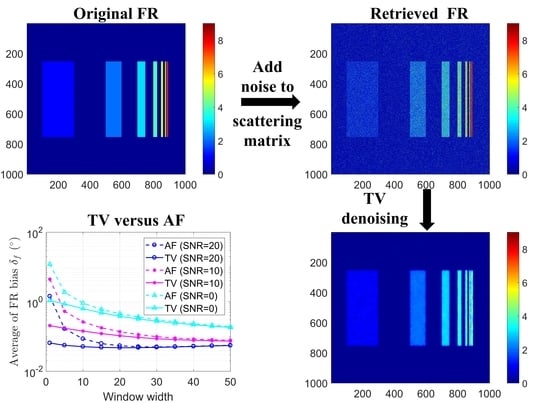
The FR images used as ground truth are given in Figure 1. Figure 1a is retrieved from an unrelated PolSAR scene using the B&B method to test the TV algorithm on real FR data, and Figure 1b is constructed manually. There are nine slices of FR in Figure 1b with values increasing from $1^{\circ }$ to $9^{\circ }$ and widths decreasing from 200 pixels to 1 pixels. The background of Figure 1b is set to be zero. Using Figure 1b, the performance of TV in keeping spatial resolutions can be directly viewed.

To test the performance of the proposed method against different levels of noise, we add to the scene Gaussian noise under SNR = 0 dB, SNR = 10 dB, and SNR = 20 dB, respectively. The SNR is defined as [14]

$$SNR=10\lg \left(\frac{\langle S_{hh}{S}_{hh}^{\ast }\rangle +2\langle S_{hv}{S}_{hv}^{\ast }\rangle +\langle S_{vv}{S}_{vv}^{\ast }\rangle }{\langle {\left|N_{hh}\right|}^2\rangle +2\langle {\left|N_{hv}\right|}^2\rangle +\langle {\left|N_{vv}\right|}^2\rangle }\right).$$

(18)

In the experiment, the noise level of each channel is set to be equal [14]

$$\langle {\left|N_{hh}\right|}^2\rangle =\langle {\left|N_{vh}\right|}^2\rangle =\langle {\left|N_{hv}\right|}^2\rangle =\langle {\left|N_{vv}\right|}^2\rangle ,$$

(19)

Therefore, the standard deviation of noise in each channel is calculated as:

$${\delta }_N=\left(\frac{\langle S_{hh}{S}_{hh}^{\ast }\rangle +2\langle S_{hv}{S}_{hv}^{\ast }\rangle +\langle S_{vv}{S}_{vv}^{\ast }\rangle }{{10}^{SNR/10}\times 4}\right).$$

(20)

As the true FR is known, if the method could remove all the noise, the bias between estimated FR and the true value is zero. We compared TV with the traditional method, i.e., average filtering (AF). In the AF algorithm, the size of the filtering window plays an important role. A larger window suppresses the noise more, but it also decreases the FR resolution. Instead of using a fixed window, we test AF under a different number of looks [11] (the number of looks is defined as the number of pixels of the filtering window). In the experiment, all filtering windows are set to be square, that is to say, $225$ looks correspond to a $15\times 15$ window. Actually, during our test it is the number of looks that influences the result the most rather than the window shape. Therefore, if a $5\times 45$ window is used, the same result is obtained as using a $15\times 15$ window. Although the TV algorithm does not involve a filtering window, for a fair comparison we also added a filtering window after the TV algorithm was executed, that is to say, in the experiment below, the results of TV are obtained by first applying the TV algorithm and, then, adopting the AF algorithm. However, as described in the following, our main concern is the result of TV with a $1\times 1$ window, i.e., the result from a pure TV algorithm. Results with all other windows are used for a fair comparison with the AF method.

3.1.1. Result on the First FR Image

Figure 2 gives the result of two selected PolSAR scenes on the first FR image (shown in Figure 1a) under three levels of noise. The left column of Figure 2 shows the average of the FR bias ${\delta }_f$ of each scene changing with respect to different looks

$${\delta }_f=mean\left|{\mathsf{\Omega }}_E-{\mathsf{\Omega }}_T\right|$$

(21)

and the right column shows the standard deviation of the FR bias ${\sigma }_f$ in each scene

$${\sigma }_f=std\left|{\mathsf{\Omega }}_E-{\mathsf{\Omega }}_T\right|$$

(22)

In Equation (21) and Equation (22), ${\mathsf{\Omega }}_E$ and ${\mathsf{\Omega }}_T$ represent estimated the FR and the true FR, respectively. The closer the ${\delta }_f$ and ${\sigma }_f$ are to zero, the better the algorithm performs. For a better illustration of differences between the two methods, the logarithmic scale is used for the y-axis and the linear scale is used for the x-axis. Specifically, the coordinate of the x-axis denotes the width of the filtering window, i.e., the square root of the number of looks. As we can see from Figure 2, the bias of FR decreases as the SNR gets higher, but regardless of the noise level, the TV method performs much better than AF. For Scene 1, we find that the TV method with $1\times 1$ looks performs similar or even better than AF with $15\times 15$ looks in terms of both ${\delta }_f$ and ${\sigma }_f$, which means, in Scene 1, TV with $1\times 1$ looks could achieve the same noise removing performance as AF with $15\times 15$ looks.

For Scene 2, the superiority of TV in terms of ${\delta }_f$ is much more obvious. Specifically, the ${\delta }_f$ of TV with $1\times 1$ looks is smaller than that of AF with $30\times 30$ looks under the same noise level. However, the performance of TV in terms of ${\sigma }_f$ seems not satisfying. From Figure 2d we can find for SNR = 20 dB, the ${\sigma }_f$ of TV with $1\times 1$ looks is unexpectedly larger than that of AF with $15\times 15$ looks. Recalling that ${\sigma }_f$ means the standard deviation of FR bias, a larger ${\sigma }_f$ means the bias will spread in a wider range. Nevertheless, when we examine the distribution of FR bias of TV and AF, we find that the bias of TV with $1\times 1$ looks is still more centralized than the bias of AF with $15\times 15$ looks, as shown by the bias histograms in Figure 3. Obviously we can see from Figure 3 the FR bias of TV with $1\times 1$ looks (Figure 3b) is distributed more concentrated around zero than bias of AF with $15\times 15$ looks (Figure 3a). The larger ${\sigma }_f$ of TV with $1\times 1$ looks is mainly caused by a very few pixels whose values are abnormally large due to remaining noise. The number of abnormal pixels is so small (about 50 in a million) that they do not influence the image precision and resolution too much. Therefore, in Scene 2, TV with $1\times 1$ looks still performs better than AF with $15\times 15$ looks. In conclusion, TV could obtain FR in high precision as AF achieves with $15\times 15$ looks.

Another phenomenon is that the increase of the window width also reduces the bias of FR, which accords with the conclusion given in [11]. However, an interesting fact could be observed from both scenes under noise level SNR = 20 dB that the FR bias increases a little after it reaches to a minimum. This phenomenon is more obvious in TV than in AF. At first sight, it seems contradictory to the conclusions in [11]. However, the conclusions in [11] are based on the assumption that the FR angles adding to each pixel are equal. Recalling Equation (3) here, if the FR in each pixels is equal to each other, then a large window will suppress the noise only, but if the FR varies pixel by pixel, a large window will also distort the original FR in each pixel. For example, assume there is a FR image only consisting of two pixel, then according to Equation (3) we would get the two following equations to derive the FR of the two pixels:

$$Z_{12}{Z}_{21}^{\ast }=S_1\exp \left(-i4{\mathsf{\Omega }}_1\right)+{\tilde{N}}_1,$$

(23)

and

$$Z_{12}{Z}_{21}^{\ast }=S_2\exp \left(-i4{\mathsf{\Omega }}_2\right)+{\tilde{N}}_2.$$

(24)

To eliminate the noise, a 2 looks filtering window is assumed to be used, then, according to Equation (5) the derived FR would be

$$\mathsf{\Omega }=-\frac{1}{4}\arg (\frac{S_1\exp \left(-i4{\mathsf{\Omega }}_1\right)+S_2\exp \left(-i4{\mathsf{\Omega }}_2\right)}{2}+\frac{{\tilde{N}}_1+{\tilde{N}}_2}{2}).$$

(25)

From Equation (25) we can easily find that if ${\mathsf{\Omega }}_1={\mathsf{\Omega }}_2$, the precision of $\mathsf{\Omega }$ is only affected by the noise component. However when ${\mathsf{\Omega }}_1\ne {\mathsf{\Omega }}_2$, even if the noise is perfectly eliminated, resulting $\mathsf{\Omega }$ would still be biased by the difference between ${\mathsf{\Omega }}_1$ and ${\mathsf{\Omega }}_2$. This result explains why under SNR = 20 dB the resulting FR bias with a large window is larger than that with a small window. A large window suppressed the noise component well but suffers more from the FR variation. Therefore, in real scenes a large filtering window is not always a good option.

From Equation (25), we know if the noise is well removed, we will have

$$\left[\begin{array}{cc}{\widehat{S}}_{hh}& {\widehat{S}}_{vh}\\ {\widehat{S}}_{hv}& {\widehat{S}}_{vv}\end{array}\right]=\left[\begin{array}{cc}\cos {\mathsf{\Omega }}_E& -\sin {\mathsf{\Omega }}_E\\ \sin {\mathsf{\Omega }}_E& \cos {\mathsf{\Omega }}_E\end{array}\right]\left[\begin{array}{cc}{\widehat{M}}_{hh}& {\widehat{M}}_{vh}\\ {\widehat{M}}_{hv}& {\widehat{M}}_{vv}\end{array}\right]\left[\begin{array}{cc}\cos {\mathsf{\Omega }}_E& \sin {\mathsf{\Omega }}_E\\ -\sin {\mathsf{\Omega }}_E& \cos {\mathsf{\Omega }}_E\end{array}\right]$$

(26)

where the $\widehat{M}$ matrix is the noise free scattering matrix that could be calculated in the synthetic experiment as:

$$\left[\begin{array}{cc}{\widehat{M}}_{hh}& {\widehat{M}}_{vh}\\ {\widehat{M}}_{hv}& {\widehat{M}}_{vv}\end{array}\right]=\left[\begin{array}{cc}\cos {\mathsf{\Omega }}_T& \sin {\mathsf{\Omega }}_T\\ -\sin {\mathsf{\Omega }}_T& \cos {\mathsf{\Omega }}_T\end{array}\right]\left[\begin{array}{cc}{S}_{hh}& S_{vh}\\ S_{hv}& S_{vv}\end{array}\right]\left[\begin{array}{cc}\cos {\mathsf{\Omega }}_T& \sin {\mathsf{\Omega }}_T\\ -\sin {\mathsf{\Omega }}_T& \cos {\mathsf{\Omega }}_T\end{array}\right]$$

(27)

When FR is precisely estimated, the resulting ${\widehat{S}}_{vh}$ and ${\widehat{S}}_{hv}$ from Equation (26) will be reciprocal, that is to say the differences between ${\widehat{S}}_{vh}$ and ${\widehat{S}}_{hv}$

$${\epsilon }_{re}=\left|{\widehat{S}}_{vh}-{\widehat{S}}_{hv}\right|$$

(28)

will be zero. Therefore, the reciprocal bias ${\epsilon }_{re}$ could also be used as an indicator for the algorithm’s performance. The smaller ${\epsilon }_{re}$ is, the better the corresponding algorithm is.

Using Equation (27) and Figure 1a, we can obtain the noise free scattering matrix for Scene 1 and Scene 2. Subsisting the noise free matrix and the estimated FR into Equation (26), we can obtain the reciprocal bias for each scene. Figure 4 gives the result of the reciprocal bias with respect to different noise levels and different window widths, where the left column shows the average of the reciprocal bias ${\delta }_{re}$ and the right column corresponds to the standard deviation ${\sigma }_{re}$ of reciprocal bias. The closer the ${\delta }_{re}$ and ${\sigma }_{re}$ is to zero, the better the corresponding method is. It can be observed that the trend of the reciprocal bias for both scenes in Figure 4 is exactly the same as with that of FR bias in Figure 2. The reason for the above result is obvious. The precision of the resulting $\widehat{S}$ matrix in Equation (26) is only determined by the precision of the estimated FR when the noise free scattering matrix $\widehat{M}$ is known. Therefore, the reciprocal bias can play the same role as the FR bias in the evaluation of different algorithms. For the experiment on real PolSAR data in Section 3.2, we will adopt the reciprocal bias as an indicator for the performance of both algorithms.

3.1.2. Result on the Second FR Image

With the FR image of Figure 1a we have proven that TV with $1\times 1$ looks could suppress the noise as much as AF does with $15\times 15$ looks. Using the FR image of Figure 1b as the true value to test both algorithms, we also obtained similar result as we did with the first FR image (i.e., Figure 1a). However, instead of exhibiting the statistic result of FR bias and reciprocal bias on Figure 1b, we aim to show the FR images estimated from both methods to show the superiority of the TV method in keeping the precision and resolution of FR.

Scene 1 in Table 1 is used as the true scattering matrix in this section. Then, the FR image of Figure 1b and three levels of Gaussian noise are added to the scene according to Equation (1). Figure 5 and Figure 6 show the estimated FR images from both methods at SNR = 10 dB and SNR = 20 dB. The FR images resulting at SNR = 0 dB are not displayed here, partly because of the limitation of the paper length and partly because the noise equivalent sigma zero (NESZ) in real scene is said to be within 10 to ~20 dB [26]. Actually, in our experiment, the FR images estimated at SNR = 0 dB also supports the conclusions given below.

In Figure 5, the images in the left column correspond to results of the AF method and the images in the right column are obtained from the TV method. To illustrate how different looks influence the result, the FR images estimated at $1\times 1$ looks, $5\times 5$ looks, and $15\times 15$ looks are shown in Figure 5, which are distributed from the first row to the third row. In the last row of Figure 5, the FR bias images resulting at $15\times 15$ looks are given to show the effect of a large filtering window on the precision of the estimated FR.

From Figure 5a, we find that the FR image derived by AF at $1\times 1$ looks is totally contaminated by the noise. The noise is so severe that the first two slices of FR are nearly invisible. The reason is that AF at $1\times 1$ looks would not contribute to noise removing, which means Figure 5a is the original FR image derived directly from the noise contaminated scattering matrix. With an increase of window size, the resulting FR images suffer less and less from the noise contamination, as shown in Figure 5c,e. However, comparing Figure 5e to Figure 5c, we also find that the edges in the FR images become fuzzier as the filtering window gets larger, that is to say, while a large window helps eliminate the noise from the image it also reduces the sharpness of edges, thus, reducing the image resolution. Therefore, for the AF method a critical task is to set up a suitable filtering window to obtain FR images with high resolution and high precision. However, this task is usually not easy to complete. Nevertheless, the FR image retrieved from the TV algorithm at $1\times 1$ looks (Figure 5b) is a good example for both noise removing and resolution keeping. Although in Figure 5b there is still some noise left, it can be observed that by using this $1\times 1$ window TV has eliminated as much noise as AF has in Figure 5e with a $15\times 15$ window. Specifically, the noise left in Figure 5b is subjected to a Gaussian distribution [0.2711, 0.3953] and the noise in Figure 5e is subjected to a Gaussian distribution [0.2719, 0.4794]. Apparently, TV with a $1\times 1$ window works even a little better than AF with a $15\times 15$ window in noise removing. Furthermore, the edges in Figure 5b are much sharper than the edges in Figure 5e, which proves TV has better ability to keep the spatial resolution as compared with AF. Figure 5d and f show that if additional filtering window is adopted after TV, the noise in the resulting FR images is further suppressed, but the spatial resolution also degenerates to some extent. Figure 5g and h is used to validate the conclusion given in Section 3.1.1 that the large filtering window can bias the FR image if the FR values are different from pixel to pixel. If the noise is eliminated well, then all pixel values in Figure 5g,h should be zero. However, as can be observed, the Gaussian noise in and out of the FR slices is mostly eliminated, whereas at edges of the slices the bias is prominent. The bias is mainly caused by the variation of FR at the edge, as discussed in Section 3.1.1 with Equation (25).

Figure 6 displays the FR images resulting under SNR = 20 dB. In this high-SNR scenario, both TV and AF perform better than under SNR = 10 dB. Even with a $1\times 1$ window, TV could remove most of the noise, as shown in Figure 6b. The FR bias, as shown in Figure 6b, due to the remaining noise is subjected to a Gaussian distribution [0.14, 0.4]. Using a $15\times 15$ window, AF could achieve the same noise elimination performance as TV with $1\times 1$ window, as Figure 6e depicts, where the FR bias is subjected to a Gaussian distribution [0.16, 0.48]. However, the sharpness of Figure 6e is also corrupted by the $15\times 15$ window. From Figure 6g and h we can see more clearly that the resulting FR images are mostly biased at the edges of each slice where the FR values vary sharply. Again, this confirms that if we want to distinguish variations in ionosphere from FR images, a large filtering window is not suggested. To suppress the noise and keep the variations, the TV algorithm is more suitable as compared with the AF.

3.2. Real Experiment

In the synthetic experiment, the FR is known as ground truth, and therefore we can verify the performance of the methods by the FR bias. However, in a real experiment we cannot know in advance the true FR, which confirms that FR bias could not be used as an indicator for the performance comparison between AF and TV. Fortunately, from the synthetic experiment we know that the reciprocal bias shows the same trend as with the FR bias. Thus, in this section the reciprocal bias is adopted to test both methods. To calculate the reciprocal bias, the noise free scattering matrix $\widehat{M}$ needs to be known. In contrasts to the synthetic experiment that uses Equation (27), to calculate the matrix, in the real experiment we could only estimate the noise free matrix by denoising the scattering matrix with an average filtering. Specifically, the noise free matrix is obtained by filtering the real scattering matrix with a $20\times 20$ window. It should be noted that it is impossible to obtain the true noise free matrix regardless of the size of the filtering window, but we can ensure this strategy is reasonable enough to prove the superiority of TV to AF. Actually, if we estimate the noise free matrix by average filtering, the resulting matrix is always be biased towards the AF algorithm, which could be explained as follows. When both the noise free scattering matrix and the FR image are estimated by average filtering, that is to say, both ${\mathsf{\Omega }}_E$ and the $\widehat{M}$ matrix of Equation (26) are estimated by average filtering, the smallest reciprocal bias occurs if the filtering windows for the ${\mathsf{\Omega }}_E$ and the $\widehat{M}$ matrix are the same size. Therefore, if TV still achieves a promising performance with the noise free matrix estimated by average filtering, its superiority to AF is believed to be reliable.

Three different scenes are chosen from PolSAR to evaluate the performance of TV as compared with AF. The details of three scenes are given in

Table 3. Details of three PolSAR scenes used for the real experiment.

Scene No.	Locations	Observation Time
Scene 1	(65.193N, -148.439W)	20110319 07:32
Scene 2	(65.194N, -147.369W)	20110331 07:28
Scene 3	(65.183N, -147.450W)	20100806 21:06

.

Resulting ${\epsilon }_{re}$ of two algorithms for three different scenes are given in Figure 7, where the former shows the average of the reciprocal bias under different window widths and the latter is the standard deviation of the bias. From Figure 7a we find that the ${\delta }_{re}$ of AF drops sharply when the window size changes from $1\times 1$ to $5\times 5$. Although not obvious, the smallest ${\delta }_{re}$ of AF occurs at $20\times 20$ window. The reason is exactly as discussed above. When both the noise free matrix and FR are calculated under the same size window, the resulting reciprocal bias is the smallest. Although in this situation the ${\delta }_{re}$ of TV is not the smallest, its value at $1\times 1$ window is almost as small as the minimum of AF, and even better than AF at $10\times 10$ window. The above phenomenon illustrates that TV still works well on real data. In Figure 7b, the superiority of TV as compared with AF is not as strong as that in Figure 7a. For Scene 2 and Scene 3, the standard deviation of bias resulting from TV at $1\times 1$ window is slightly larger than the minimum of AF. However, considering that the noise free matrix is obtained from average filtering which may smooth the original scattering matrix too much, we believe the performance of TV with $1\times 1$ window is acceptable.

Note that the noise free matrix is estimated through a $20\times 20$ window. If other window size is used, the same result could be obtained that the reciprocal bias of TV at a $1\times 1$ window is nearly as small as the minimum bias of AF. The results prove that using a $1\times 1$ window TV algorithm could achieve a similar noise-suppressing performance as AF with large filtering windows.

4. Conclusions

This paper focuses on improving FR estimation from PolSAR data using total variation (TV) denoising. The traditional method applied for the denoising is average filtering (AF). Although mostly used, AF relies too much on the selection of the size of filtering window. A large window can suppress most of the noise in a PolSAR scene but also smooth important variations existing in FR, while a small window can leave too much noise in the estimation, thus, losing too much precision. The TV method is able to filter the noise in an image while keeping the sharpness of edges in the image, so it will keep the variations. Therefore, in this paper, TV is introduced to substitute AF for FR estimation.

Both synthetic and real experiments are conducted to prove the effectiveness of TV denoising. In the synthetic experiment, three different levels of Gaussian noise are added to two randomly selected scenes. By comparing the FR images estimated from both methods to the ground truth, we found the FR resulting from the TV method with a $1\times 1$ window is even more precise than that resulting from AF with a $15\times 15$ window under most noise levels. In addition, using a manually constructed FR image, we found that the resolution of the estimated FR from TV with the $1\times 1$ window is higher than that from AF with a $15\times 15$ window. The results on synthetic data prove that with a $1\times 1$ window the TV method is able to achieve the same precision as AF does with a $15\times 15$ window while keeping a high spatial resolution. In addition to the above conclusion, we also observed that AF can reduce the precision of the estimated FR if a large filtering window is adopted, because although a large window helps AF suppress most of the noises, it also smooths the original data too much, thus, suppressing the FR variations.

Finally, the real experiment is conducted on three additional scenes. In the real experiment, although the noise free scattering matrix constructed biased towards the AF method, TV still achieved promising results. The reciprocal bias of the TV method at $1\times 1$ window is already as small as the minimum of AF. This also proves even with a $1\times 1$ window, TV could eliminate the noise as much as AF does with a large window.

This work illustrates, during the FR estimation process, that the TV algorithm is able to filter the noise existing in PolSAR scenes while preserving the spatial resolution of the resulting FR images. In this way, the variations in the FR image are conserved, hence, benefiting the ionosphere observation and modeling. Our future work will consider validating the performance of TV in observing ionospheric perturbations.

References

- Meyer, F.J. Performance Requirements for Ionospheric Correction of Low-Frequency SAR Data. IEEE Trans. Geosci. Remote Sens. 2011, 49, 3694–3702. [Google Scholar] [CrossRef]
- Dong, X.; Hu, J.; Hu, C.; Li, Y.; Sun, S. Modeling and Analyzing Impacts of Drifting Anisotropic Ionospheric Irregularities on Inclined Geosynchronous SAR. IEEE Access 2019, 7, 143090–143096. [Google Scholar] [CrossRef]
- Wang, C.; Chen, L.; Zhao, H.; Lu, Z.; Bian, M.; Zhang, R.; Feng, J. Ionospheric Reconstructions Using Faraday Rotation in Spaceborne Polarimetric SAR Data. Remote Sens. 2017, 9, 1169. [Google Scholar] [CrossRef] [Green Version]
- Wang, C.; Guo, W.; Zhao, H.; Chen, L.; Wei, Y.; Zhang, Y. Improving the Topside Profile of Ionosonde with TEC Retrieved from Spaceborne Polarimetric SAR. Sensors 2019, 19, 516. [Google Scholar] [CrossRef] [PubMed] [Green Version]
- Bickel, S.H.; Bates, R.H.T. Effects of magneto-ionic propagation on the polarization scattering matrix. Proc. IEEE 1965, 53, 1089–1091. [Google Scholar] [CrossRef]
- Freeman, A. Calibration of linearly polarized polarimetric SAR data subject to Faraday rotation. IEEE Trans. Geosci. Remote Sens. 2004, 42, 1617–1624. [Google Scholar] [CrossRef]
- Chen, J.; Quegan, S. Improved Estimators of Faraday Rotation in Spaceborne Polarimetric SAR Data. IEEE Geosci. Remote Sens. Lett. 2010, 7, 846–850. [Google Scholar] [CrossRef]
- Wang, C.; Liu, L.; Chen, L.; Feng, J.; Zhao, H.-S. Improved TEC retrieval based on spaceborne PolSAR data. Radio Sci. 2017, 52. [Google Scholar] [CrossRef]
- Borner, T.; Papathanassiou, K.P.; Marquart, N.; Zink, M.; Meadows, P.J.; Rye, A.J.; Wright, P.; Meininger, M.; Tell, B.R.; Traver, I.N. ALOS PALSAR products verification. In Proceedings of the 2007 IEEE International Geoscience and Remote Sensing Symposium, Barcelona, Spain, 23–28 July 2007; pp. 5214–5217. [Google Scholar]
- Eriksson, L.E.B.; Sandberg, G.; Ulander, L.M.H.; Smith-Jonforsen, G.; Hallberg, B.; Folkesson, K.; Fransson, J.E.S.; Magnusson, M.; Olsson, H.; Gustavsson, A.; et al. ALOS PALSAR Calibration and Validation Results from Sweden. In Proceedings of the 2007 IEEE International Geoscience and Remote Sensing Symposium, Barcelona, Spain, 23–28 July 2007; pp. 1589–1592. [Google Scholar]
- Kim, J.S.; Papathanassiou, K.P.; Scheiber, R.; Quegan, S. Correcting Distortion of Polarimetric SAR Data Induced by Ionospheric Scintillation. IEEE Trans. Geosci. Remote Sens. 2015, 53, 6319–6335. [Google Scholar] [CrossRef] [Green Version]
- Goldstein, T.; Osher, S. The Split Bregman Method for L1 Regularized Problems. SIAM J. Imaging Sci. 2009, 2, 323–343. [Google Scholar] [CrossRef]
- Qi, R.; Jin, Y. Analysis of the Effects of Faraday Rotation on Spaceborne Polarimetric SAR Observations at P-Band. IEEE Trans. Geosci. Remote Sens. 2007, 45, 1115–1122. [Google Scholar] [CrossRef]
- Li, L.; Zhang, Y.; Dong, Z.; Liang, D. New Faraday Rotation Estimators Based on Polarimetric Covariance Matrix. IEEE Geosci. Remote Sens. Lett. 2014, 11, 133–137. [Google Scholar] [CrossRef]
- Pi, X.; Freeman, A.; Chapman, B.; Rosen, P.; Li, Z. Imaging ionospheric inhomogeneities using spaceborne synthetic aperture radar. J. Geophys. Res. Space Phys. 2011, 116, A04303. [Google Scholar] [CrossRef]
- Ji, Y.; Zhang, Y.; Zhang, Q.; Dong, Z.; Yao, B. Retrieval of Ionospheric Faraday Rotation Angle in Low-Frequency Polarimetric SAR Data. IEEE Access 2019, 7, 3181–3193. [Google Scholar] [CrossRef]
- Rudin, L.I. Images, Numerical Analysis of Singularities and Shock Filters; Report TR:5250:87; California Institute of Techonology, Computer Science Department: Pasadena, CA, USA, 1987. [Google Scholar]
- Wang, Y.; Yin, W.; Zhang, Y. A Fast Algorithm for Image Deblurring with Total Variation Regularization; CAAM technical reports; Department of Computational and Applied Mathematics, Rice University: Houston, TX, USA, 2007. [Google Scholar]
- Zhao, Y.; Liu, J.G.; Zhang, B.; Hong, W.; Wu, Y. Adaptive Total Variation Regularization Based SAR Image Despeckling and Despeckling Evaluation Index. IEEE Trans. Geosci. Remote Sens. 2015, 53, 2765–2774. [Google Scholar] [CrossRef] [Green Version]
- Zhang, Q.; Li, T.; Zhu, Y.; Lv, Z. Sar Image Despeckling Based on a Novel Total Variation Regularization Model and Gf-3 Data. In Proceedings of the 2018 IEEE International Geoscience and Remote Sensing Symposium (IGARSS 2018), Munich, Germany, 22–27 July 2018; pp. 2362–2365. [Google Scholar]
- Rudin, L.I.; Osher, S.; Fatemi, E. Nonlinear total variation based noise removal algorithms. Phys. D Nonlinear Phenom. 1992, 60, 259–268. [Google Scholar] [CrossRef]
- Vogel, C.R.; Oman, M.E. Iterative Methods for Total Variation Denoising. SIAM J. Imaging Sci. 1996, 17, 227–238. [Google Scholar] [CrossRef]
- Osher, S.; Burger, M.; Goldfarb, D.; Xu, J.; Yin, W. An Iterative Regularization Method for Total Variation-Based Image Restoration. Multiscale Model. Simul. 2005, 4, 460–489. [Google Scholar] [CrossRef]
- Bregman, L.M. The relaxation method of finding the common point of convex sets and its application to the solution of problems in convex programming. Ussr Comput. Math. Math. Phys. 1967, 7, 200–217. [Google Scholar] [CrossRef]
- Alaska Satellite Facility. Available online: https://vertex.daac.asf.alaska.edu/ (accessed on 25 January 2019).
- Meyer, F.J.; Nicoll, J.B. Prediction, Detection, and Correction of Faraday Rotation in Full-Polarimetric L-Band SAR Data. IEEE Trans. Geosci. Remote Sens. 2008, 46, 3076–3086. [Google Scholar] [CrossRef]
Figure 1.
FR images used as ground truth: (a) FR image derived from an unrelated PolSAR scene and (b) FR image constructed manually.
Figure 2.
FR bias of each method with respect to different window widths and different noise levels. (a) of Scene 1 changing with respect to window width, (b) of Scene 1 changing with respect to window width, (c) of Scene 2 changing with respect to window width, and (d) of Scene 2 changing with respect to window width.
Figure 3.
Histograms of FR bias for the AF and TV method. (a) Histogram of FR bias for AF with looks. (b) Histogram of FR bias for TV with looks.
Figure 4.
Reciprocal bias of each method with respect to different window widths and different noise levels. (a) of Scene 1 changing with respect to window width. (b) of Scene 1 changing with respect to window width. (c) of Scene 2 changing with respect to window width, and (d) of Scene 2 changing with respect to window width.
Figure 5.
Resulting FR images from the TV and AF method at SNR = 10 dB. (a), (c) and (e) correspond to the FR image of AF under 1 × 1 looks, 5 × 5 looks, and 15 × 15 looks, respectively. (g) is the FR bias image of (e). (b), (d) and (f) correspond to the FR image of TV under 1 × 1 looks, 5 × 5 looks, and 15 × 15 looks, respectively. (h) is the FR bias image of (f).
Figure 6.
Resulting FR images from the TV and AF method at SNR = 20 dB. (a), (c), and (e) correspond to the FR image of AF under 1 × 1 looks, 5 × 5 looks, and 15 × 15 looks, respectively. (g) is the FR bias image of (e). (b), (d), and (f) correspond to the FR image of TV under 1 × 1 looks, 5 × 5 looks, and 15 × 15 looks, respectively. (h) is the FR bias image of (f).
Figure 7.
Reciprocal bias of the AF and TV method in each scene with respect to different window widths. (a) Reciprocal bias of AF and (b) reciprocal bias of TV.