Near-Real Time Automatic Snow Avalanche Activity Monitoring System Using Sentinel-1 SAR Data in Norway


Earth Observation Group, NORCE—Norwegian Research Centre, 9019 Tromsø, Norway
*
Author to whom correspondence should be addressed.
Remote Sens. 2019, 11(23), 2863; https://doi.org/10.3390/rs11232863
Submission received: 28 October 2019
/
Revised: 22 November 2019
/
Accepted: 25 November 2019
/
Published: 2 December 2019
Abstract
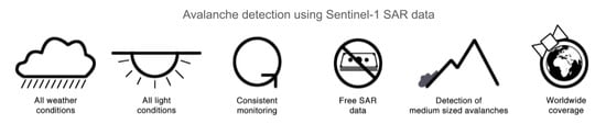
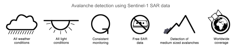
:Knowledge of the spatio-temporal occurrence of avalanche activity is critical for avalanche forecasting. We present a near-real time automatic avalanche monitoring system that outputs detected avalanche polygons within roughly 10 min after Sentinel-1 SAR data are download. Our avalanche detection algorithm has an average probability of detection (POD) of 67.2% with a false alarm rate (FAR) averaging 45.9, with a maximum POD of over 85% and a minimum FAR of 24.9% compared to manual detection of avalanches. The high variability in performance stems from the dynamic nature of snow in the Sentinel-1 data. After tuning parameters of the detection algorithm, we processed five years of Sentinel-1 images acquired over a 150 × 100 km large area in Northern Norway, with the best setup. Compared to a dataset of field-observed avalanches, 77.3% were manually detectable. Using these manual detections as benchmark, the avalanche detection algorithm achieved an accuracy of 79% with high POD in cases of medium to large wet snow avalanches. For the first time, we present a dataset of spatio-temporal avalanche activity over several winters from a large region. Currently, the Norwegian Avalanche Warning Service is using our processing system for pre-operational use in three regions in Norway.
1. Introduction
Snow avalanches (hereafter called avalanches) are rapid mass movements of snow down a hillside or slope occurring in all snow-covered mountain areas worldwide. Improving public avalanche forecasting to reduce fatalities and mitigate damages to infrastructure has a high socio-economic relevance to people living in snow-covered mountain areas. During the last four decades, about 100 people have lost their lives in avalanches each year in the European Alps [1]. Annual financial losses from road closures and infrastructure damages are estimated to be in excess of one billion euros in Europe annually [2].
Conventional public avalanche forecasting (how many avalanches of which size are expected) is carried out by human experts that rely on diverse, incomplete data, with a convenient spatial sample, i.e., what can be easily observed/obtained within the forecast domain. The experts must deal with spatio-temporal scaling issues where data over short time frames from small and not always-representative areas are available. In particular, data on avalanche activity are rarely available at a scale relevant for the entire forecast domain, despite its critical importance in forecasting avalanches [3]. Traditional field-based avalanche monitoring is limited by access to remote areas, observer bias, high avalanche danger and bad visibility. Nevertheless, knowledge about the spatio-temporal occurrence of avalanche activity provides direct evidence of snow instability as well as quantitative data on the consequence factor in the avalanche risk equation (risk = likelihood × consequence).
Remote sensing of avalanches is a young and evolving scientific field. Eckerstorfer et al. [4] provided an overview of avalanche remote sensing using optical, lidar and radar sensors on terrestrial, airborne and space-borne platforms. Which platform-sensor combination should be deployed depends largely on the spatio-temporal scale of the monitoring purpose. The favored choices of technology for avalanche hazard mapping or avalanche activity monitoring at community level for ski resorts or on single slopes, terrestrial sensors. Both optical time-lapse cameras [5] and terrestrial LiDAR scanners [6] have been successfully deployed for continuous slope-scale monitoring. For regional-scale monitoring of avalanche activity, optical- and radar satellite data are the preferred technology. Very high optical satellite data have been used to detect avalanche activity after an extreme avalanche cycle in Switzerland in January 2018. Bühler et al. [7] used Spot 6/7 data to manually delineate over 18,000 avalanches, achieving a high accuracy compared to ground truthing from helicopter reconnaissance. Optical satellite data is, in best case scenarios, highly suitable for avalanche detection and activity monitoring, as all parts of an avalanche, from its starting zone to its depositional area, can be clearly visible. However, cloud cover, shaded areas and polar night darkness are limiting factors for continuous, operational use throughout an entire winter.
Such long-term avalanche monitoring over large regions can only be accomplished using a spaceborne synthetic aperture radar (SAR). Avalanche detection in SAR images has been introduced by Wiesmann et al. [8] using ERS-1 and ERS-2 C-band SAR data. Subsequent studies experimented with X-band TerraSAR-X data [9] and C-band Radarsat-2 Ultrafine mode data [10]. In follow-up studies, C-band SAR data provided by Sentinel-1 were used. [10,11]. Common for these studies, avalanches were detected by expert interpretation of temporal change detection images over time series of up to one winter. Recently, a handful of studies has shown the application of classification and segmentation algorithms for the automatic detection of avalanches in Sentinel-1 data. Eckerstorfer et al. [12] automatically detected avalanche activity in a 150 × 100 km large area during two winters (2016–2018) using multiple Sentinel-1 orbits. Coleou et al. [13] and Karbou et al. [14] used four Sentinel-1 swaths to detect avalanche activity in the French Alps between the end of December 2017 to the end of April 2018. They generally found that their algorithm produced too many false alarms, when putting the detection results into a meteorological context. Recently, the use of neural networks for avalanche segmentation was tested [15,16,17]. Increased activity in the field of SAR-borne avalanche detection likely stems from the free and frequent availability of C-band SAR data provided by the Sentinel-1 constellation almost globally.
The scope of this study is to present a near-real time avalanche activity monitoring system using Sentinel-1 data in Norway in the period of 2014–2019. First, we analyze Sentinel-1 data availability and its spatial coverage in avalanche runout areas. We then present the avalanche detection algorithms logic and performance, validated against expert interpretation (manual detection) and fine-tuned from this comparison. Finally, we introduce an age tracking algorithm and present detected spatio-temporal avalanche activity in the period 2014–2019 in a study area around Tromsø, Norway, which we validate against field observed avalanche activity.
The automatic avalanche detection algorithm used in this study is a further development of the algorithm presented by Vickers et al. [18,19]. Vickers et al. [18] developed an algorithm based on change detection to identify areas where there were potential avalanche debris. These areas were subsequently segmented into two classes using a K-means unsupervised clustering method, the classes representing avalanche and non-avalanche pixels. The algorithm was tested on a small dataset of three S1 image pairs following a wet snow avalanche cycle. The algorithm produced a TSS of 0.7, with PODs ranging between 55% and 68% and corresponding FARs between 27% and 56% compared to manual detections. This algorithm was further developed by Vickers et al. [19] as the varying nature of snow conditions in the S1 images acquired different backscatter thresholds to classify avalanche debris. Although the PODs obtained for the datasets used were not a significant improvement on the earlier version, it was shown that a similar level of performance could be achieved for larger detection areas where meteorological conditions were expected to vary both across the images and between image pairs.
2. Avalanche Activity Monitoring System: Specifications, Data and Workflow
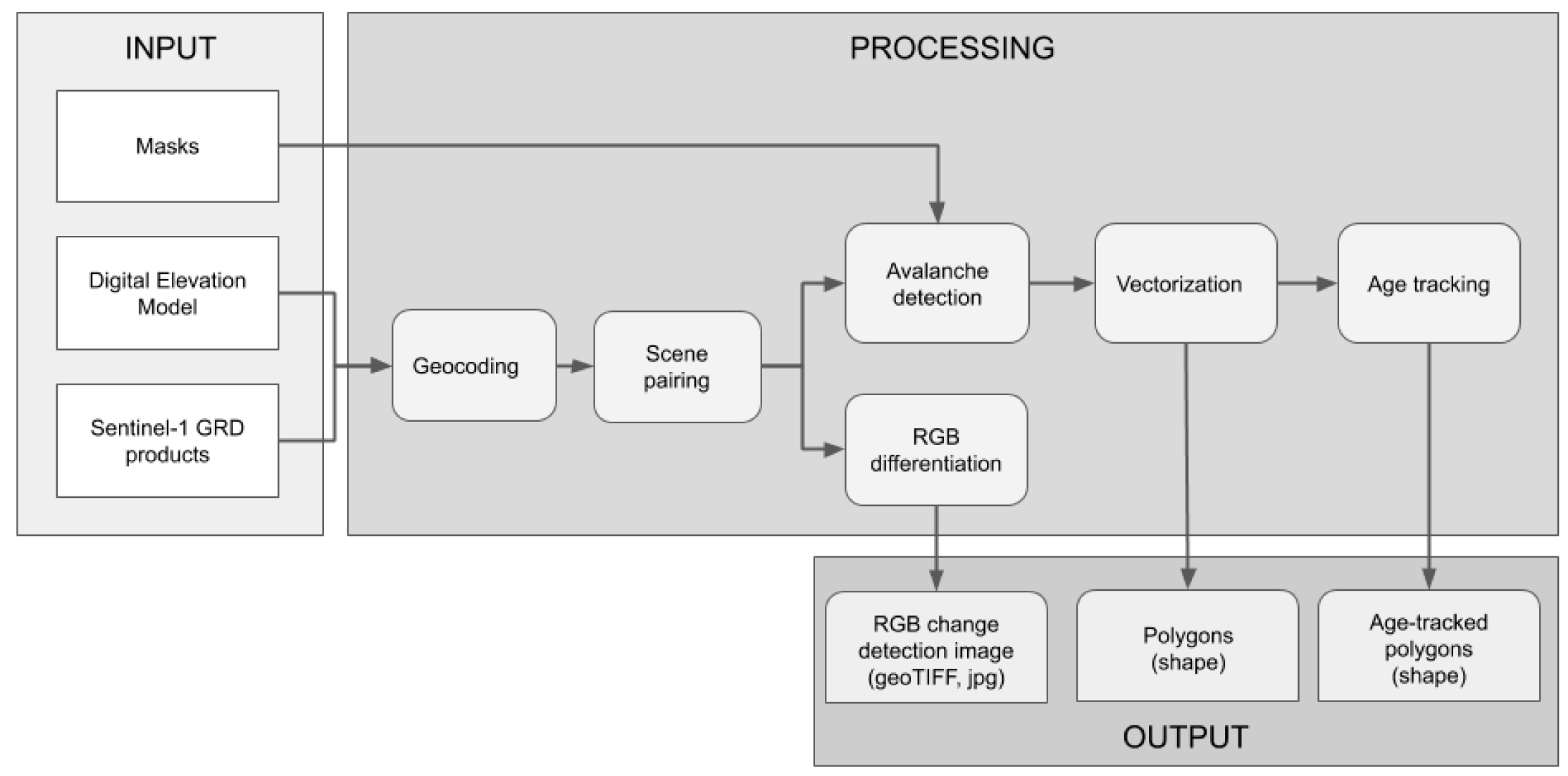
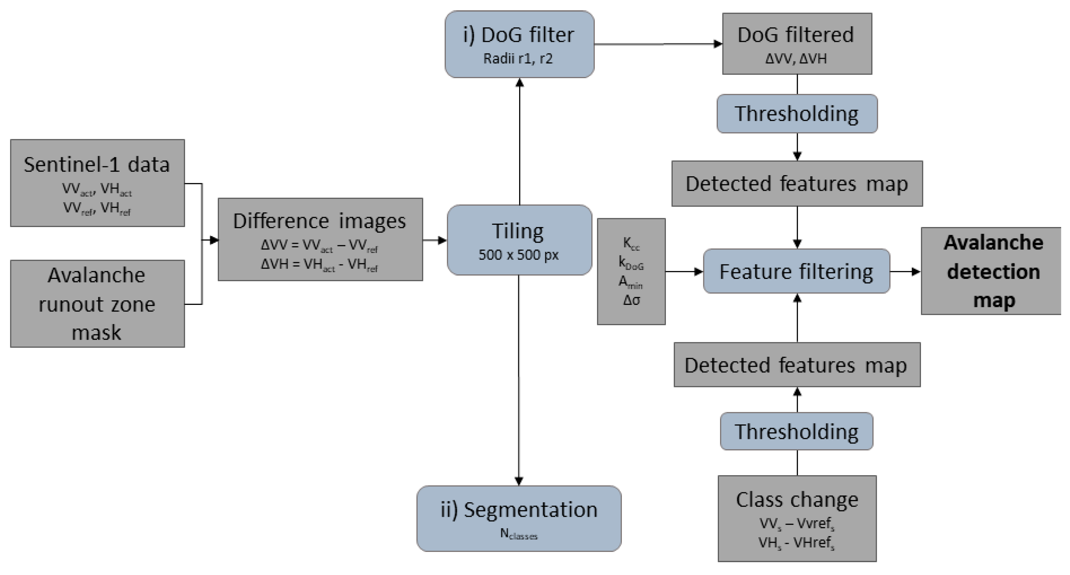
We designed an automatic processing chain that processes three different input data into three different output products (Figure 1). In the following section, we describe each part of the processing chain in detail, starting with the input part that consists of three different data layers that we used:
2.1. Input
2.1.1. Masks
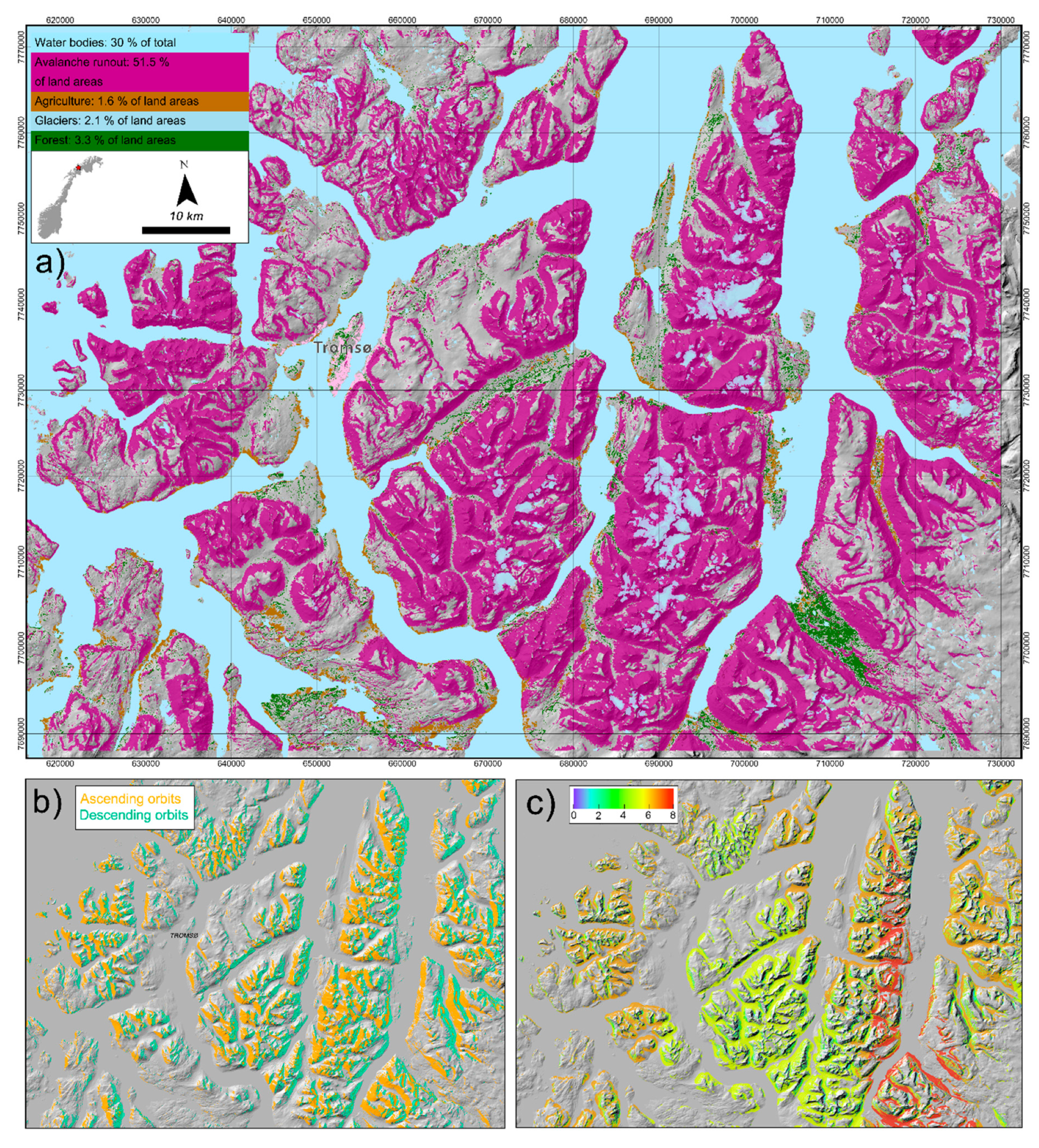
Masks are critical input layers that depict areas in which avalanches can and cannot occur. To reduce computational time, all areas where avalanche occurrence is highly unlikely are masked out. Likewise, to decrease detection uncertainty, a mask is computed that depicts areas where avalanche occurrence is highly likely. If a detected feature occurs in a snow-covered avalanche runout zone, there is a high chance that the feature is an avalanche. Avalanche runout zones are the portion of an avalanche track where avalanches typically stop. A Norway-wide avalanche runout zone mask based on a 10 m DEM, was recently developed [20]. This avalanche runout zone mask was constructed using potential avalanche release areas [21] as a starting point and inferring the avalanche runout by using the TauDEM toolbox available in ArcGIS (http://hydrology.usu.edu/taudem/). This avalanche runout mask eliminates 48.5% of the total study area (Figure 2). Other areas where avalanches are unlikely to occur include water bodies (30% of the total AOI) and forested areas (3.3% of the land areas). Agriculturally used areas (1.6% of the land areas) and glaciated areas (2.1% of the land areas) are masked out due to their sensitivity of surface roughness change (e.g., ploughing in the case of agriculturally used areas), and in the case of glaciers due to their sensitivity to snow cover changes, especially in the early part of the winter.
The study area is centered over the town Tromsø, capital of the county Troms in Northern Norway. The study area is comprised of mountainous topography intersected by fjords and valleys, formed by multiple glaciations. Several small communities, nestled between fjords and steep mountainsides and connected via an extensive road network, lie in avalanche-prone areas.
2.1.2. Digital Elevation Model (DEM)
We used a high-resolution publicly available DEM with a pixel resolution of 10 m and an accuracy of ±1 m. The DEM was constructed using airborne laser scanner data and recently updated in 2018. It is available in UTM 33. The DEM was downloaded from the Norwegian Mapping Authorities’ website (kartkatalog.geonorge.no).
2.1.3. Sentinel-1 GRD Products
The Sentinel-1 constellation consists of two identical satellites (S1A and S1B) that orbit the Earth 180 degree apart. The satellites travel in a sun-synchronous near-polar orbit with the radar instruments illuminating the surface perpendicular to flight direction. Sentinel-1 (S1) data were automatically downloaded from the ESA Open Access Hub (https://scihub.copernicus.eu/) and the Copernicus Collaborative Data Hub (https://colhub.copernicus.eu) using a shell-script that several times a day looked for new S1 data. We defined a roughly 150 × 100 km area centered over Troms County, Norway and all the images that overlap more than 10% with that rectangle were downloaded and processed. S1 GRD (ground range detected) data were downloaded in interferometric wide swath mode (IW mode) with a ground range pixel resolution of 20 m for both VV (vertical transmit and receive) and VH polarization (vertical transmit, horizontal receive). We used GRD products as they are 1/5 the size of SLC products which makes the handling of large data quantities easier. Moreover, GRD products are already radiometrically enhanced, eliminating the need for a single-look complex to multi-look detected processing step on our side.
We downloaded S1 data in the period of 1 December 2014 until 31 May 2019 each year, which is the avalanche forecasting season in Norway. The entire monitoring period had a total of 911 days, of which 590 were covered by S1 data. There is a clear trend towards both increased availability of different swaths as well as the amount of data provided by ESA from 2014 to 2019 (Table 1). This resulted in only 5 days without any S1 data in 2018–2019, while on multiple days, two images were acquirable.
The total extent of the study area encompasses roughly 25.8 million pixel. At maximum, for the ascending geometry, four satellite swaths were available, while six swaths were of descending geometry (Table 1). These swaths exhibited varying spatial coverage of the study area, averaging 58.5% and 75.7% for the ascending orbits and descending orbits, respectively. The lower average spatial coverage of the ascending orbits is mainly due to swath 029 only covering 10.7% of the area. For each swath, radar shadow and layover masks were computed during the geocoding process. As the swaths can vary ±100 m along track, aggregated shadow and layover masks were made from multiple images of each swath. The masked-out areas, due to radar shadow and layover effects, were 11.5% and 14.1% on average for ascending and descending orbits, respectively (Table 1). These masked-out areas lay entirely within the avalanche runout zone. In Figure 2b, we show the areas that are affected by radar shadow and layover in all four ascending and all six descending orbits, respectively.
Considering all the masks applied to the study area and all the satellite swaths available, in 2017–2018, on average, 7.3 S1 images covered the avalanche runout area within a 6-days repeat cycle (Figure 2c). Within a 6-days repeat cycle, all eight available satellite swaths repeated themselves. The avalanche runout area was covered to a varying degree by S1 data with the north-south protruding peninsula in the center-right of the study area, receiving a coverage of eight images, while the central part of the study area received around six images. Nevertheless, slopes of all aspects received only three images per 6-days repeat cycle and 1.3% of the avalanche runout zones were without any coverage.
2.2. Processing
In the following section, we describe the processing steps that lead to three different output data (Figure 1) that we are presenting in this study:
2.2.1. Geocoding
S1 data was geocoded with our inhouse SAR processing software ‘gdar’.‘gdar’ is a generic Python toolkit for processing raster data. The central concept is the ‘gdar’ data raster which combines gridded data (numpy array) with its associated geographical metadata (grid). ‘gdar’ contains readers for a wide range of SAR and optical sensors and a selection of common purpose tools for advanced SAR processing. ‘gdar’ applies proper precision geocoding with an accuracy limited only by orbit and DEM accuracy and precision limited by the quality of the resampling kernel, which is a performance/precision tradeoff. Our geocoding routine is very similar to the Sentinel Application Platform (SNAP) and it has four essential steps:
- Start with the required output map projection (UTM 33N) and a 10 m DEM, projected to the required output grid if necessary.
- Solve range-doppler equations with respect to radar slant range/azimuth coordinates for the grid of 3D positions corresponding to the output grid.
- Convert slant range coordinates to ground range coordinates using the product annotations.
- Resample using calculated precise ground range/azimuth coordinates after converting to subpixel positions in the GRD grid.
- Export sigma nought (radar backscatter) for VV and VH-polarization. Radar backscatter is exported as two separate geotiff-files for the area of interest. In addition, we also export a mask-file defining the layover and shadow regions.
2.2.2. Scene Pairing
Both avalanche detection and RGB differentiation need scene pairing as input. Scene pairing is done with S1 images of similar geometry (ascending or descending) and orbit (e.g., 168). S1 images that are six days apart (twelve days when only Sentinel-1A was in orbit) are paired to produce difference images, showing relative backscatter change.
2.2.3. RGB Differentiation and Avalanche Detection
Avalanche detection in S1 images is based on temporal change detection of backscatter intensity. In the case of an avalanche release, more energy is scattered back to the radar sensor from the avalanche debris relative to that from undisturbed snow [10]. The high backscatter stems to a large degree from the relatively high surface roughness avalanche debris exhibits.
Change detection pairs showing temporal backscatter change are composed both for VV and VH polarization pairs, where. the preceding image is called the reference image (ref) while the current image is called the activity image (act) (Figure 3). RGB differentiation is the process of coloring backscatter change in an RGB image where R(ref), G(act), B(ref). Positive backscatter change in case of avalanches appears in green in these images, while negative backscatter change in case wet snow, for example, appears in purple.
The change detection pairs and the avalanche runout mask function as input to the avalanche detection algorithm (Figure 3). After tiling the input data into 500 × 500-pixel tiles, avalanche detection is carried out in two separate parts: (i) Difference of Gaussians (DoG) filtering and (ii) Segmentation. Both parts are combined after feature filtering to a binary avalanche detection map.
- DoG filtering:A Gaussian filter of radius r1 and a Gaussian filter of radius r2 is applied to the ΔVV and ΔVH images with the Difference of Gaussians image being the result of the difference between the two filtered ΔVV (or ΔVH) images. A threshold is calculated and applied to the DoG filtered difference images using the mean μ and standard deviation of the DoG filtered images. More specifically, we apply two thresholds to the two DoG filtered (ΔVV, ΔVH) images; a lower threshold is defined by μ + 1.5sd and an upper threshold μ + 2.5sd. This yields two interpretations of potential avalanche debris pixels, with the result from the higher threshold representing the greater likelihood of correct detections.
- Segmentation:The four input images are segmented into N classes and used to calculate a class change (i.e., classified activity image–classified reference image) image for the two channels. To distinguish potential avalanche pixels, a threshold is calculated automatically (as with the DoG filtering) from the mean and standard deviation of class change values in the image window. This is done separately for the VV and VH channels. Avalanche debris pixels are those that exceed the threshold in each polarization and a binary map (detected features map) is created, indicating either 0 for “not avalanche” or 1 for “avalanche”.
- Merging of binary maps:The results from the segmentation and DoG filtering are combined to achieve the best possible delineation of the avalanche debris (referred to as “Feature Filtering”) as follows: first, the detected regions from the lower DoG thresholding are taken as a proxy for the avalanche debris. The number of pixels within each region that were also detected from class change thresholding is deduced and converted into a fraction kCC of the total number of pixels within the region. The fraction of pixels within the region that also exceeded the upper DoG threshold, kDoG is also calculated. If both fractions exceed a specified threshold, then the entire detection region is retained; if the criteria are not met, then the detection is nulled out and not considered avalanche debris. In addition, a backscatter contrast Δσ filter is applied to check whether the detected regions are probable candidates for avalanche debris. Here, the backscatter change image is used as a starting point and the difference between the mean backscatter change within (ΔVVIN) and outside (ΔVVOUT) of the detection is calculated (VVContr = ΔVVIN - ΔVVOUT). To calculate the mean backscatter change outside of the detection, a box of a width three times the region width and three times the region height is used to isolate the region of interest. A threshold is applied to determine whether the backscatter contrast is great enough to represent avalanche debris. If the backscatter contrast does not exceed the threshold, then the detected region is again nulled out and does not remain in the final avalanche map. Lastly, a check is performed on the number of pixels in the detected regions, such that if the region area is smaller than minimum Amin of 10 pixels, then the region is not included in the final avalanche map. Vice versa, if the region is larger than maximum Amax of 390 pixels, this corresponds to the largest field validated avalanche detected.
2.2.4. Vectorization
All processing steps from geocoding to avalanche detection are raster-based. The binary avalanche detection map as the final output of the automatic detection algorithm is vectorized and the outline of each detected avalanche is traced to form polygons. In this process, metadata which includes timing of release, location and size of the avalanches are added to the output using topographical information from the DEM.
2.2.5. Age Tracking
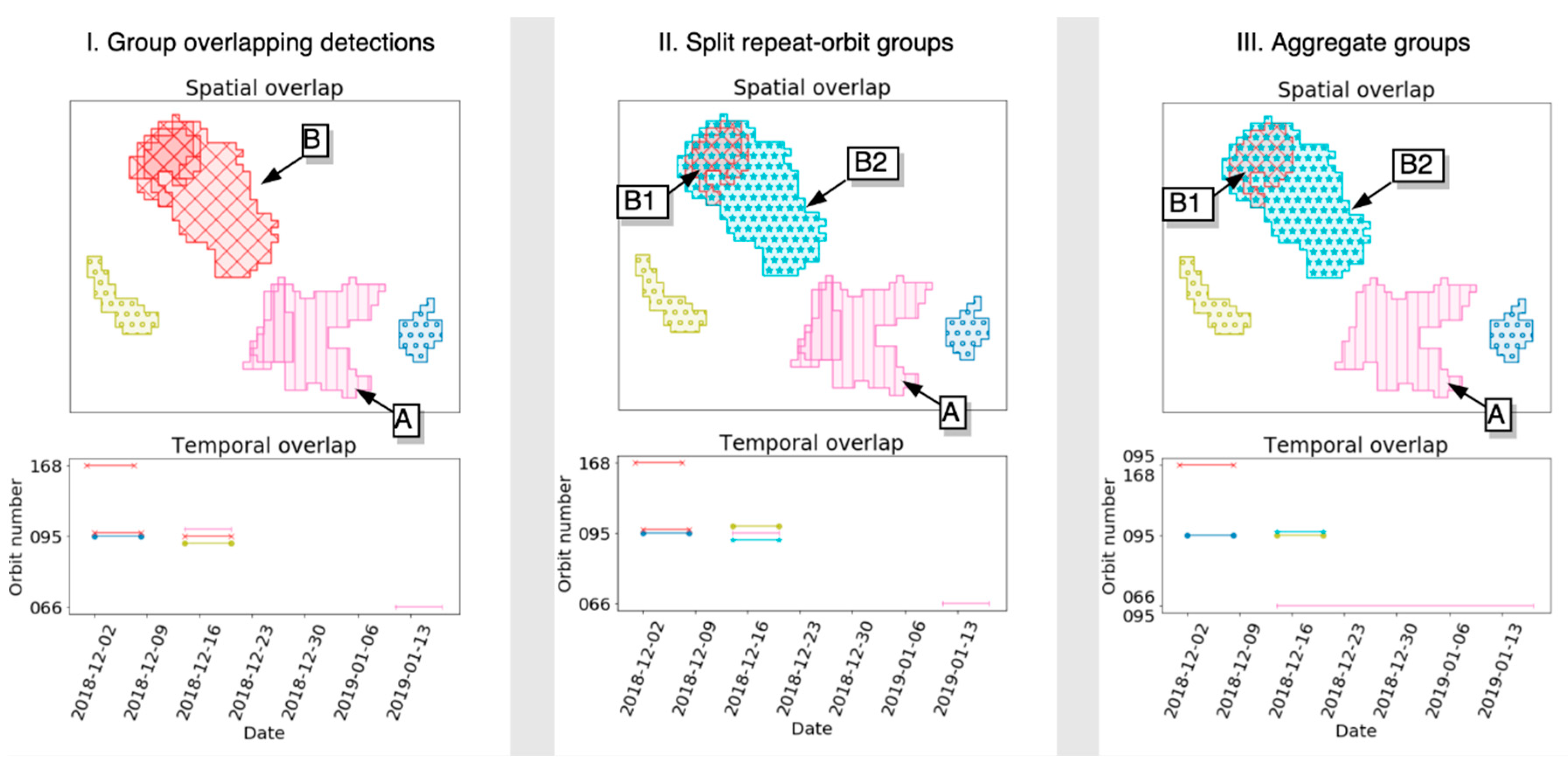
With the availability of multiple overlapping S1 swaths, avalanches are detected multiple times in subsequent S1 images by the detection algorithm. We developed an age tracking algorithm to identify and aggregate multiple detections of the same avalanche. It assumes that if detected, features overlap in time and space and originate from different satellite geometries, they are likely to be the same avalanche. The algorithm can be described by the following three steps (Figure 4):
- Group overlapping detections:In this first step, features detected in multiple images of different orbit overlapping in time (within the 6 days repeat cycle) and space (75% areal overlap) are assumed to be the same avalanche.
- Split repeat orbit groups:If an overlapping group contains multiple detections from the same satellite geometry, the group is split into sub-groups. The split is done in such a way that each resulting sub-group contains at most one detection per satellite geometry, while at the same time, as much overlap as possible between the detections in the resulting sub-groups is preserved. Formally, this is done by representing each detection in the original group as nodes in a graph with the spatial-temporal overlap representing edges between the nodes. If a pair of nodes corresponds to the same satellite orbit, a maximum-flow graph cut is applied between the node pair, resulting in two sub-graphs. The sub-graphs are recursively cut until no pair of nodes corresponding to the same satellite geometry is found.
- Aggregation of groups:Finally, groups that fulfill all requirements from step I are merged into single detections.
The steps are exemplified in Figure 4. In the first step, two groups containing multiple overlapping detections are identified and highlighted by labels A and B. Group A contains two detections corresponding to separate satellite geometries (orbit number 66 and 95). Group B contains one detection from orbit 168 and two from orbit 95. In step two, group B is consequently split into two sub-groups, in the figure labeled B1 and B2. B1 contains two detections (with orbit number 168 and 95) and B2 one detection (with orbit number 95). In step three, the groups (A, B1 and B2) are aggregated into single detections. In a final step, minimum and maximum cutoff sizes for detected features are set to 10 pixels and 390 pixels, respectively, with the maximum cutoff corresponding to the largest detected avalanche in the area of interest.
2.3. Output
The processing chain finally produces three output data, of which two output data are polygons of detected and age tracked avalanches, and one product are RGB change detection images that we use for presentation and expert interpretation (manual detection).
3. Tuning of the Avalanche Activity Algorithm
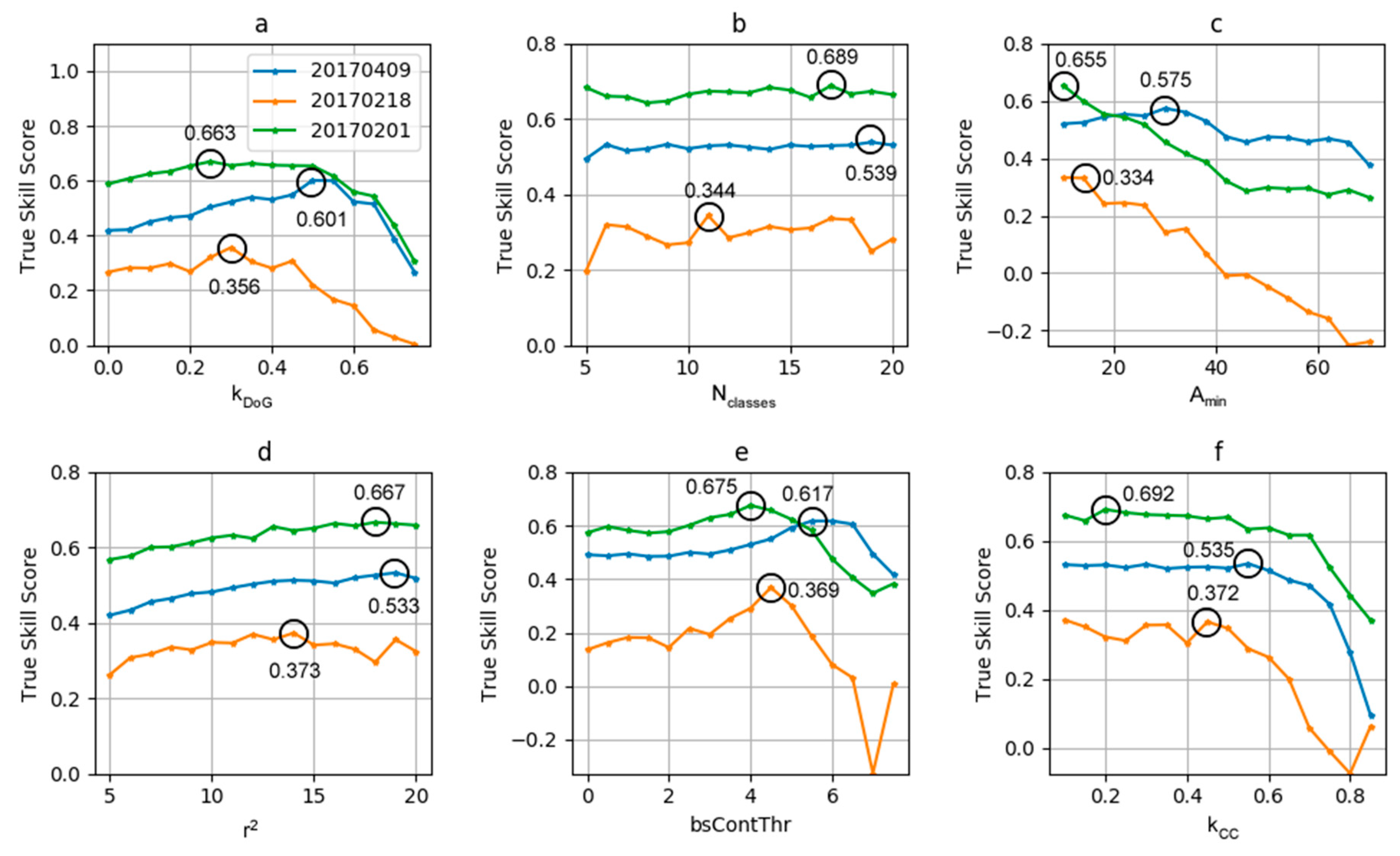
Our avalanche detection algorithm uses six different parameters and thresholds that can be adjusted in order to achieve the best possible detection results. To find an optimal setup, we manually detected avalanches in three different images (20170201, 20170218, and 20170409), each acquired following major avalanche cycles. We manually identified avalanches in RGB change detection images, a technique used by Eckerstorfer and Malnes [10]. We considered manual detection carried out by an expert to be superior to automatic detection and thus used the results as validation and training datasets. We then systematically varied the six parameters outlined in Table 2 in order to obtain different detection outputs that could subsequently be evaluated against the manual detections. Note that only one parameter was varied at a time while keeping the remainders at default values.
The performance was evaluated using probability of detection (POD—ratio of correct automatic detections to total number of manual detections), false alarm rate (FAR—ratio of the number of false automatic detections to the total number) and the true skill score (TSS—difference between POD and FAR). TSS also takes into account the incorrect detections. POD and FAR were based on individual detected features instead of the number of (not) detected pixels.
4. Results
We first present our efforts to tune the automatic avalanche detection algorithm to enhance its performance, then show the results of the avalanche age tracking algorithm that consecutively deleted multiple detections and finally show avalanche activity maps for all the winter seasons between 2014 and 2019 before we validate the output.
4.1. Tuning of Algorithm Parameters to Improve Automatic Detection
Figure 5a shows the TSS for the fraction of pixels in each detection exceeding the upper DoG threshold. There was a general increase in TSS up to an optimal value, which gave the best skill score for all three tested dates. However, the maximum TSS was reached at different thresholds, therefore, we set the optimal value at 0.35 as a compromise between the three dates and to obtain a higher probability of detection, at the risk of a higher false alarm rate.
For the number of classes used in the image segmentation stage (Figure 5b), it is clear that varying this parameter did not have significant effects on the TSS for each dataset and therefore, a value of 12, approximately in the middle of the range investigated was taken to be the updated default value.
The TSS obtained by varying the minimum size of the detected regions that were retained in the final detection map is shown in Figure 5c. Here, it can be seen that the maximum TSS was obtained at minimum avalanche sizes of 10, 14 and 30 pixels on 1 February 2017, 18 February 2017 and 9 April 2017. The new default value was set to 15 since TSS was almost unchanged at this threshold for at least two of the dates while only marginally reduced on 1 February 2017 compared with a minimum size of 10 pixels.
Increasing the radius of the second gaussian filter produced small increases in TSS for all three datasets, as shown in Figure 5d with the range in TSS of around 0.1 over the range of values tested. The maximum TSS was obtained for filter radii of 18, 14 and 19 for 1 February 2017, 18 February 2017 and 9 April 2017, respectively; the “optimal” value was set to 19, since this gave a higher TSS for 18 February 2017 compared with using 18 or 20. TSS for this date was lowest compared with the other two dates, for all values of the filter radius tested.
For the backscatter contrast threshold, which was used to filter out potential false detections, values of 4.0, 4.5 dB and 6.0 dB were found to produce the maximum TSS; however, we see that while 6.0 dB gave the best TSS for the 9 April 2017 dataset, the TSS obtained at this threshold for the two other datasets are 0.2 to 0.3 lower than the maximum TSS achieved for those dates (Figure 5e). Therefore, the default value of 4.0 dB was retained in the optimized version of the algorithm.
Lastly, for the fraction of pixels in the detected region where the class change also exceeded its respective threshold, the results indicate a decreasing TSS for all the dates when the fraction was above 0.5 (original default value) (Figure 5f). Since the TSS is virtually the same at a threshold of 0.1 as at 0.2 on 1 February 2017 and 9 April 2017, a new default value of 0.1 was chosen.
Using the results of tuning the values of the algorithm, we ran the updated algorithm on 14 randomly selected S1 images using the adjusted values of the six parameters investigated. We then compared the automatic detections to manual detections from the same dates. PODs range between 89.5% and 36.4% with an average of 64.7%. FARs range between 81.7% and 25.9% with an average of 45.9%. There is no correlation between high PODs and low FARs. The corresponding TSS ranges between 0.571 and −0.256 with an average of 0.213 (Table 3).
When the false alarm rate is high, the greenness factor (G/RB) tends, to some degree, to be low (r2 = 0.4), suggesting low contrast in the entire paired scene. Finally, the TSS and greenness factor correlate positively (r2 = 0.5), suggesting that a high detection accuracy is achieved in pictures with high contrast.
4.2. Manual Deletion of False Alarms
Based on the large differences in performance depicted in Table 3, we visually the checked days with a high number of automatic avalanche detections. There were 196 days with more than 100 detected avalanches, which we checked against RGB change detection images. Of these 196 days, we deleted 34 days containing a total of 10,361 false alarms. These false alarms were due to wet to dry snow transition between reference and activity image, resulting in a net backscatter increase and thus, difficult detection conditions both manually and automatically. In practice, not much avalanche activity can be expected when the snowpack freezes up. The manual deletion of false alarms due to wet to dry snow transition was only done for the data presentation in Section 4.3 and Section 4.4. Both the accuracy assessment in Table 3 and the comparison to field validations in Section 4.5 were done with the entire automatically detected avalanche activity dataset.
4.3. Spatio-Temporal Avalanche Activity
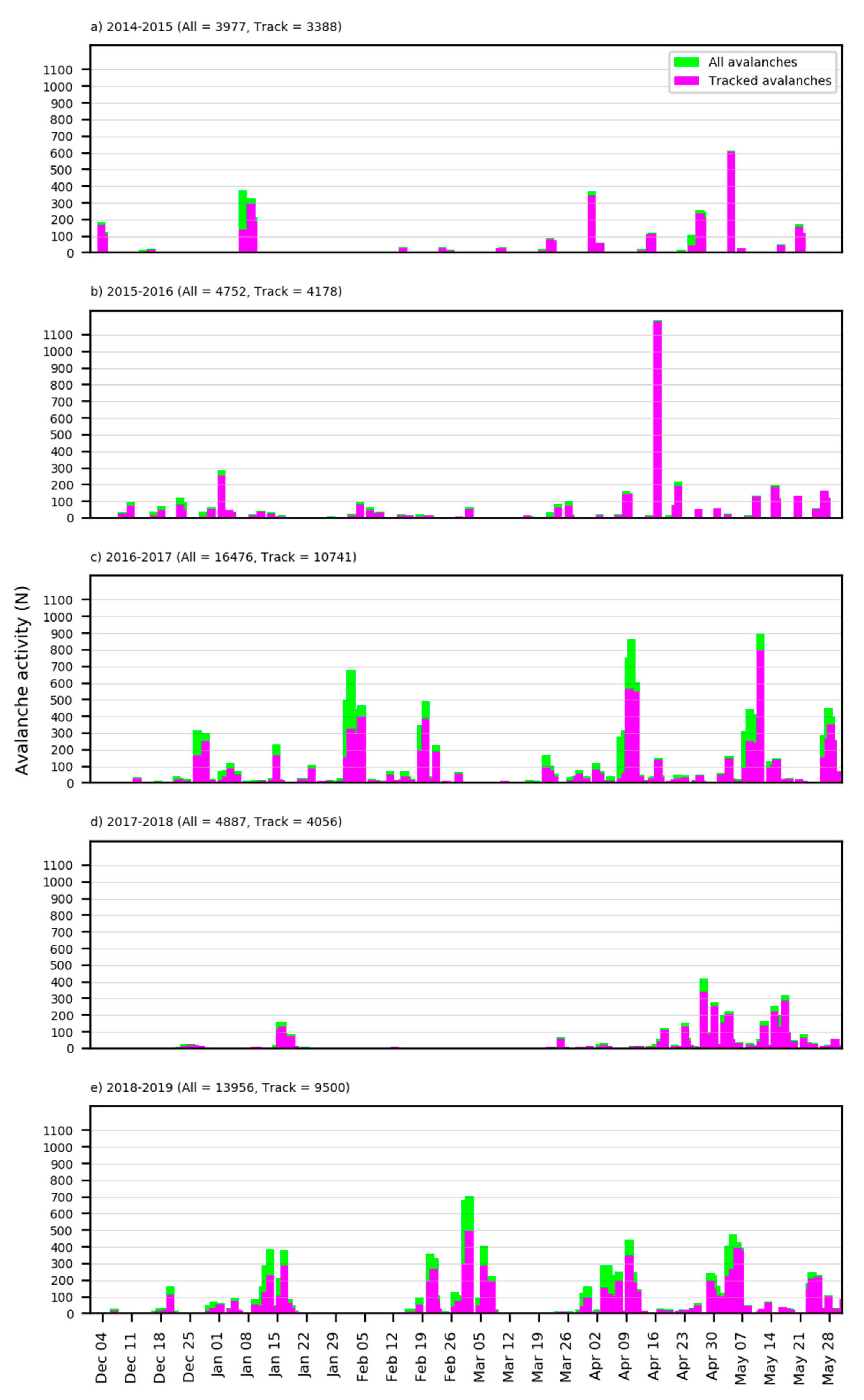
For the first time, we present daily avalanche activity, consistently detected over a five-year period in Troms, Northern Norway (Figure 6). The difference between all and age-tracked avalanche activity varied between winter and was larger when avalanche activity was large. In winter 2016–2017 for example, nearly 35% of all detected avalanches were deleted by the age-tracking algorithm. This makes sense as a high number of daily detections leads also to a high number of multiple detections. There is certainly an observational bias in this dataset that stems from the temporal frequency of S1 data that doubled with the availability of S1B in 2016. As shown in Table 1, both the temporal frequency of S1 data as well as the availability of multiple orbits increased through time. Nevertheless, Figure 6 gives an indication of the overall magnitude of avalanche activity between monitored winters. In particular, winter 2017–2018 was a poor snow winter, resulting in only a third of the avalanche activity detected in 2018–2019. Winter 2017–2018 also had the highest number of high magnitude avalanche days, where over 10 days, more than 450 avalanches were detected.
4.4. Avalanche Activity Map and Time Series
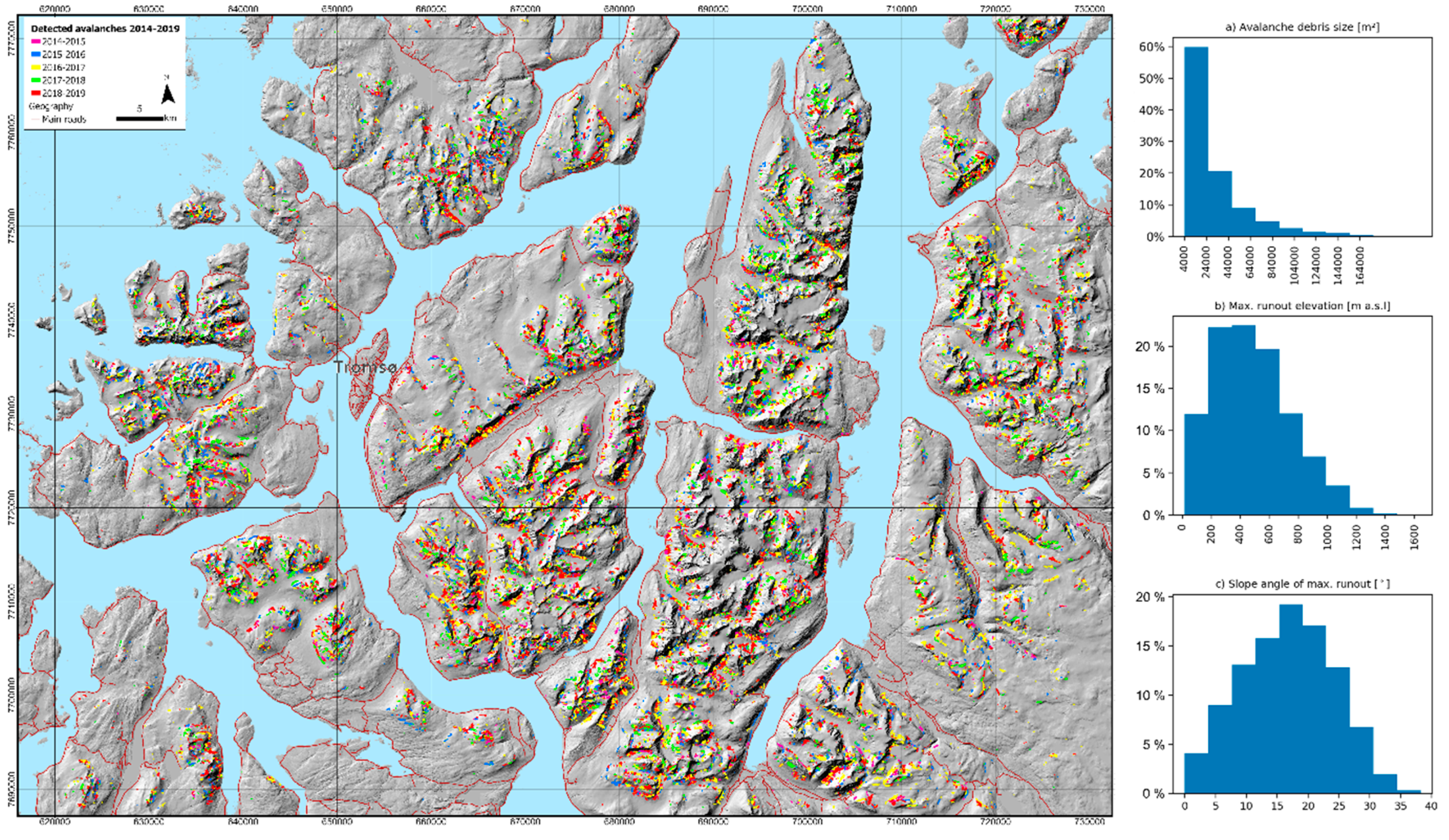
We present both geographical location and outline of every single detected and age tracked avalanche from the 5-year monitoring period in Figure 7. We detected avalanche activity in all high-alpine areas in the area of interest, with most detections located on the prominent north-south trending Lyngen peninsula. There was noteworthy avalanche activity detected along major road infrastructure in the area of interest, with avalanches stopping at a road or even burying it at several places.
The histograms in Figure 7 depict topographical information about all the detected and age-tracked avalanches. Over 50% of the detected avalanches covered an area between 4000 m2 (minimum cutoff) and 24,000 m2, with the size distribution gradually tailing off to a maximum cutoff of almost 222,000 m2. More than 65% of all the avalanches stopped in an elevation zone between 200 and 700 m, however, almost 12% stopped below this zone close to sea level. Finally, the distribution of slope angles at the maximum runout followed a normal distribution.
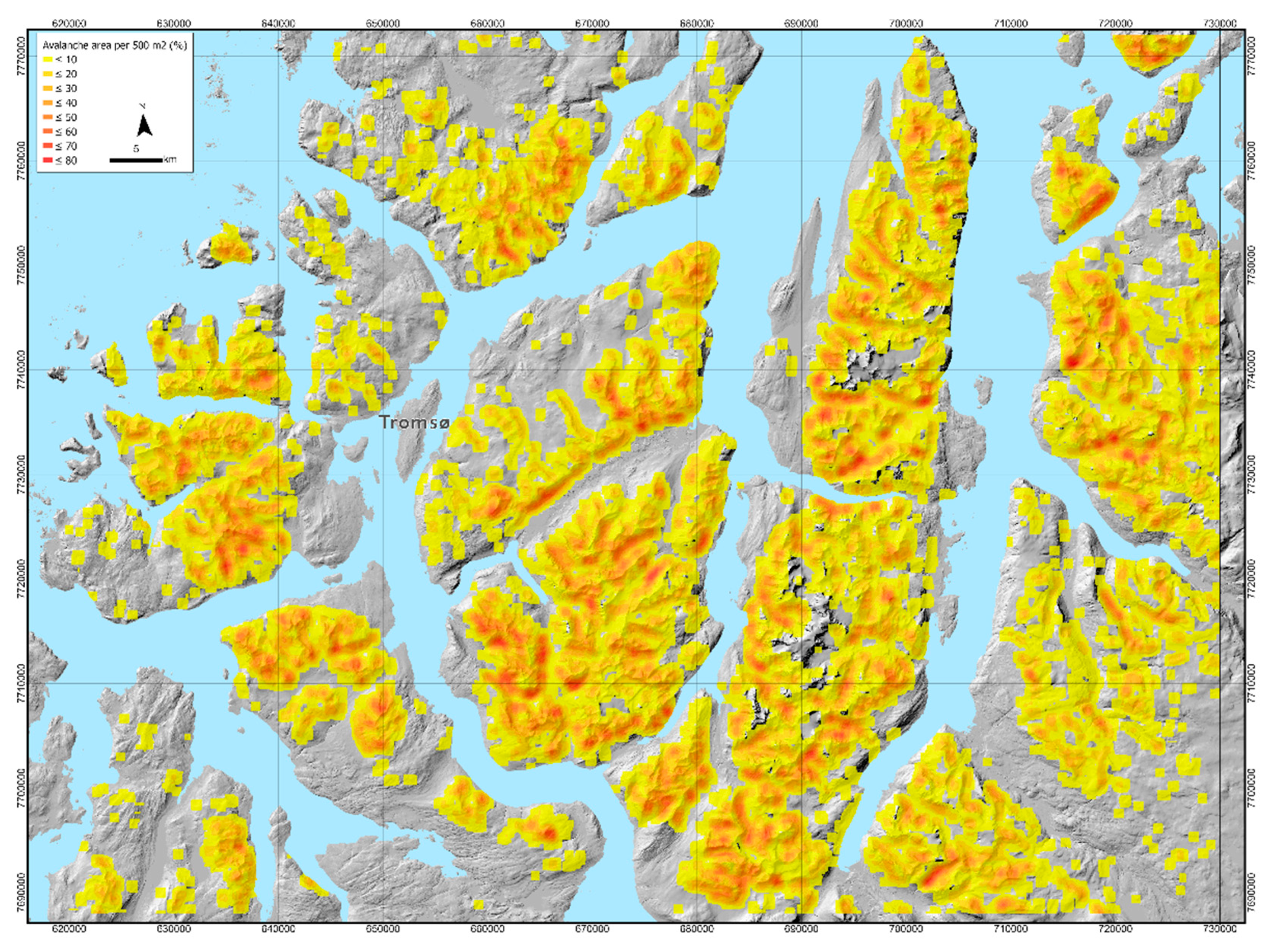
To visualize avalanche-prone areas, we constructed a heat map that shows the percentage of 500 m2 squares covered by avalanches that we detected in the period of 2014–2019 (Figure 8). There are numerous regions where the coverage was as high as 80%, which points both to the occurrence of large avalanches and the frequent reoccurrence of avalanches.
4.5. Field Validation of Manual and Automatic Avalanche Detections
Here, we present a dataset of field-observed avalanches that we used to validate both manual and automatic avalanche detections. Overall, the sample size of field validations is comparably small to the number of detected avalanches. The dataset consists of 243 avalanches that were observed on 26 days, unequally distributed over the period 2014–2019. Comparing field observations with manual detections resulted in a POD of 77.3%, and a POD of 57% when comparing to automatic detections. The probability of manually detecting an avalanche is with 77.3% likely the maximum detection probability using S1 radar satellite data, given the assumption that expert interpretation of SAR change detection images is superior to automatic detection.
We therefore conducted an accuracy assessment comparing the number of manual and automatic detections (Table 4). A true positive rate (sensitivity) of 73% (actual percentage of manual detections that were correctly detected automatically) together with a negative predictive value (proportion of positive and negative results) of 52% was achieved, resulting in an overall accuracy of 79%. This implies that the automatic detection algorithm is quite capable of detecting avalanches that are manually identifiable, however, that there is also quite some room for further improvement.
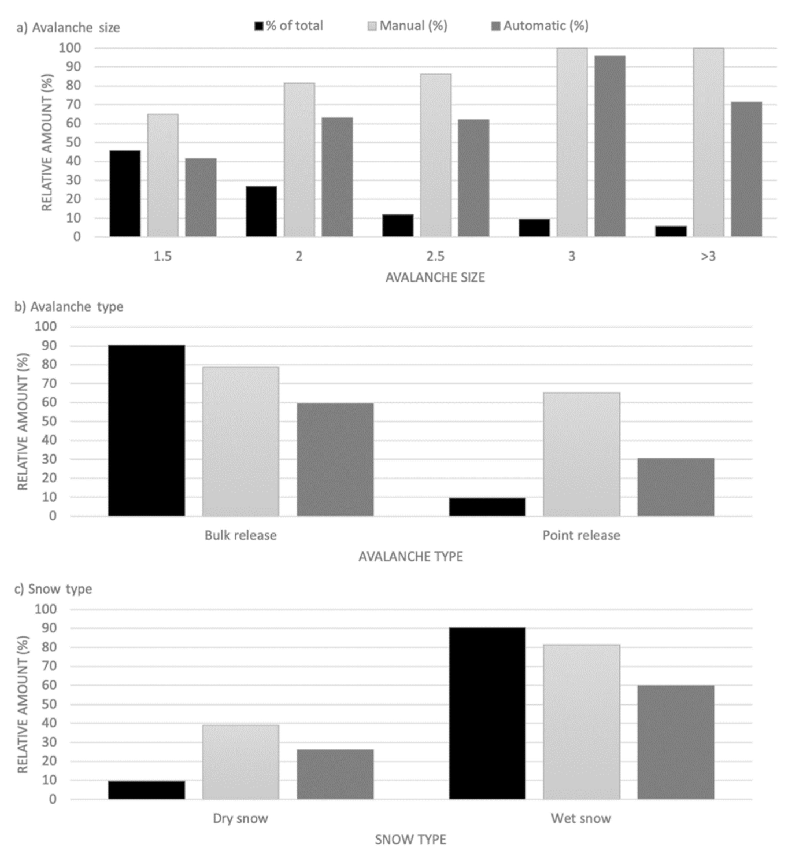
The dataset of field observations, however, allows for a more in-depth analysis of which types and sizes of avalanches were detectable/undetectable both manually and automatically. In our dataset, we have avalanches of different sizes, ranging from small avalanches (size 1.5 and lower) to medium and very large avalanches (size 3 and larger). Over 45% of all avalanches in the dataset were small- to medium-sized avalanches (1–2), where the latter corresponds to typical skier-triggered avalanches (Figure 9a). With increasing avalanche size, the probability of manually detecting them increased from 64.9% (size 1.5) to 100% for size 3 and larger avalanches. There is also an increasing probability of detection for automatic detections with, however, somewhat lower values. Four very large avalanches in the dataset were not detect automatically, resulting in a probability of detection of 71.4%. These slab avalanches were from three different dates, two contained dry and two contained wet snow, and it is unclear to us why we did not detect them.
The vast majority, over 90% of the total, were slab avalanches which release in a bulk (Figure 9b). These slab avalanches dominated the larger avalanche sizes with 95% of the large and 100% of the very large avalanches were slab avalanches. We therefore detected both manually and automatically fewer loose snow avalanches (point release) than slab avalanches (Figure 9b).
Moreover, with 90% of the total, avalanches containing wet snow were prevailing (Figure 9c). With 81.3% manual detections and nearly 59.8% automatic detections, wet snow avalanches were more likely detectable than dry snow avalanches. This distribution is not affected by avalanche size but much more by wet snow avalanches typically exhibiting higher surface roughness than dry snow avalanches, which produces a higher relative backscatter [10].
With surface roughness dominating the backscatter energy from avalanche debris, a qualitative assessment of avalanches that were not detected both manually and automatically hints towards avalanches with low surface roughness being difficult to detect. Another prevailing reason for non-detection are satellite swath timing and geometry. Slopes with field observed avalanche activity were in the radar shadow at first and then not detectable anymore in subsequent S1 images due to various reasons (avalanche debris blown away or snowed in).
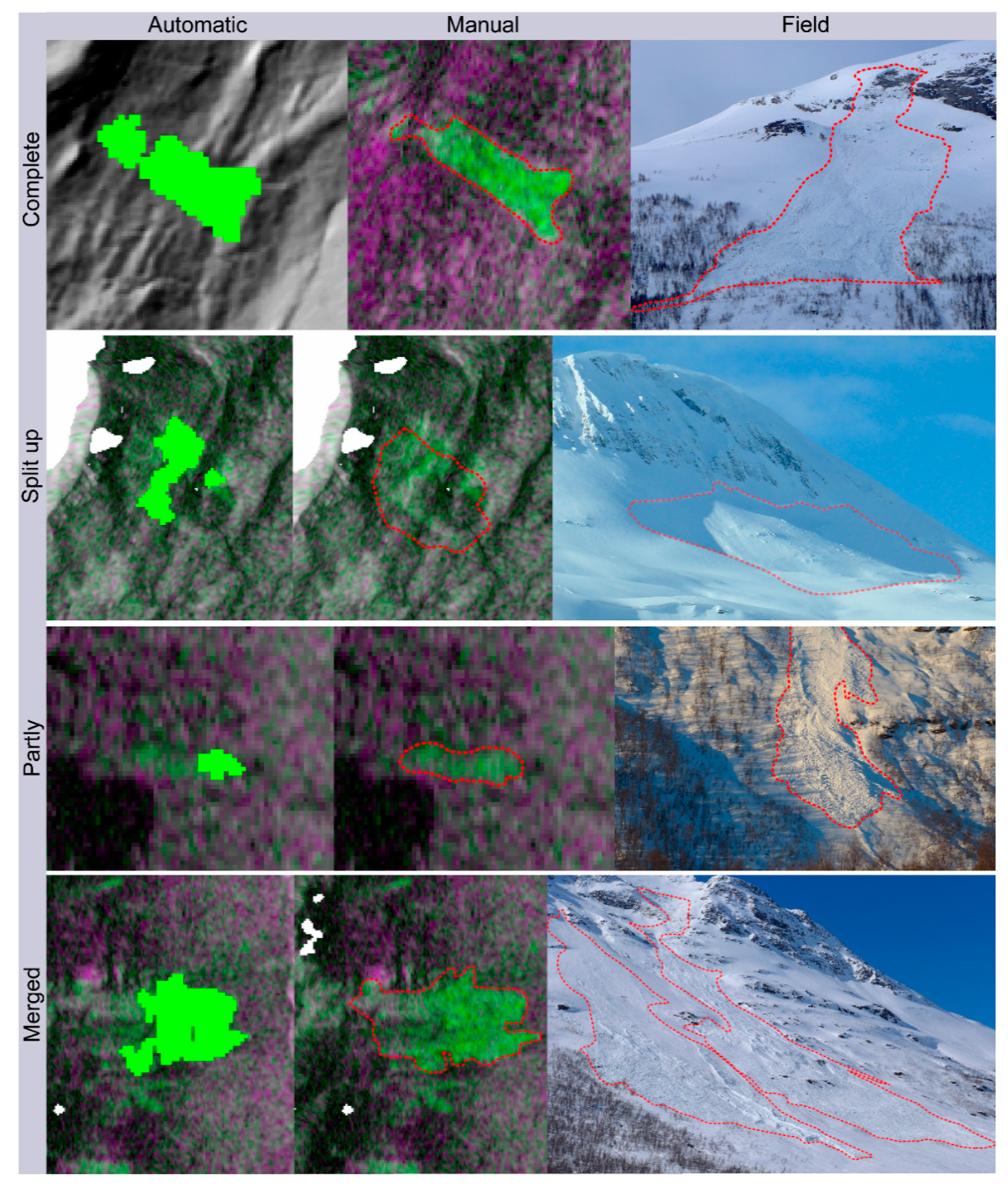
Finally, we qualitatively assessed the accuracy of the automatically detected outlines (N = 138) (Figure 10). By comparing field photographs with the automatically detected outlines, we classified the outlines into completely detected, partly detected (e.g., parts of the debris were not detected), pieces (one avalanche resulted in two detected polygons) or merged (several adjacent avalanches were detected as a single avalanche). Half of the dataset (53.6%) was completely detected, followed by 26.8% of the dataset that were part of a conglomerate of avalanches merged into one and 17.4% were partly detected. There were no statistical relationships between avalanche size and the accuracy of the detected outline. There were, however, twice as many loose snow avalanches in the ‘merged’ category than slab avalanches.
5. Discussion
5.1. Performance of the Automatic Avalanche Detection Algorithm
The version of the algorithm used in this study is a further improvement of the algorithm developed by Vickers et al. [18,19] to address speed issues in order to be able to process much larger volumes of data, which is expected of an operational monitoring service. To achieve this, the K-means clustering technique was replaced with a simplified segmentation module and combined with refined filtering methods to improve the detection results, both in terms of increasing the number of correct detections and reducing false detections. Since both parts of the current algorithm (segmentation + filtering) are dependent on several parameters, we attempted to show that it may be possible to achieve an optimal value for these parameters by using validation data to estimate the performance of the detection results for several datasets and variable ground conditions.
Table 3 shows large differences in POD, FAR and TSS between the validated cases. In best case scenarios, PODs close to 90% were achieved, as well as FARs in the low 20s. On the other hand, we also had test cases with PODs below 35% and FARs above 80%. This large performance variability stems from the algorithm’s dependency of snow conditions in the reference and activity image that build the temporal change detection images. A typical situation favorable for avalanche detection both manually and automatically is when the change detection image exhibits a net decrease in backscatter that creates a large relative backscatter difference between avalanche debris (high backscatter) and surrounding undisturbed snow (low backscatter). This happens when the snow in the reference image is primarily dry and turned wet in the activity image. In these situations, we can suspect that wet snow avalanches occurred if any avalanches were detected. Figure 9 shows that over 80% of all field observed wet snow avalanches were manually detected and 60% automatically. In contrast, wet to dry snow transition results in high false alarms, as explained in Section 4.3.
A possible solution to this dependency on snow conditions might be the use of machine learning for avalanche detection in SAR images. Kummervold et al. [15] used convolutional neural networks on a training dataset of manual detections from varying dates and snow conditions of S1 images to train different neural networks and achieved accuracies consistently over 90%. Waldeland et al. [17] also used neural networks trained on a similar dataset, however, their training dataset contained avalanches that were not manually detected but rather automatically using a set backscatter threshold. They also achieved high accuracies and an average classification error rate of 3.5%. Sinha et al. [16] used a similar approach as the two cited studies above and were able to increase the accuracy of avalanche detection to 77% compared to the 53% accuracy that was achieved by their baseline method [13]. However, common to these studies, binary classification of avalanche/no avalanche was carried out in windows, were the neural network must decide if there is at least one avalanche pixel or not. The problem with this approach is that it is highly dependent on the chosen window size. If the window size is too large, it is more likely to correctly predict the presence of at least one avalanche pixel.
5.2. Comparison to Other Automatic Avalanche Detection Schemes
Similar automatic avalanche detection algorithms to ours do not exist, to our knowledge. Karbou et al. [14]) and Coleou et al. [13] automatically deployed temporal change detection and backscatter thresholding to Sentinel-1 images over the French Alps. Their results show detected and field validated avalanches; however, also a high amount of residual backscatter that was not filtered out. Bühler et al. [22] developed a processing scheme that integrated directional, textural and spectral information from ADS40 airborne digital scanner data to map avalanche deposits. Their method achieved an accuracy of 94% with only small debris in steep terrain not being detected. Lato et al. [23] applied very high-resolution optical images from the QuickBird satellite and the airborne instrument reported by Bühler et al. [22] to apply an object-based image analysis technique to map avalanche debris. In their two case studies, the correct detection rate was above 95%, with a false alarm rate below 5%. Korzeniowska et al. [24] developed the method further, distinguishing between release zone, tracks, and run-out zone. The applicability of these methods, however, was limited by the restrictive availability of the used instrument and the weather and light conditions.
Automatic avalanche detection is also deployed in other non-satellite remote sensing products. Heck et al. [25] used Hidden Markov models to automatically detect avalanches in continuous seismic data from a seismic array deployed above Davos, Switzerland. The Hidden Markov model modelled the seismic time series by a sequence of multivariate Gaussian probability distributions, their characteristics derived from pre-labeled training datasets. After post-processing, PODs ranging between 70% and 90% were achieved. Thüring et al. [26] automatically detected avalanches in infrasound data using supervised machine learning. By using SML, a reduction of false alarms from 65% to 10% was achieved. Finally, real-time automatic avalanche detection systems are available for operational use, using doppler-radar systems for road and infrastructure protection [27]. Avalanches are automatically detected by their motion towards the radar and a trained algorithm filters avalanches from other objects within the line of sight (helicopters for example).
5.3. Limitations and Sources of Error
We identified four major limitations to our avalanche detection scheme:
- Avalanche size: With a pixel spacing of 20 m in our processed S1 images, we are not able to detect small avalanches (unlikely to bury a person, 100 m3) or avalanches that are thinner than then sub-pixel spacing. Since we are aware of this, we have a cut-off minimum avalanche size of 10 pixels. By doing so, we can reduce the false alarm rate significantly. The detection of smaller avalanches will only be possible with higher spatial resolution SAR sensors. Eckerstorfer and Malnes [10] showed that more and smaller avalanches were detectable in very high resolution Radarsat-2 images compared to Sentinel-1 images. Future sensor constellations may provide higher spatial resolution while maintaining or increasing the temporal/spatial coverage of Sentinel-1, and thus opening for the possibility of detecting small avalanches.
- S1 data availability: For complete, near-real time avalanche detection in large regions throughout an entire winter, reliable S1 data availability is of critical importance. The S1 acquisition plan is not predictable and prone to changes. The disappearance of satellite orbits can then be especially troubling in areas at lower latitude that are covered by less orbits to begin with.
- Wet to dry snow transition: We are certainly over-detecting avalanches over the course of a winter with respect to the avalanche sizes we are capable of detecting. The single major contributor to a high false alarm rate is the change in snow conditions from wet to dry in the images that compose the change detection image we use for detection. We thus deleted the days with high false alarms resulting from wet to dry snow transition, assuming that widespread avalanche activity is unlikely when snow dries up, as the snowpack typically stabilizes and consolidates. However, this manual intervention is not ideal, especially in a near-real time monitoring scenario. A possible solution would be to automatically flag these instances of wet to dry snow transition by simply detecting wet snow in the SAR images, following a backscatter intensity thresholding method by Nagler and Rott [28].
- Radar shadow and layover areas: With the SAR instruments on board the S1 satellites being sideways looking radars, radar shadow and layover affected areas are introduced to the images. In these areas, avalanche detection is not possible. The effect of these masked out areas is in our study area negligible as most affected areas are nevertheless masked out by the avalanche runout zone mask. Nevertheless, in areas with very steep topography, radar shadow and layover affected areas could to a large degree reduce the detectable area.
- Sources of false alarms: It is not possible to determine from C-band SAR data if there is dry snow on the ground or no snow. This can lead to false alarms from changing agricultural areas, man-made infrastructure, glaciers, debris flow channels and rock fall scars. By consistently monitoring our area of interest over the past five years, we were able to identify problematic areas that led to many false alarm rates and masked them out.
5.4. Global Application of Near-Real Time Avalanche Monitoring Using S1
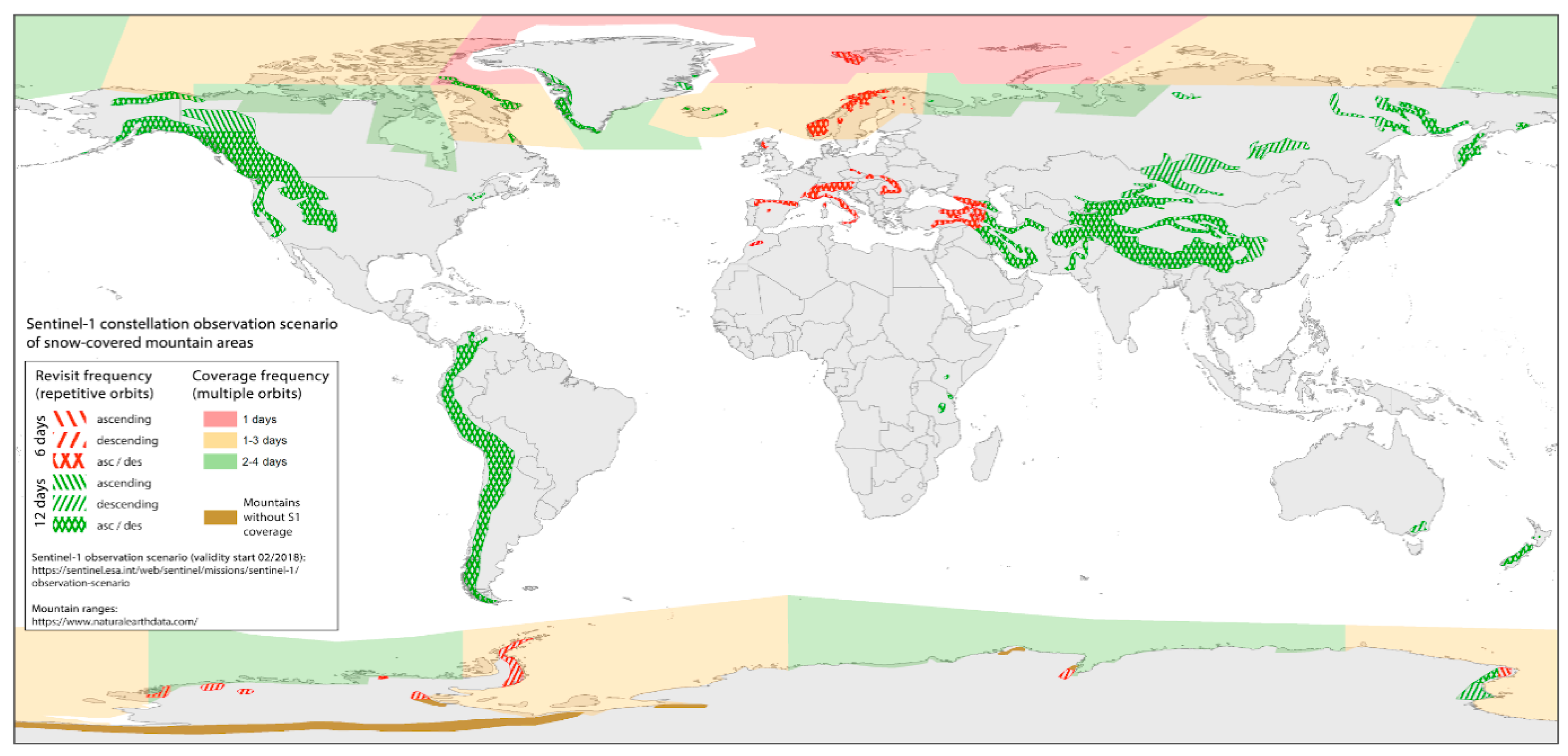
All processing steps and input data of our avalanche detection system are generic, thus the processing chain can be applied to any snow-covered mountain area worldwide, given that S1 data are available. We therefore used the K3 dataset from the GOE Global Network for Observation and Information in Mountain Environments to define global mountain regions. In this K3 dataset, we selected ‘High Mountains’ and ‘Scattered High Mountains’ and superimposed the global Sentinel-1 constellation observation scenario map. Figure 11 shows revisit frequencies of repetitive orbits (satellite swaths) for mountain regions where avalanches can occur. Except for Antarctica, where S1 coverage is in general thin, all snow-covered mountain regions worldwide are covered by at least one satellite swath with a revisit frequency of 12 days. Europe is covered both with ascending and descending orbits with a revisit frequency of 6 days. High-latitude areas receive up to daily revisit frequencies due to multiple orbits.
In theory, the current S1 constellation observation scenario allows for avalanche detection globally, except for the Transantarctic Mountain Range. In practice, the spatio-temporal coverage of S1 data in different mountain ranges sets limitations to the idea of consistent near-real time monitoring of avalanche activity. For near-real time avalanche activity monitoring throughout a winter, the following pre-requisites are needed:
- The forecasting region lies in Europe, ensuring 6-days repeat cycles and coverage at least every second day. Ideally, there is an even distribution of available ascending and descending orbits to ensure that all slope aspects are monitored equally.
- The forecasting region has a geometry that ensures complete coverage by only a few S1 orbits. Complete spatial coverage by S1 data is not only dependent on the regions’ spatial extent, but more so on its geometry relative to the footprint of S1 images. Norway is ideal as it stretches North-South and can thus be covered by only a few orbits with high frequency. If a region stretches rather East-West, more S1 orbits are required to cover the region in its entirety.
- Enough field observations should be available to validate the avalanche detections.
6. Conclusions
The ability to monitor avalanche activity consistently throughout an entire winter in a given region is of high interest for avalanche forecasting and hazard mapping. This goal became more attainable with the use of Sentinel-1 radar satellite data for avalanche detection. In this study, we introduced an automatic processing chain that transforms Sentinel-1 GDR products into detected avalanche polygons within roughly 10 min. The processing system was designed to detect avalanches reliably and constantly over an entire winter in near-real time during all weather and light conditions. The generic nature of input data makes worldwide application of the processing system possible, given the availability of Sentinel-1 data.
We tuned six parameters of the avalanche detection algorithm and tested the best setup on a dataset of 14 Sentinel-1 images. Compared to manual detections, the algorithm produced an average true skill score of 0.213, with a high variation in detection probability and false alarm rate due to the dynamic nature of snow in the Sentinel-1 images. We then ran the processing chain that also includes an age-tracking algorithm which eliminates multiple detections of the same avalanches, on five winters (2014–2019) of Sentinel-1 data in an area surrounding the town of Tromsø in Northern Norway. This dataset of avalanche detections is the first of its kind worldwide, providing spatio-temporal information on avalanche activity in a large region (150 × 100 km). Compared to a dataset of field-observed avalanches, 57% were automatically detected. However, using manual interpretation as benchmark, an accuracy of 79% was achieved.
The presented automatic avalanche processing system is currently pre-operationally used in three regions in Norway by the Norwegian Avalanche Warning Service. They use the daily updated avalanche activity map to gain a spatially more representative view of avalanche activity within each region. This helps them to verify their avalanche risk assessment that was given on the day before and reduces uncertainty in either increasing or decreasing the given avalanche danger level. Recent publications have indicated that deep learning methods can yield improved detection results. Further research is required to test neural networks on entire Sentinel-1 images, detecting avalanches on a pixel scale. Until then, our method presented in this study acts as the benchmark in automatic avalanche detection using Sentinel-1 radar satellite data.
Author Contributions
M.E. carried out the funding acquisition and project administration, conceptualized this study, curated the data and wrote the original draft. H.V., E.M. and J.G. developed the software, wrote, reviewed and edited the manuscript.
Funding
This research was funded by the Norwegian Space Centre, the Norwegian Water and Energy Directorate and the Norwegian Public Road Administration, grant number NIT.18.17.5.
Acknowledgments
We acknowledge the useful comments by two anonymous reviewers that helped improve the readability of this study.
Conflicts of Interest
The authors declare no conflict of interest.
References
- Techel, F.; Stucki, T.; Margreth, S.; Marty, C.; Winkler, K. Schnee und Lawinen in den Schweizer Alpen. Hydrologisches Jahr 2013/2014. 2015. Available online: https://www.slf.ch/de/publikationen/schnee-und-lawinen-in-den-schweizer-alpen-hydrologisches-jahr-201314.html (accessed on 28 October 2019).
- Rudolf-Miklau, F.; Sauermoser, S. The Technical Avalanche Protection Handbook; Mears, A.I., Ed.; Wiley Ernst & Sohn: Berlin, Germany, 2015. [Google Scholar]
- McClung, D.M. The Elements of Applied Avalanche Forecasting, Part II: The Physical Issues and the Rules of Applied Avalanche Forecasting. Nat. Hazards 2002, 26, 131–146. [Google Scholar] [CrossRef]
- Eckerstorfer, M.; Bühler, Y.; Frauenfelder, R.; Malnes, E. Remote sensing of snow avalanches: Recent advances, potential, and limitations. Cold Reg. Sci. Technol. 2016, 121, 126–140. [Google Scholar] [CrossRef]
- Vogel, S.; Eckerstorfer, M.; Christiansen, H.H. Cornice dynamics and meteorological control at Gruvefjellet, Central Svalbard. Cryosphere 2012, 6, 157–171. [Google Scholar] [CrossRef]
- Hancock, H.; Prokop, A.; Eckerstorfer, M.; Hendrikx, J. Combining high spatial resolution snow mapping and meteorological analyses to improve forecasting of destructive avalanches in Longyearbyen, Svalbard. Cold Reg. Sci. Technol. 2018, 154, 120–132. [Google Scholar] [CrossRef]
- Bühler, Y.; Hafner, E.D.; Zweifel, B.; Zesiger, M.; Heisig, H. Where are the avalanches? Rapid mapping of a large snow avalanche period with optical satellites. Cryosphere Discuss 2019. in review. [Google Scholar] [CrossRef]
- Wiesmann, A.; Wegmueller, U.; Honikel, M.; Strozzi, T.; Werner, C.L. Potential and methodology of satellite based SAR for hazard mapping. In Proceedings of the IEEE 2001 International Geoscience and Remote Sensing Symposium, Sydney, Australia, 9–13 July 2001. [Google Scholar]
- Bühler, Y.; Bieler, C.; Pielmeier, C.; Wiesmann, A.; Caduff, R.; Frauenfelder, R.; Jaedicke, C.; Bippus, G. All-weather avalanche activity monitoring from space? In Proceedings of the International Snow Science Workshop 2014, Banff, Canada, 29 September–3 October 2014; pp. 795–802. [Google Scholar]
- Eckerstorfer, M.; Malnes, E. Manual detection of snow avalanche debris using high-resolution Radarsat-2 SAR images. Cold Reg. Sci. Technol. 2015, 120, 205–218. [Google Scholar] [CrossRef]
- Malnes, E.; Eckerstorfer, M.; Vickers, H. First Sentinel-1 detections of avalanche debris. Cryosphere Discuss. 2015, 9, 1943–1963. [Google Scholar] [CrossRef]
- Eckerstorfer, M.; Malnes, E.; Vickers, H.; Müller, K.; Engeset, R.; Humstad, T. Operational avalanche activity monitoring using radar satellites: From Norway to worldwide assistance in avalanche forecasting. In Proceedings of the International Snow Science Workshop Proceedings 2018, Innsbruck, Austria, 7–12 October 2018; pp. 333–337. [Google Scholar]
- Coleou, C.; Karbou, F.; Deschartes, M.; Martin, R.; Dufour, A.; Eckert, N. The use of SAR satellite observations to evaluate avalanche activities in the French Alps during remarkable episodes of the 2017-2018 season. In Proceedings of the International Snow Science Workshop 2018, Innsbruck, Austria, 7–12 October 2018; pp. 392–395. [Google Scholar]
- Karbou, F.; Coleou, C.; Lefort, M.; Deschatres, M.; Eckert, N.; Martin, R.; Charvet, G.; Dufour, A. Monitoring avalanche debris in the French mountains using SAR observations from Sentinel-1 satellites. In Proceedings of the International Snow Science Workshop 2018, Innsbruck, Austria, 7–12 October 2018; pp. 344–347. [Google Scholar]
- Kummervold, P.E.; Malnes, E.; Eckerstorfer, M.; Arntzen, I.M.; Bianchi, F. Avalanche detection in Sentinel-1 radar images using convolutional neural networks. In Proceedings of the International Snow Science Workshop 2018, Innsbruck, Austria, 7–12 October 2018; pp. 377–381. [Google Scholar]
- Sinha, S.; Giffard-Roisin, S.; Karbou, F.; Deschatres, M.; Karas, A.; Eckert, N.; Coléou, C.; Monteleoni, C. Can Avalanche Deposits be Effectively Detected by Deep Learning on Sentinel-1 Satellite SAR Images? In Proceedings of the Climate Informatics, Paris, France, 2–4 October 2019. [Google Scholar]
- Waldeland, A.U.; Reksten, J.H.; Salberg, A.-B. Avalanche Detection in Sar Images Using Deep Learning. In Proceedings of the IGARSS 2018 IEEE International Geoscience and Remote Sensing Symposium, Valencia, Spain, 22–27 July 2018; pp. 2386–2389. [Google Scholar]
- Vickers, H.; Eckerstorfer, M.; Malnes, E.; Larsen, Y.; Hindberg, H. A method for automated snow avalanche debris detection through use of synthetic aperture radar (SAR) imaging. Earth Space Sci. 2016, 3, 446–462. [Google Scholar] [CrossRef]
- Vickers, H.; Eckerstorfer, M.; Malnes, E.; Doulgeris, A.; Sharma, P.; Bianchi, F.M. Synthetic Aperture Radar (SAR) Monitoring of Avalanche Activity: An Automated Detection Scheme. In Computer Vision—ECCV 2012; Springer Science and Business Media LLC: Berlin, Germany, 2017; Volume 10270, pp. 136–146. [Google Scholar]
- Larsen, H.T.; Hendrikx, J.; Slåtten, M.S.; Engeset, R.V. GIS based ATES mapping in Norway, a tool for expert guided mapping. In Proceedings of the International Snow Science Workshop 2018, Innsbruck, Austria, 7–12 October 2018; pp. 1604–1608. [Google Scholar]
- Veitinger, J.; Sovilla, B. Linking snow depth to avalanche release area size: measurements from the Vallée de la Sionne field site. Nat. Hazards Earth Syst. Sci. 2016, 16, 1953–1965. [Google Scholar] [CrossRef]
- Lato, M.J.; Frauenfelder, R.; Bühler, Y. Automated detection of snow avalanche deposits: segmentation and classification of optical remote sensing imagery. Nat. Hazards Earth Syst. Sci. 2012, 12, 2893–2906. [Google Scholar] [CrossRef]
- Bühler, Y.; Hüni, A.; Christen, M.; Meister, R.; Kellenberger, T. Automated detection and mapping of avalanche deposits using airborne optical remote sensing data. Cold Reg. Sci. Technol. 2009, 57, 99–106. [Google Scholar] [CrossRef]
- Korzeniowska, K.; Bühler, Y.; Marty, M.; Korup, O. Regional snow-avalanche detection using object-based image analysis of near-infrared aerial imagery. Nat. Hazards Earth Syst. Sci. 2017, 17, 1823–1836. [Google Scholar] [CrossRef]
- Heck, M.; Hammer, C.; van Herwijnen, A.; Schweizer, J.; Fäh, D. Automatic detection of snow avalanches in continuous seismic data using hidden Markov models. Nat. Hazards Earth Syst. Sci. 2018, 18, 383–396. [Google Scholar] [CrossRef]
- Thüring, T.; Schoch, M.; van Herwijnen, A.; Schweizer, J. Robust snow avalanche detection using supervised machine learning with infrasonic sensor arrays. Cold Reg. Sci. Technol. 2015, 111, 60–66. [Google Scholar] [CrossRef]
- Meier, L.; Jacquemart, M.; Blattmann, B.; Arnold, B. Real-Time Avalanche Detection with Long-Range, Wide-Angle Radars for Road Safety in Zermatt, Switzerland. In Proceedings of the International Snow Science Workshop 2016, Breckenridge, CO, USA, 3–7 October 2016; pp. 304–308. [Google Scholar]
- Nagler, T.; Rott, H. Retrieval of wet snow by means of multitemporal SAR data. IEEE Trans. Geosci. Remote. Sens. 2000, 38, 754–765. [Google Scholar] [CrossRef]
Figure 1.
Workflow of the processing chain for automatic avalanche detection using Sentinel-1 data.

Figure 2.
(a) Avalanche runout mask (purple), water bodies, agricultural and forested areas superimposed onto a hill shade map of the area of interest. (b) Masks due to layover and radar shadow in ascending and descending orbits, (c) average amount of Sentinel-1 coverage per 6 days repeat cycle for avalanche runout zones in the study area in 2017–2018. Areas without Sentinel-1 coverage are shown as shaded areas.

Figure 3.
Logic and steps of automatic avalanche detection.

Figure 4.
Flow chart describing the avalanche age tracking algorithm.

Figure 5.
Variation of True Skill Score for each parameter that was tested (compare to Table 2), and for each of the three datasets. (a) Fraction of pixels in region > upper DoG threshold (kDoG), (b) Number of classes for image segmentation (Nclasses), (c) Minimum avalanche size (Amin), (d) Filter radius of second Difference of Gaussians filter (r2), (e) Backscatter contrast (false detection filter) (bsContThr), (f) Fraction of pixels in region > class change threshold (kCC).

Figure 6.
Time series of daily avalanche detections with all detections in green and age tracked detections in magenta for all five winters in the period of 2014–2019. The numbers in the upper left corner indicate the total number of all detections and age tracked detections.
Figure 6.
Time series of daily avalanche detections with all detections in green and age tracked detections in magenta for all five winters in the period of 2014–2019. The numbers in the upper left corner indicate the total number of all detections and age tracked detections.

Figure 7.
Avalanche activity map with the location of detected avalanches superimposed onto a hillshade map. The colors represent the detected avalanche activity for each of the five winters. The three histograms on the right side depict the distributions of (a) avalanche debris size, (b) maximum runout elevation, and (c) slope angle of maximum runout for the entire 2014–2019 age-tracked dataset (N = 31863).

Figure 8.
Heat map showing the percentage of 500 m2 squares covered by detected avalanches (2014–2019).
Figure 8.
Heat map showing the percentage of 500 m2 squares covered by detected avalanches (2014–2019).

Figure 9.
Manual and automatically detected avalanches classified by their size, avalanche type and snow type.
Figure 9.
Manual and automatically detected avalanches classified by their size, avalanche type and snow type.

Figure 10.
Outline accuracy of automatic detections compared to manual interpretation of RGB change detection images and field photographs.
Figure 10.
Outline accuracy of automatic detections compared to manual interpretation of RGB change detection images and field photographs.

Figure 11.
Sentinel-1 constellation observation scenario of snow-covered mountain regions with validity starting February 2018. This map is modified from a map published at https://sentinel.esa.int/web/sentinel/missions/sentinel-1/observation-scenario. Snow-covered mountain regions were inferred from the Global Mountain Explorer raster dataset of global mountain regions.


Table 1.
Temporal coverage of S1 satellite swaths for each of the monitored avalanche forecasting seasons.
Table 1.
Temporal coverage of S1 satellite swaths for each of the monitored avalanche forecasting seasons.
| Avalanche Forecasting Seasons (1 December–31 May) | Spatial Coverage (%) | Radar Shadow & Layover Areas (%) | |||||
|---|---|---|---|---|---|---|---|
| Orbits | 2014–2015 (N) | 2015–2016 (N) | 2016–2017 (N) | 2017–2018 (N) | 2018–2019 (N) | ||
| 029-ASC | - | - | 28 | 31 | 28 | 10.7 | 0.5 |
| 087-ASC | - | - | 13 | 29 | 29 | 42.2 | 13.4 |
| 131-ASC | 14 | 14 | 26 | 29 | 30 | 100 | 11.2 |
| 160-ASC | 12 | 15 | 27 | 26 | 28 | 81 | 20.9 |
| Ascending | 58.5 | 11.5 | |||||
| 022-DES | - | - | 13 | 31 | 30 | 100 | 5.5 |
| 058-DES | - | - | 28 | 28 | 30 | 94.1 | 16.6 |
| 066-DES | - | 15 | 27 | 29 | 29 | 100 | 24.5 |
| 095-DES | 4 | 15 | 28 | 31 | 31 | 28.5 | 14.9 |
| 139-DES | - | 11 | 28 | 25 | 28 | 97.6 | 4.6 |
| 168-DES | 14 | 14 | 28 | 30 | 29 | 34.2 | 18.4 |
| Descending | 75.7 | 14.1 | |||||
| S1 Data Totals | 44 | 84 | 246 | 289 | 292 | ||
| Nan | 132 | 104 | 61 | 18 | 5 | ||
Table 2.
Parameters of the automatic avalanche detection algorithm that were varied from their default values to determine optimal values for automatic avalanche detection.
Table 2.
Parameters of the automatic avalanche detection algorithm that were varied from their default values to determine optimal values for automatic avalanche detection.
| Parameter | Description | Default Value | Values Evaluated |
|---|---|---|---|
| kDoG | Fraction of pixels in region > upper DoG threshold | 0.25 | 0–0.75 |
| Nclasses | Number of classes for image segmentation | 10 | 5–20 |
| Amin | Minimum avalanche size | 10 pixels | 10–70 pixels |
| r2 | Filter radius of second Difference of Gaussians filter | 6 | 5–20 |
| bsContThr | Backscatter contrast (false detection filter) | 4.0dB | 0–7.5dB |
| kCC | Fraction of pixels in region > class change threshold | 0.3 | 0.1–0.85 |
Table 3.
Summary of POD, FAR and TSS for comparison of manual and automatically detected avalanche activity in 14 randomly selected S1 scene pairs. Snow (act and ref) describe the prevailing snow conditions in the images inferred from air temperature. G/RB is a greenness index where we subtracted pixel intensity from the red and blue channels where the reference image is put from the green channel where the activity image is put in the RGB change detection images. A high greenness factor means low contrast in the image.
| # | Act | Ref | # Man Detections | Snow (ref) | Snow (act) | POD | FAR | TSS | G/RB |
|---|---|---|---|---|---|---|---|---|---|
| 1 | 20151218 | 20151206 | 33 | wet | dry | 68.8 | 56.9 | 0.119 | 1.08 |
| 2 | 20151223 | 20151129 | 36 | dry | dry | 76 | 37.7 | 0.383 | 0.82 |
| 3 | 20160101 | 20151220 | 56 | wet | wet | 70.5 | 72.1 | −0.016 | 1.20 |
| 4 | 20160218 | 20160206 | 33 | wet | dry | 31 | 35.7 | −0.047 | 0.92 |
| 5 | 20161226 | 20161214 | 186 | wet | dry | 75.7 | 52.3 | 0.234 | 0.87 |
| 6 | 20170131 | 20170125 | 265 | wet | dry | 71.4 | 26.9 | 0.445 | 0.78 |
| 7 | 20170201 | 20170126 | 359 | dry | wet | 84.1 | 27 | 0.571 | 0.96 |
| 8 | 20170204 | 20170129 | 161 | wet | dry | 70.7 | 55.2 | 0.155 | 1.13 |
| 9 | 20170214 | 20170208 | 26 | dry | dry | 85.7 | 50 | 0.357 | 0.91 |
| 10 | 20170218 | 20170212 | 196 | wet | dry | 62 | 25.9 | 0.361 | 0.86 |
| 11 | 20170409 | 20170403 | 396 | dry | wet | 87.4 | 33.5 | 0.539 | 0.80 |
| 12 | 20170511 | 20170505 | 576 | dry | wet | 59.8 | 52.5 | 0.073 | 1.06 |
| 13 | 20180115 | 20180109 | 34 | wet | dry | 56.1 | 81.7 | −0.256 | 1.05 |
| 14 | 20180421 | 20180415 | 63 | wet | wet | 41.3 | 35 | 0.063 | 1.12 |
| avg. | 67.2 | 45.9 | 0.213 | 1.0 | |||||
| min. | 31.0 | 25.9 | −0.256 | 0.8 | |||||
| max. | 87.4 | 81.7 | 0.571 | 1.2 | |||||
| stdv. | 16.2 | 17.2 | 0.241 | 0.1 |
Table 4.
Accuracy assessment matrix comparing number of manual and automatic detections.
| Manual Detections (True Condition) | ||||
|---|---|---|---|---|
| Yes | No | |||
| Automatic detections (predicted condition) | Yes | 138 | 0 | |
| No | 50 | 55 | 0.52 b | |
| a True positive rate (sensitivity). b Negative predictive value. c Accuracy. | 0.73 a | |||
| 0.79 c | ||||
© 2019 by the authors. Licensee MDPI, Basel, Switzerland. This article is an open access article distributed under the terms and conditions of the Creative Commons Attribution (CC BY) license (http://creativecommons.org/licenses/by/4.0/).
Share and Cite
MDPI and ACS Style
Eckerstorfer, M.; Vickers, H.; Malnes, E.; Grahn, J. Near-Real Time Automatic Snow Avalanche Activity Monitoring System Using Sentinel-1 SAR Data in Norway. Remote Sens. 2019, 11, 2863. https://doi.org/10.3390/rs11232863
AMA Style
Eckerstorfer M, Vickers H, Malnes E, Grahn J. Near-Real Time Automatic Snow Avalanche Activity Monitoring System Using Sentinel-1 SAR Data in Norway. Remote Sensing. 2019; 11(23):2863. https://doi.org/10.3390/rs11232863
Chicago/Turabian StyleEckerstorfer, Markus, Hannah Vickers, Eirik Malnes, and Jakob Grahn. 2019. "Near-Real Time Automatic Snow Avalanche Activity Monitoring System Using Sentinel-1 SAR Data in Norway" Remote Sensing 11, no. 23: 2863. https://doi.org/10.3390/rs11232863
Note that from the first issue of 2016, this journal uses article numbers instead of page numbers. See further details here.