Retrieval of Global Orbit Drift Corrected Land Surface Temperature from Long-term AVHRR Data


1
Key Laboratory of Resources and Environment Information System (LREIS), Institute of Geographic Sciences and Natural Resources Research, Chinese Academy of Sciences, Beijing 100101, China
2
University of Chinese Academy of Sciences, Beijing 100049, China
3
Icube (UMR7357), UdS, CNRS, 300 Bld Sebastien Brant, BP10413, 67412 Illkirch, France
4
State Key Laboratory of Remote Sensing Science, Faculty of Geographical Science, Beijing Normal University, Beijing 100875, China
5
School of Remote Sensing and Information Engineering, Wuhan University, Wuhan 430079, China
*
Author to whom correspondence should be addressed.
Remote Sens. 2019, 11(23), 2843; https://doi.org/10.3390/rs11232843
Submission received: 27 September 2019
/
Revised: 10 November 2019
/
Accepted: 27 November 2019
/
Published: 29 November 2019
(This article belongs to the Special Issue Remote Sensing of Land Surface Radiation Budget)
Abstract
:Advanced Very High Resolution Radiometer (AVHRR) sensors provide a valuable data source for generating long-term global land surface temperature (LST). However, changes in the observation time that are caused by satellite orbit drift restrict their wide application. Here, a generalized split-window (GSW) algorithm was implemented to retrieve the LST from the time series AVHRR data. Afterwards, a novel orbit drift correction (ODC) algorithm, which was based on the diurnal temperature cycle (DTC) model and Bayesian optimization algorithm, was also proposed for normalizing the estimated LST to the same local time. This ODC algorithm is pixel-based and it only needs one observation every day. The resulting LSTs from the six-year National Oceanic and Atmospheric Administration (NOAA)-14 satellite data were validated while using Surface Radiation Budget Network (SURFRAD) in-situ measurements. The average accuracies for LST retrieval varied from −0.4 K to 2.0 K over six stations and they also depended on the viewing zenith angle and season. The simulated data illustrate that the proposed ODC method can improve the LST estimate at a similar magnitude to the accuracy of the LST retrieval, i.e., the root-mean-square errors (RMSEs) of the corrected LSTs were 1.3 K, 2.2 K, and 3.1 K for the LST with a retrieval RMSE of 1 K, 2 K, and 3 K, respectively. This method was less sensitive to the fractional vegetation cover (FVC), including the FVC retrieval error, size, and degree of change within a neighboring area, which suggested that it could be easily updated by applying other LST expression models. In addition, ground validation also showed an encouraging correction effect. The RMSE variations of LST estimation that were introduced by ODC were within ±0.5 K, and the correlation coefficients between the corrected LST errors and original LST errors could approach 0.91.
1. Introduction
Land surface temperature (LST), which is an important parameter for energy balance at regional and global scales, is defined as the radiometric temperature on the land surface [1]. An accurate LST not only helps to estimate a variety of earth variables, such as evapotranspiration, thermal inertial, and soil moisture, but it can also benefit analyzing long-term global change [2]. As it is vulnerable to the surrounding environment, such as surface components, soil physicochemical characteristics, and albedo, this important variable clearly has spatial and temporal heterogeneity [3]. For this reason, satellite remote sensing provides the only way to obtain an LST with a high resolution and overall spatial distribution. Decades of measurements from geostationary Earth orbit (GEO) and low Earth orbit (LEO) satellites have accumulated due to major achievements in global satellite technology; these measurements can be used to generate LST products for climate change research [4].
With different assumptions and approximations of radiative transfer equations in the thermal infrared domain, many LST retrieval methods have been developed. These efforts can be summarized as the following five types: single-channel methods [5,6], multi-channel methods [7,8,9,10], multi-angle methods [11], multi-temporal methods [12,13], and hyper-spectral methods [14]; Li et al. compiled a comprehensive review [2]. A series of publicly available LST products have been created while applying these algorithms to measurements of different sensors. For example, the most widely used Moderate Resolution Imaging Spectroradiometer (MODIS) LST product can cover the Earth with a spatial resolution of 1 km and a temporal resolution of one day [15,16]. However, its time range only applies to February 2000. The (Advanced) Along-Track Scanning Radiometer ((A)ATSR) LST product has a wide temporal span, tracing back to 1991 [17]. However, its temporal resolution is only three days because of its narrow scanning width. The Advanced Spaceborne Thermal Emission and Reflection Radiometer (ASTER) LST product has a very high spatial resolution of 90 m, but it has a shortcoming in its long revisiting cycle of 16 days [18]. As the new generation of LEO satellite sensor, the Visible Infrared Imaging Radiometer Suite (VIIRS) LST product extends and improves the MODIS LST product, but it has only been produced since 2012 [19,20]. Unlike LST products derived from LEO satellites, GEO satellites can produce an LST dataset with a very high temporal resolution and relatively low spatial resolution at the regional scale. The representative datasets include the Geostationary Operational Environmental Satellites (GOES) LST and the Spinning Enhanced Visible and InfraRed Imager (SEVIRI) LST products, which provide hourly LSTs at a 2~10 km spatial resolution for America after 2010 [21] and 15 min LSTs at a 3 km resolution for Europe after 2006 [22], respectively.
The GlobTemperature project estimated the requirements of LST products in a variety of earth applications, including surface process, climate, environment monitoring, human impacts, and meteorology. The results revealed that most applications need LST datasets with a duration of 20–30 years, a spatial resolution of 1 km, a temporal resolution of 1 day, and global data coverage [23]. Current LST products can only be tracked back to 2000 and cannot meet the requirements of applications under the same requirements of spatio-temporal resolution and coverage domain. Moreover, the Intergovernmental Panel on Climate Change (IPCC) report of 2014 stated that the period from 1983 to 2012 might be the warmest 30-year period of the last 1400 years in the Northern Hemisphere [24]. Therefore, extending the temporal range of LST products is urgently needed. For this meaningful work, Advanced Very High Resolution Radiometer (AVHRR) sensors, mainly flying on National Oceanic and Atmospheric Administration (NOAA) series satellites (from NOAA-6 launched on June 1979 to NOAA-19 launched on February 2009) with 1 km spatial resolution at nadir and daily temporal resolution, are the only available data source.
There are two key problems that need to be further solved. The first problem is developing an operational LST retrieval algorithm applicable to AVHRR data. Because of its simple form and lack of requirement for accurate atmospheric profiles, the split-window algorithm has been widely extended to generate LST products [2]. This also applies to NOAA AVHRR data. For example, Sobrino et al. [25] and Pinheiro et al. [26] proposed the nonlinear and linear split-window method to approximate LSTs from NOAA AVHRR imagery, respectively. Frey et al. compared four mono-window and six split-window algorithms for the time series processing of LST from NOAA AVHRR and revealed that the split-window algorithms have smaller deviations in terms of their accuracy, precision, and sensitivity [27]. Zhou et al. developed a multi-algorithm ensemble approach by combining nine split-window algorithms to estimate the LST from NOAA-7 and NOAA-14 data [28]. However, the formulae for various algorithms are different, which might lead to a system error in the resulting LST products. Therefore, a uniform, stable, and high-accuracy algorithm should be proposed for generating a long-term global LST product [27].
The second problem is more serious: satellite orbit drift correction (ODC). NOAA AVHRR afternoon observations become progressively later after launch due to the lack of an active control to maintain a sun-synchronous orbit over a long time-period (Figure 1) [29]. Therefore, even if the LST is perfectly estimated with an accurate method, the application of a long-term LST is also significantly restricted due to the variability in viewing time [30]. Several methods have been developed for dealing with orbit drift, generally relying on spurious trends that are based on a time-analysis of the data. These methods, which are based on a land cover cluster or a pixel, first calculate the averages of LST and solar zenithal angle (SZA) within a specified period as the reference values. Afterwards, anomalies in the LST and SZA for every moment are retrieved, and their relationship is determined by means of linear or nonlinear regression technology. Finally, the fitted LST anomalies that result from SZA anomalies are removed by simple difference. For example, Gutman [30] and Gleason et al. [31] eliminated the influence of satellite orbit drift by applying a linear regression between LST and SZA over homogeneous vegetation classes. Sobrino et al. [32] proposed a similar pixel-based method, which does not need detailed knowledge regarding land cover. Julien and Sobrino [33] developed a double fitting method, in which the LST anomalies are linearly fitted against both time and the second order polynomial fit of SZA anomalies, allowing for the removal of the orbit drift effect without the removal of eventual trends in the data. Obviously, these methods need an averaged reference value and they are based on empirical or statistical information obtained from the data themselves. For these reasons, the above corrections are not physically-based and they can only be considered a ‘best guess’ [33]. Another method, called the ‘typical pattern technique’, relies on the physical land surface diurnal temperature cycle (DTC) from the Climate Community model (CCM3) [34]. This method developed the lookup table (LUT) for the DTC of 18 land cover types—for every season and for latitude bands with an interval of 5°—and then used the LUT to normalize the LST to the nominal overpass time. This method produces spatial discontinuities in the land cover type and latitude band transitions, although it removes the temporal discontinuities in the LST at satellite transitions [35]. More importantly, this method requires two observations every day in order to combine satellite measurements with the typical DTC to generate the actual DTC [34]. However, twice-per-day available observations are hardly satisfied due to of cloud pollution. Importantly, the time resolution of the Land Long Term Data Record (LTDR) [36], which is one of the most widely used AVHRR data products, is only one-per-day, meaning that the ‘typical pattern technique’ is not applicable.
In this study, we aim to generate a long-term global LST with the same local time based on a series of NOAA-AVHRR data (from 1981 to present) by solving the above two problems. Specifically, a refined generalized split-window (GSW) algorithm that is applicable to NOAA AVHRR data is adopted for LST retrieval, and a novel physically-based time normalization method is proposed for ODC. Section 2 introduces the details of the data, including DTC simulations, AVHRR sensors, and their data selection strategy, and Surface Radiation Budget Network (SURFRAD) LST data used for validation. In addition, this section describes the methods for retrieving LST and removing the effect of orbit drift. Section 3 gives the results and validation of the algorithms, as well as a practical application. Section 4 presents discussion of the method, and the main conclusions are drawn in Section 5.
2. Materials and Methods
2.1. Materials
2.1.1. DTC Simulations
From Figure 1, one can see that the nominal time range of the NOAA afternoon observations is approximately between 13:30 and 17:00. The temperature evolution during this time interval can be expressed while using the daytime portion of a mature DTC model [37]:
Figure 2 explains the meanings of all the parameters in the DTC model. T0 is the land surface temperature around sunrise, Ta is the temperature amplitude, is the daytime length, tm is the time for the maximum temperature, and t is the viewing time. It should be noted that there is a deviation between the cosine function and the temperature decrease after a certain moment in the evening since the change of temperature at nighttime cannot be described by a cosine function. The starting time for temperature attenuation is usually later than 17:00, so it is not included in the time range of NOAA afternoon observations. On the other hand, the temperature changes at this moment are small when compared to the changes at former moments. Even this moment is included in the NOAA overpass times, and the influence of cosine approximation is slight. Therefore, one can use a uniform cosine function to describe the temperature evolution for NOAA afternoon observations.
Assuming that the land surface consists of two isothermal components (i.e., soil and vegetation), the LST of a pixel can be described, as follows [1]:
with ε given by
where θ is the viewing zenith angle (VZA); ε, εveg, and εsoil are the effective emissivity of the pixel, vegetation, and soil, respectively; Tveg and Tsoil are the vegetation and soil temperature, respectively; and, is the directional fractional vegetation cover (FVC), which can be estimated by [39]
where is the directional normalized difference vegetation index (NDVI) and NDVImax and NDVImin are the maximum and minimum NDVI, respectively, which are angle-independent and can be calculated by confidence intervals (e.g., 3% and 97%) of the NDVI image in a growing season.
In this work, the DTC simulations are generated by applying Equation (1) and Equation (2). We established an area of 20 × 20 pixels, where FVCs are randomly generated. The T0, Ta, , and tm are 297.2, 10.0, 13.0, and 17.3 for the vegetation component temperature and 290.0, 20.7, 12.0, and 17.0 for the soil component temperature, respectively (referring to Quan et al. (2014) [40]). εveg and εsoil are prescribed as 0.98 and 0.95, respectively. Subsequently, introducing FVC and inserting the component temperatures and emissivities into Equation (2) simulates the LSTs of every pixel at any time. In practice, there is an error in LST retrieval. Therefore, a 2 K random error is added to the simulated LSTs. In addition, the observation time is sampled every 30 min. As a result, LSTs of 400 pixels with different FVCs at nine moments are generated.
2.1.2. AVHRR Data
The AVHRR sensors have experienced three generations. The initial AVHRR/1 was a four-channel instrument that was carried on NOAA-6, 8, 10; the subsequent AVHRR/2 was improved to a five-channel radiometer that was carried on NOAA-7, 9, and 11 to 14; and, the latest AVHRR/3 was further refined to a six-channel sensor carried on NOAA-15 to 19. The split-window algorithm requires the brightness temperatures at the top of the atmosphere (TOA) from two different thermal infrared channels to estimate the LST; therefore, only AVHRR/2 and AVHRR/3 have been used. Although their band ranges are basically identical, the spectral response function of each sensor is unique. In accordance with the operational time of different satellites, NOAA-7, 9, 11, 14, 16, 18, and 19 are selected to produce a long-term global LST from 1981 to present. Figure 3 lists the spectral responses of the two infrared channels of these satellites and their application times [41,42].
Two LTDR datasets [36] (i.e., the AVHRR daily surface reflectance product (AVH09C1) and AVHRR daily NDVI product (AVH13C1) have been collected in order to assess the performance of the methods in this study. Here, only the data for the NOAA-14 with a time span from 1995 to 2000 are used. The main reasons for selecting NOAA-14 are: (1) People may pay more attention to the performance of LSTs before 2000, since other products are available after 2000 and (2) NOAA-14 has a more serious orbit drift than other sensors (Figure 1). It is worth noting that the spatial resolution of the LTDR datasets is resampled to 0.05° instead of the original 1 km. A lower resolution cannot exert significant influence on the analysis results because the purpose of this work is estimating model performance.
2.1.3. SURFRAD LST Data
The SURFRAD was established in 1993 with the primary goal of supporting climate research, with accurate, continuous, long-term measurements of the surface radiation budget over the United States. The SURFRAD measurements have been used to evaluate a variety of satellite-derived LST products, such as MODIS [43,44,45,46], ASTER [47], AATSR [46,48], GOES [46], and VIIRS [49,50], because its stations can provide high-quality measurements of broadband hemispherical upwelling and downwelling infrared radiation, which can be used to develop the reference LST datasets.
In consideration of the operation time of NOAA-14, in-situ measurements of six SURFRAD stations (Table 1), namely Bondville (BND), Table Mountain (TBL), Desert Rock (DRA), Fort Peck (FPK), Goodwin Creek (GWN), and Pennsylvania State University (PSU), are used. Ground measured LSTs matched with the NOAA-14 overpass time are estimated while using the following method:
where Fu is the upward broadband hemispherical infrared flux, Fd is the downward broadband hemispherical infrared flux, is the Stefan–Boltzmann constant (5.670373 × 10⁻⁸), and is the surface broadband emissivity (BBE). The value of BBE can be calculated from narrowband emissivities while using a spectral-to-broadband linear regression equation [51,52]. Unfortunately, there are few available narrowband emissivities at SURFRAD sites before 2000. However, previous studies indicated that a 0.01 error in BBE only causes approximately a 0.1 K error in the LST [44], which is a minor contribution when compared to the contribution of the measurement uncertainties [46]. For this reason, the present study sets the same BBE values as Duan et al. [45] (see Table 1). A SURFRAD LST dataset over multiple years can be developed while combining the BBE, Fu, Fd, and Equation (5).
2.2. Methods
2.2.1. Refined GSW Algorithm
A non-linear GSW algorithm, with the addition of a quadratic term of the difference between the brightness temperatures, was developed in order to improve the accuracy of the GSW algorithm in wet and hot atmospheric conditions [53,54]. Liu et al. [55] extended this improved method to NOAA-AVHRR sensors based on radiative transfer simulations. Their results showed that the overall accuracies vary from 0.59 K to 0.55 K for NOAA 7 to NOAA 19, indicating satisfactory performance. Therefore, this model is also used to create the long-term global LSTs from actual NOAA time series data in this study. The refined GSW algorithm estimates the LST as
where Ti, Tj are the brightness temperatures in two adjacent channels, ε is the averaged emissivity for these two channels, Δε is their emissivity difference, θ is viewing zenith angle, and A0–7 are the model coefficients. It should be noticed that only the brightness temperatures of the two TIR channels are unknown inputs. The emissivities and water vapor content (WVC) have to be provided to retrieve the LST. Correspondingly, the emissivities and WVC are calculated from the NOAA AVHRR data while using the NDVI-based threshold method [39,56] and the split-window covariance–variance ratio (SWCVR) method [57], respectively. In practical application, the LST is estimated with two steps. Firstly, a preliminary LST is estimated with coefficients covering the entire LST range in a suitable WVC and averaged emissivity sub-class; then, a more accurate LST is determined while using coefficients for a suitable approximate LST sub-range [58].
2.2.2. Physically-Based Orbit Drift Correction Algorithm
The aim of orbit drift correction is to correct the LSTs at different overpass times to a fixed reference time. Here, 14:30 is used as the standard time. This time is selected, since it is an approximately middle moment of 13:30–16:00, which is an interval that contains most of the observation times (see Figure 1), and it also corresponds to the nominal orbit of NOAA-7.
From Equation (1), we can conclude that the LST at t can be described as
where Ts (14.5) is the LST at 14:30.
Without considering the effect of emissivity, Equation (2) can be further simplified as the following linear formulation:
Although this linear approximation has no clear physical meaning, it is a widely adopted assumption and remains essential for achieving model simplicity and component separability [59].
By combining it with Equation (8), Equation (7) becomes
Thus, the LST at the observation time could be expressed while using five unknown parameters, including vegetation and soil component temperatures at 14:30, i.e., and , and three DTC parameters of the LST, i.e., Ta, and tm.
This work uses the information of neighboring pixels to estimate these five parameters—that is, by assuming that five parameters are identical within a 3 × 3 moving window centered on the pixel to be corrected [40,59,60,61,62]. Afterwards, there will be nine observations, and Equation (9), therefore, becomes solvable. Once these five parameters are obtained, the LST at 14:30 can be acquired by using Equation (8).
Two constraints are supplied in order to ensure the validity of the LST at 14:30. One constraint is related to the relationship between the LST at the observation time and the LST at 14:30. As we can see from Figure 2, if a moment is closer to tm, the LST at that moment is higher. Therefore, for the observation time and 14:30, the product of the difference between the time differences with tm and the difference between their LSTs should be no more than 0. That is,
The other constraint is related to component temperatures. According to the typical vegetation and soil temperatures [38,58,59,61,62,63,64,65], the component temperature difference should satisfy the following formulation:
The purpose of this study is to generate an orbit drift corrected LST from the NOAA data. Therefore, the range of the component temperature differences should be summarized according to satellite observations. Although this range might be somewhat small, it is suitable for most cases. On the other hand, Tsoil (14.5) and Tveg (14.5) are the middle variables. This small range might lead to a slight influence on their accuracies, but the impact on the LST might be smaller.
A Bayesian optimization algorithm, rather than the traditional Levenberg–Marquardt minimization method (as in previous studies [40]), is used to calculate Equations (9)–(11) to better realize these two constraints. Table 2 lists the initial value and valid range for each parameter of Equation (9). Assume that the LST variation is no more than 15 K during 13:30~17:00, and the temperature at the viewing time is denoted as the LST. Subsequently, Ts (14.5) would lie between LST-15 K and LST+15 K. If the pixel is pure soil, the minimum of Tveg (14.5) should be LST-30 K, and the maximum of Tveg (14.5) should be LST+20 K. Based on the same scheme, Tsoil (14.5) should be in the range from LST-20 K to LST+30 K. Similarly, the initial values and valid ranges of the other three unknown parameters are universally set to ensure the practicality of the proposed method. The a priori knowledge of the Bayesian optimization can be obtained by solving Equation (9) with the Levenberg–Marquardt minimization method. Here, PyMC, which is a flexible and extensible Python package for Bayesian statistical models and fitting algorithms [66], and Lmfit, a high-level interface to non-linear optimization and curve fitting problems for Python [67], are selected to perform the procedure.
3. Results
3.1. Orbit Drift Correction with Simulations
3.1.1. Performance
As described in Section 2.1, the time interval from 13:30 to 17:00 is sampled at a step of 30 min. Based on the proposed ODC algorithm, the simulated LSTs at other moments are normalized to 14:30. While taking the simulated LSTs at 14:30 as references, the corrected results for the entire interval, as well as every moment, are estimated. As Figure 4 shows, the ODC can significantly enhance the comparability between LSTs at other moments and 14:30 in terms of the overall magnitude of change. According to subplot (a), before ODC, the root-mean-square error (RMSE) for LSTs at 14:30 and LSTs not at 14:30 is 3.9 K. There are many considerably low temperatures at other moments with a large Bias of −2.0 K. After ODC, the RMSE for the actual LSTs at 14:30 and the estimated LSTs at 14:30, i.e., the LSTs corrected from other moments, decreased to 2.5 K. The phenomenon of low temperature is effectively reduced and the Bias improved to 0.5 K.
Subplots (b)~(h) show the correction results for different observation times. At 13:30, based on subplot (b), ODC introduced slight RMSE degradation, i.e., the RMSE ranged from 2.4 K to 2.6 K. This small decrease in accuracy might be because 13:30 is closer to time tm when the variation in the LST is more dramatic. The proposed ODC algorithm uses the relationship between the LST at tm and the LST at the viewing time as well as at 14:30. Therefore, a more dramatic variation might lead to a bad ability to find a stable solution. However, owing to ODC, the Bias becomes closer to 0 from 1.3 to 0.3 K, which suggests that the estimated LSTs at 14:30 have a more similar trend to the actual LSTs at 14:30 than the original LSTs at 13:30. For this reason, the correction method is still useful, even though it leads to a slight RMSE increase. As far as 14:00 and 15:00 are concerned, since both times are close to 14:30, there is almost not change in the RMSEs before and after ODC. However, the absolute Biases reduce to 0.7 K, both for 14:00 and 15:00, again illustrating the validity of the proposed method. For other moments, the correction effects are more significant. The RMSEs decreased to 0.7 K, 1.2 K, 2.4 K, and 3.9 K, and the absolute Biases reduced to 1.3 K, 2.0 K, 3.7 K, and 5.7 K for 15:30, 16:00, 16:30, and 17:00, respectively. However, from the perspective of absolute accuracy, the RMSEs are 2.2 K (14:00 and 15:00), 2.3 K (15:30), 2.5 K (16:00), and 2.6 K (16:30 and 17:00). Obviously, the further the viewing time is from 14:30, the larger the correction error is. This result is expected, since a large time difference would create more difficulty in normalization. Overall, the majority of differences between the actual LST and the estimated LST at 14:30 are within the range of (−3, 3) K, and the proportions of 13:30, 14:00, 15:00, 15:30, 16:00, 16:00, and 17:00 are 72.9%, 81.7%, 82.2%, 80.2%, 78.7%, 73.7%, and 74.2%, respectively. Almost of all the differences are within the range of (−5, 5) K, and the minimum proportion is 94.2 % at 17:00. While considering that the prescribed LST error is 2 K, these correction results are encouraging.
3.1.2. Sensitivity Analysis
According to Equation (9), the LST at the observation time is a key input variable for orbit drift correction. Therefore, two more random errors, 1 K and 3 K, are added to the origin LST. The reason for choosing these three errors is that they are the retrieval accuracies of the current LST products. Only the case of 15:00 is analyzed in order to present the result more clearly. From Figure 5, one can conclude that the LST retrieval error significantly affects the corrected result. As the LST estimated error increases, the performance of removing the orbit drift effect becomes worse. Specifically, the corrected RMSEs are 1.3 K, 2.2 K, and 3.1 K for the LST retrieval RMSES of 1 K, 2 K, and 3 K, respectively. Thus, the changes in the amplitude of the RMSE of LST retrieval and orbit drift correction are basically identical.
FVC is the other important input parameter for orbit drift correction. FVC’s sensitivity to algorithm accuracy is also analyzed by adding three random errors: 0.05, 0.1, and 0.2. Similarly, only the case of 15:00 is used. Unlike the LST retrieval error, the result of drift correction is less sensitive to FVC retrieval errors. As Figure 6 shows, changes in both the RMSE and Bias are no more than 0.1 K for these three FVC retrieval errors when compared to the results with no FVC error.
3.2. Validation
3.2.1. LST Retrieval
Firstly, the retrieval accuracy of the LST at overpass time is evaluated by using the SURFRAD LST. The corresponding NOAA AVHRR pixels are selected according to the geo-locations of six SURFRAD stations (Table 1). The average of SURFRAD observations over ten minutes centered on the overpass time is used to calculate the reference LST according to Equation (5) in order to reduce randomness. Moreover, it is necessary to remove the outliers that result from cloud contamination to achieve robust results for LST validation [68]. By using the quality assessment (QA) field in ACH09C1, the pixels that are cloudy, i.e., the 0th bit of QA is 1, or contain cloud shadows, i.e., the 1st bit of QA is 1, are filtered. Meanwhile, a robust outlier detection method, named the “3σ-Hampel identifier” [69], is applied to further ensure the data quality. In summary, these are the three main steps in matching the NOAA LST and SURFRAD LST at overpass time: (1) spatial collocation, (2) temporal consistence, and (3) outlier removal. As Table 1 shows, there are large differences in land cover and orography among the SURFRAD stations. Therefore, the assessment results are separately presented for each station. The time spans for validation of the six SURFRAD stations are different since their installation times are different. Specifically, the ranges for BND, FPK, and GWN cover the entire period of NOAA-14, i.e., the years 1995–2000, while the ranges for TBL, DRA, and PSU are 1995.07–2000.12, 1998.05–2000.12, and 1998.06–2000.12, respectively.
From Figure 7, we can see that the RMSEs range from 4.1 K to 2.2 K and the Biases range from −0.4 K to 2.0 K. Specifically, the stations TBL, DRA, GWN, and PSU have relatively better accuracies, with RMSEs less than 2.7 K and absolute Biases less than 1.5 K; next, the station FPK has a RMSE of 3.4 K and Bias of 1.7 K; the station BND has the largest RMSE and Bias, which are 4.1 K and 2.0 K, respectively. The spatial resolution of the LTDR data is 0.05°, whereas the spatial resolution of the pyrgeometer measurements at the SURFRAD site is approximately 70 × 70 m2 [49]. Therefore, large RMSEs (>2 K) are expected. There are different land covers, homogeneity, and orography within such a big pixel, which could exert considerable influence on LST validation [43,46]. On the other hand, only observations during daytime are used since the temporal resolution of LTDR data is once a day, meaning that there is high thermal heterogeneity [43,45,46]. Nevertheless, the retrieval accuracy is also encouraging. Martin et al. [46] evaluated five LST products from various sensors (AATSR, GOES, MODIS, and SEVIRI) by using in-situ datasets over multiple stations and years and concluded that the average accuracies over the entire time span are within ±2.0 K during nighttime and within ±4.0 K during daytime. Duan et al. [45] also reported that large RMSE values (>2 K) of the collection 6 MODIS LST were obtained during daytime based on the in-situ measurements. Therefore, the results from the NOAA data in this study are competitive.
The observation angle can also exert influence on LST estimation [45,46,53,54,70]. For this reason, the matched data are divided into two sub-groups by setting 20° as the interval. Figure 8 presents the result. Except for the station FPK, there are smaller RMSEs for the sub-groups with VZA ≤ 20° than for the sub-groups with VZA > 20°. In detail, the accuracy degradations are 0.4 K, 0.5 K, 0.4 K, 0.3 K, and 0.6 K for stations BND, TBL, DRA, GWN, and PSU, respectively. In other words, the retrieved LSTs at quasi-nadir observations have better performances than those of the off-nadir observations.
Seasonal change is another factor that influences LST retrieval [45,46,68]. Therefore, the RMSEs and Biases of the NOAA-14 LST are separately estimated for spring (March, April, and May), summer (June, July, and August), autumn (September, October, and November), and winter (December, January, and February) over multiple years. As Figure 9 shows, the Biases of every station in every season are within ±2 K, except for spring at BND and autumn at GWN. In addition, the minimum RMSE and a relatively small Bias can be found during winter at most stations, apart from FPK, which could be attributed to the fact that the vegetation characteristic is less obvious. In winter, there are smaller differences between the vegetation and soil, which result in a more homogeneous temperature distribution around individual sites and better retrieval accuracy.
3.2.2. Orbit Drift Correction
The corrected LST at 14:30 is actually the LST under a cloudless sky since the DTC model is a clear-sky model. SURFRAD measurements at 14:30 must be taken under clear-sky conditions to evaluate the proposed physically-based ODC algorithm. As a result, the first step to validate the ODC is to identify clear-sky moments. Without cloud contamination, the incoming downwelling shortwave radiation (DWSR) should be in line with the sinusoidal distribution during daytime [71]. More specifically, the DWSR should follow linear variation from 14:15 to 14:45 (local solar time). Based on this assumption, the correlation coefficients (R) between DWSR and the local solar time from 14:15 to 14:45 of every matched day have been calculated. Subsequently, 0.95 is selected as the threshold to detect the clear-sky moments, i.e., the moment is cloudless if its R ≥ 0.95. It is worth noting that the filter result features a clear sky during the entire period from 14:15 to 14:45, not only for 14:30. However, this larger time scope can only reduce the count of the filter results, but it may not exert any influence on the result. On the contrary, when considering the influence of thermal inertia, it might be necessary to properly extend the time scope.
Figure 10 shows the validation result of LST retrieval for cases where the sky condition at 14:30 is cloudless. After a clear-sky check, there are 228, 118, 192, 229, 256, and 50 cases of clear skies at 14:30 over BND, TBL, DRA, FPK, GWN, and PSU, respectively. Combining these results with Figure 7, one can conclude that the clear-sky ratios at 14:30 for the matched days are 55.9%, 45.4%, 58.7%, 54.0%, 67.5%, and 51.0% over BND, TBL, DRA, FPK, GWN, and PSU, respectively. When compared to the RMSEs and Biases for all matched days, the RMSEs and Biases for days with no clouds in the sky at 14:30 are basically invariant. The station PSU features the maximum RMSE change (0.3 K), and BND features the maximum Bias change (0.8 K), illustrating that the retrieval algorithm has stable performance.
Figure 11 shows the results of the ODC algorithm validation. RMSEs and Biases for most stations, except for BND and FPK, were significantly improved after ODC. Specifically, RMSEs reduced by 0.9 K, 1.4 K, 0.2 K, and 0.8 K, and the absolute Biases decreased by 1.0 K, 1.1 K, 0.2 K, and 2.0 K for TBL, DRA, GWN, and PSU, respectively. These improvements indicate that the ODC algorithm in this study is effective. The degradations of the RMSE and Bias for BND and FPK may result from large errors in LST retrieval, i.e., RMSEs are 4.3 K and 3.4 K and the Biases are 2.8 K and 2.0 K for BND and FPK, respectively. It is difficult to obtain accurately corrected LSTs at 14:30 since the original LSTs at overpass time are inaccurate. Combining Figure 10 and Figure 11, one can conclude that the RMSEs of the retrieved LST at overpass time and the corrected LST at 14:30 are almost identical. The RMSE changes that are introduced by ODC are 0.3 K, −0.3 K, 0.0 K, 0.5 K, 0.2 K, and −0.1 K over BND, TBL, DRA, FPK, GWN, and PSU, respectively. Such small RMSE variations (within ±0.5 K) illustrate that the accuracy of the original LST retrieval basically determines the accuracy of the ODC, which is in line with the results using simulated data. Furthermore, the relationship between the LST errors (retrieved NOAA LST–in-situ SURFRAD LST) at the original overpass time and the LST errors (corrected NOAA LST–in-situ SURFRAD LST) at 14:30 are analyzed. As Figure 12 shows, the high correlation coefficients, i.e., 0.62~0.91, also demonstrate that the LST retrieval accuracy has significant influence on ODC performance.
3.3. Application
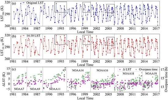
The primary objective of this work is to generate a long-term LST with the same local times from NOAA-AVHRR data. Therefore, we provide an example that illustrates how to estimate time series LSTs and present the effect of the ODC algorithm on a grassland pixel. The sample point is located in Hebei province with a center coordination of (114.3 °N, 41.1 °E), which is a transitional zone between the Inner Mongolian Plateau and the North China Plain. The input variables are the TOA brightness temperatures, VZA, viewing time, and NDVI, which can be directly extracted from AVH09C1 and AVH13C1. The emissivities, WVC, and LST are retrieved by applying the SWCVR method, the NDVI-based threshold method, and the improved GSW method, respectively. Subsequently, the influence of orbit drift on LST is removed by using the physically-based correction method. In consideration of the excessive amount of data, only the observations on the 10th, 20th, and 30th day of every month from 1981 to 2017 are used.
Figure 13 shows the results. Firstly, from subplot (a), one can see that the variation of LSTs at the sample point illustrates clear seasonal characteristics: LSTs in the summer are the highest, LSTs in winter are the lowest, and those in spring and autumn are in the middle. This phenomenon is consistent with a local temperate monsoon climate, which suggests that the refined GSW algorithm can obtain rational LSTs. However, as satellites operate, their overpass times become later and later. As Figure 13c shows, the maximum time drift can approach five hours; for example, the overpass times of NOAA-11 vary from 12:30 to 17:00. As a result, a “cooling trend” at the end of each satellite’s life-period, i.e., 1984, 1988, 1994, 2000, 2006, and 2013, can be observed from Figure 13a. In particular, there are obvious LST decreases for the periods from 1992 to 1994 and from 1999 to 2000, as well as from 2005 to 2006, i.e., three black rectangles in subplot (a). Fortunately, use of the proposed ODC algorithm can effectively reduce the influence of orbit drift. As shown in Figure 13b, the “cooling trend” in three black rectangles is significantly improved. Generally speaking, orbit drift correction is more meaningful at the end than at the beginning of the satellite operational cycle. Therefore, the corrected result is encouraging.
4. Discussion
Equation (2) is one of basic equations for the proposed orbit drift correction algorithm and it is also used to separate the vegetation and soil component temperatures. In a previous study [72], for component temperature estimation, besides the FVC retrieval error, the FVC type, i.e., FVC size and degree of change, also exerts important influence on the result. Specifically, vegetation/soil would have better performance with an increase/decrease in the FVC size, and both of them would achieve better performance with an increase in the change in the degree of FVC. Unlike the separation of component temperatures, soil and vegetation are the middle variables of LST at reference times in this work. For this reason, FVC size should not be a sensitive factor for the eventual result. Here, we only analyze the influence of the FVC change degree, since this factor can result in different correlations among the different pixels. The FVC standard deviation (STD) within a 3×3 neighboring area is selected as the index for the FVC change degree. Firstly, five cases of FVC STD are prescribed, which include (0, 0.1), (0.1, 0.2), (0.2, 0.3), (0.3, 0.4), and (0.4, 0.5). Subsequently, for each case, 100 different neighboring areas are simulated for performance evaluation. Similarly, only the data at 15:00 are used. As one can easily observe in Figure 14, the RMSEs of different FVC STDs are basically identical, which indicates that the influence of the FVC change degree on the correction result is slight. This result further suggests that the method for expressing the LST is not very important for the proposed orbit drift correction algorithm, whereas the application of the DTC model is the real key that ensures a satisfied correction effect. Therefore, our method is flexible and it can be updated by using other empirical and semi-empirical LST models, such as NDVI [73], NDVI and the digital elevation model (DEM) [74], and Albedo [75] to describe the LST.
Using neighboring information solves Equation (9), i.e., these five parameters are identical within a neighbor, since there is only one available NOAA-AVHRR observation per day. Here, the window size is set as 3 × 3, which has the highest computational efficiency on the premise of being solvable. If the original NOAA-AVHRR data rather than the LTDR products are used, the spatial resolution is 1 km. A higher spatial resolution might produce higher spatial heterogeneity. One may need to first identify similar pixels to ensure that the assumption of identical parameters is valid [59]. As a result, there may be fewer than five similar pixels in a 3 × 3 neighbor. To solve Equation (9), one can reduce the number of unknown parameters, such as by calculating while using the overpass time and geo-location of the pixel. However, expanding the window size to 5 × 5 or even larger is a more common method. In this case, the assumption of identical parameters would be more difficult to establish. A possible method is to consider the spatial correlation between the center pixel and other pixels in the neighbor [60] to balance the availability of the assumption and window size. One can also determine the best window size by analyzing the variation of the condition number of the coefficient matrix with respect to the window size [61].
The soil temperatures are distinct for different soil moisture conditions. Therefore, the assumption that soil temperatures of 3 × 3 pixels are invariant might be not feasible when soil moisture changes greatly. Although soil temperature is just a middle variable and the influence of its accuracy might be slight for the eventual correction result, it is necessary to assess the availability of the ODC algorithm for areas with different soil moisture conditions. The representativeness of the normalized LST for the actual LST at 14:30 is another limitation of this algorithm. The DTC model is a clear-sky model and it assumes that the surface radiative balance is under clear-sky conditions. However, local meteorology (e.g., wind) plays an important role in the overall surface energy balance. Therefore, although using the clear-sky filter method that is mentioned in Section 3.2.2 can identify cloudless moments, the validation of the ODC algorithm and the representativeness of the corrected LST still need be further analyzed.
5. Conclusions
We implemented a refined nonlinear GSW algorithm to retrieve the LSTs and developed a novel physical method based on the DTC model and a Bayesian optimization algorithm to correct the effect of orbit drift to produce a long-term global LST product with the same local time from time series NOAA-AVHRR.
Six-year NOAA-14 satellite data and multi-year SURFRAD measurements were used to evaluate the performance of our methods. In terms of LST retrieval, the RMSEs ranged from 4.1 K to 2.2 K and the overall Biases ranged from −0.4 K to 2.0 K over six sites, which suggested competitive accuracy when compared with current LST products. In addition, the influences of viewing angle and season were also analyzed and better performance was found under small zenith angles and during winter.
For the new ODC algorithm, observation time, LST at viewing time, and FVC were three important input variables. Analyses that were based on simulations indicated that this method had different correction accuracies for different viewing times. Specifically, the larger the time difference with the reference time, the worse the performance of the method. Moreover, LST retrieval errors significantly affected the correction errors, and these two errors had essentially identical change amplitudes. However, the corrected performance was less sensitive to the FVC, including its retrieval error and types, which suggests that the proposed method can be updated by applying other LST expressions. Furthermore, the validation with SURFRAD LSTs indicated that RMSE variations of LST estimations due to ODC were within ±0.5 K, suggesting an encouraging correction effect. This result also demonstrated that the LST retrieval accuracy had important influence on ODC performance, for which the correlation coefficients varied from 0.62 to 0.91.
Author Contributions
Conceptualization, X.L. and B.-H.T.; Formal analysis, G.Y.; Methodology, X.L., B.-H.T. and Z.-L.L.; Validation, S.L.; Writing—original draft, X.L.; Writing—review & editing, X.L., B.-H.T. and S.L.
Funding
This research was funded by the National Key Research and Development Program of China (2016YFA0600103), the National Natural Science Foundation of China (41571353 and 41871244), and the Innovation Project of LREIS (O88RA801YA). The work of X. L. was supported by the China Scholarship Council for his stay in ICube, France.
Acknowledgments
A preliminary version of this paper was presented at IEEE International Geoscience and Remote Sensing Symposium 2018 [55]. Our initial conference paper paid attention to the retrieval algorithm for LST using simulated dataset, and did not address the problem of orbit drift correction. This study addressed this issue and provided detailed analyses using in-situ data. NOAA-AVHRR data were downloaded from the website at https://ltdr.modaps.eosdis.nasa.gov/cgi-bin/ltdr/ltdrPage.cgi and SURFRAD data were downloaded from the FTP directory at ftp://aftp.cmdl.noaa.gov/data/radiation/surfrad/.
Conflicts of Interest
The authors declare no conflict of interest.
References
- Norman, J.M.; Becker, F. Terminology in thermal infrared remote sensing of natural surfaces. Remote. Sens. Rev. 1995, 12, 159–173. [Google Scholar] [CrossRef]
- Li, Z.-L.; Tang, B.-H.; Wu, H.; Ren, H.; Yan, G.; Wan, Z.; Trigo, I.F.; Sobrino, J.A. Satellite-derived land surface temperature: Current status and perspectives. Remote. Sens. Env. 2013, 131, 14–37. [Google Scholar] [CrossRef]
- Prata, A.; Caselles, V.; Coll, C.; Sobrino, J.; Ottle, C. Thermal remote sensing of land surface temperature from satellites: Current status and future prospects. Remote. Sens. Rev. 1995, 12, 175–224. [Google Scholar] [CrossRef]
- Vinnikov, K.Y.; Yu, Y.; Goldberg, M.D.; Tarpley, D.; Romanov, P.; Laszlo, I.; Chen, M. Angular anisotropy of satellite observations of land surface temperature. Geophys. Res. Lett. 2012, 39. [Google Scholar] [CrossRef]
- Qin, Z.; Karnieli, A.; Berliner, P. A mono-window algorithm for retrieving land surface temperature from Landsat TM data and its application to the Israel-Egypt border region. Int. J. Remote Sens. 2001, 22, 3719–3746. [Google Scholar] [CrossRef]
- Jiménez-Muñoz, J.C.; Sobrino, J.A. A generalized single-channel method for retrieving land surface temperature from remote sensing data. J. Geophys. Res. Atmos. 2003, 108. [Google Scholar] [CrossRef]
- Becker, F.; Li, Z.-L. Towards a local split window method over land surfaces. Remote Sens. 1990, 11, 369–393. [Google Scholar] [CrossRef]
- Wan, Z.; Dozier, J. A generalized split-window algorithm for retrieving land-surface temperature from space. IEEE Trans. Geosci. Remote Sens. 1996, 34, 892–905. [Google Scholar]
- Coll, C.; Caselles, V.; Sobrino, J.A.; Valor, E. On the atmospheric dependence of the split-window equation for land surface temperature. Remote Sens. 1994, 15, 105–122. [Google Scholar] [CrossRef]
- Gillespie, A.; Rokugawa, S.; Matsunaga, T.; Cothern, J.S.; Hook, S.; Kahle, A.B. A temperature and emissivity separation algorithm for Advanced Spaceborne Thermal Emission and Reflection Radiometer (ASTER) images. IEEE Trans. Geosci. Remote Sens. 1998, 36, 1113–1126. [Google Scholar] [CrossRef]
- Sobrino, J.; Sòria, G.; Prata, A. Surface temperature retrieval from Along Track Scanning Radiometer 2 data: Algorithms and validation. J. Geophys. Res. Atmos. 2004, 109. [Google Scholar] [CrossRef]
- Li, Z.-L.; Becker, F. Feasibility of land surface temperature and emissivity determination from AVHRR data. Remote Sens. Environ. 1993, 43, 67–85. [Google Scholar] [CrossRef]
- Wan, Z.; Li, Z.-L. A physics-based algorithm for retrieving land-surface emissivity and temperature from EOS/MODIS data. IEEE Trans. Geosci. Remote Sens. 1997, 35, 980–996. [Google Scholar]
- Wang, N.; Wu, H.; Nerry, F.; Li, C.; Li, Z.-L. Temperature and emissivity retrievals from hyperspectral thermal infrared data using linear spectral emissivity constraint. IEEE Trans. Geosci. Remote Sens. 2011, 49, 1291–1303. [Google Scholar] [CrossRef]
- Wan, Z. MODIS Land-Surface Temperature Algorithm Theoretical Basis Document (LST ATBD); Institute for Computational Earth System Science: Santa Barbara, CA, USA, 1999; Volume 75. [Google Scholar]
- Hulley, G.; Malakar, N.; Hughes, T.; Islam, T.; Hook, S. Moderate Resolution Imaging Spectroradiometer (MODIS) MOD21 Land Surface Temperature and Emissivity Algorithm Theoretical Basis Document; Jet Propulsion Laboratory, National Aeronautics and Space Administration: Pasadena, CA, USA, 2016.
- Prata, A. Land Surface Temperature Measurement from Space: AATSR Algorithm Theoretical Basis Document; Contract Report to ESA, CSIRO Atmospheric Research: Aspendale, Victoria, Australia, 2002; pp. 1–34. [Google Scholar]
- Gillespie, A.R.; Rokugawa, S.; Hook, S.J.; Matsunaga, T.; Kahle, A.B. Temperature/Emissivity Separation Algorithm Theoretical Basis Document, Version 2.4; ATBD Contract NAS5-31372; NASA: Washington, DC, USA, 1999.
- Hulley, G.; Islam, T.; Freepartner, R.; Malakar, N. Visible Infrared Imaging Radiometer Suite (VIIRS) Land Surface Temperature and Emissivity Product Collection 1 Algorithm Theoretical Basis Document; Jet Propulsion Laboratory, National Aeronautics and Space Administration: Pasadena, CA, USA, 2016.
- Baker, N.; Kilcoyne, H. Joint Polar Satellite System (JPSS) VIIRS Land Surface Temperature Algorithm Theoretical Basis Document; Goddard Space Flight Center: Greenbelt, MD, USA, 2011.
- Sun, D.; Fang, L.; Yu, Y. GOES LST Algorithm Theoretical Basis Document; NOAA NESDIS Center for Satellite Applications and Research: College Park, MD, USA, 2012.
- Trigo, I.; Freitas, S.; Bioucas-Dias, J.; Barroso, C.; Monteiro, I.; Viterbo, P. Algorithm Theoretical Basis Document for Land Surface Temperature (LST). LSA-4 (MLST); LSA SAF: Lisboa, Portugal, 2009. [Google Scholar]
- Ghent, D. Maximising the benefits of satellite LST within the user community: ESA DUE GlobTemperature. In AGU Fall Meeting Abstracts; American Geophysical Union: Washington, DC, USA, 2014; Available online: http://adsabs.harvard.edu/abs/2014AGUFMGC53E.01G (accessed on 21 October 2019).
- IPCC. Contribution of Working Groups I, II and III to the Fifth Assessment Report of the Intergovernmental Panel on Climate Change; CoreWriting Team, Pachauri, R.K., Meyer, L.A., Eds.; Climate Change 2014: Synthesis Report; IPCC: Geneva, Switzerland, 2014; p. 151. [Google Scholar]
- Sobrino, J.; Raissouni, N. Toward remote sensing methods for land cover dynamic monitoring: Application to Morocco. Int. J. Remote Sens. 2000, 21, 353–366. [Google Scholar] [CrossRef]
- Pinheiro, A.C.T.; Mahoney, R.; Privette, J.L.; Tucker, C.J. Development of a daily long term record of NOAA-14 AVHRR land surface temperature over Africa. Remote Sens. Environ. 2006, 103, 153–164. [Google Scholar] [CrossRef]
- Frey, C.; Kuenzer, C.; Dech, S. Assessment of Mono- and Split-Window Approaches for Time Series Processing of LST from AVHRR—A TIMELINE Round Robin. Remote Sens. 2017, 9, 72. [Google Scholar] [CrossRef]
- Zhou, J.; Liang, S.; Cheng, J.; Wang, Y.; Ma, J. The GLASS land surface temperature product. IEEE J. Sel. Top. Appl. Earth Obs. Remote Sens. 2019, 12, 493–507. [Google Scholar] [CrossRef]
- Price, J.C. Timing of NOAA afternoon passes. Int. J. Remote Sens. 1991, 12, 193–198. [Google Scholar] [CrossRef]
- Gutman, G. On the monitoring of land surface temperatures with the NOAA/AVHRR: Removing the effect of satellite orbit drift. Int. J. Remote Sens. 1999, 20, 3407–3413. [Google Scholar] [CrossRef]
- Gleason, A.C.; Prince, S.D.; Goetz, S.J.; Small, J. Effects of orbit drift on land surface temperature measured by AVHRR thermal sensors. Remote Sens. Environ. 2002, 79, 147–165. [Google Scholar] [CrossRef]
- Sobrino, J.A.; Julien, Y.; Atitar, M.; Nerry, F. NOAA-AVHRR orbit drift correction from solar zenithal angle data. IEEE Trans. Geosci. Remote Sens. 2008, 46, 4014–4019. [Google Scholar] [CrossRef]
- Julien, Y.; Sobrino, J.A. Correcting AVHRR Long Term Data Record V3 estimated LST from orbit drift effects. Remote Sens. Environ. 2012, 123, 207–219. [Google Scholar] [CrossRef]
- Jin, M.; Treadon, R. Correcting the orbit drift effect on AVHRR land surface skin temperature measurements. Int. J. Remote Sens. 2003, 24, 4543–4558. [Google Scholar] [CrossRef]
- Sobrino, J.A.; Julien, Y. Time series corrections and analyses in thermal remote sensing. In Thermal Infrared Remote Sensing; Springer: Berlin/Heidelberg, Germany, 2018; pp. 267–285. [Google Scholar]
- Pedelty, J.; Devadiga, S.; Masuoka, E.; Brown, M.; Pinzon, J.; Tucker, C.; Vermote, E.; Prince, S.; Nagol, J.; Justice, C. Generating a long-term land data record from the AVHRR and MODIS instruments. In Proceedings of the Geoscience and Remote Sensing Symposium, IGARSS 2007, Barcelona, Spain, 23–28 July 2007. [Google Scholar]
- Inamdar, A.K.; French, A.; Hook, S.; Vaughan, G.; Luckett, W. Land surface temperature retrieval at high spatial and temporal resolutions over the southwestern United States. J. Geophys. Res. Atmos. 2008, 113. [Google Scholar] [CrossRef]
- Duan, S.-B.; Li, Z.-L.; Wang, N.; Wu, H.; Tang, B.-H. Evaluation of six land-surface diurnal temperature cycle models using clear-sky in situ and satellite data. Remote Sens. Environ. 2012, 124, 15–25. [Google Scholar] [CrossRef]
- Sobrino, J.A.; Jiménez-Muñoz, J.C.; Sòria, G.; Romaguera, M.; Guanter, L.; Moreno, J.; Plaza, A.; Martínez, P. Land surface emissivity retrieval from different VNIR and TIR sensors. IEEE Trans. Geosci. Remote Sens. 2008, 46, 316–327. [Google Scholar] [CrossRef]
- Quan, J.; Chen, Y.; Zhan, W.; Wang, J.; Voogt, J.; Li, J. A hybrid method combining neighborhood information from satellite data with modeled diurnal temperature cycles over consecutive days. Remote Sens. Environ. 2014, 155, 257–274. [Google Scholar] [CrossRef]
- Goodrum, G.; Kidwell, K.B.; Winston, W.; Aleman, R. NOAA KLM User’s Guide. 1999. Available online: http://webapp1.dlib.indiana.edu/virtual_disk_library/index.cgi/2790181/FID3711/klm/index.htm (accessed on 26 September 2019).
- Kidwell, K. NOAA Polar Orbiter Data (POD) User’s Guide, November 1998 Revision; National Climatic Data Center: Asheville, NC, USA; NESDIS: Silver Spring, MD, USA; NOAA: Silver Spring, MD, USA, 1998.
- Wang, W.; Liang, S.; Meyers, T. Validating MODIS land surface temperature products using long-term nighttime ground measurements. Remote. Sens. Environ. 2008, 112, 623–635. [Google Scholar] [CrossRef]
- Li, S.; Yu, Y.; Sun, D.; Tarpley, D.; Zhan, X.; Chiu, L. Evaluation of 10 year AQUA/MODIS land surface temperature with SURFRAD observations. Int. J. Remote Sens. 2014, 35, 830–856. [Google Scholar] [CrossRef]
- Duan, S.-B.; Li, Z.-L.; Li, H.; Göttsche, F.-M.; Wu, H.; Zhao, W.; Leng, P.; Zhang, X.; Coll, C. Validation of Collection 6 MODIS land surface temperature product using in situ measurements. Remote Sens. Environ. 2019, 225, 16–29. [Google Scholar] [CrossRef]
- Martin, M.; Ghent, D.; Pires, A.; Göttsche, F.-M.; Cermak, J.; Remedios, J. Comprehensive in Situ Validation of Five Satellite Land Surface Temperature Data Sets over Multiple Stations and Years. Remote Sens. 2019, 11, 479. [Google Scholar] [CrossRef]
- Wang, K.; Liang, S. Evaluation of ASTER and MODIS land surface temperature and emissivity products using long-term surface longwave radiation observations at SURFRAD sites. Remote Sens. Environ. 2009, 113, 1556–1565. [Google Scholar] [CrossRef]
- Ghent, D.; Corlett, G.; Göttsche, F.M.; Remedios, J. Global Land Surface Temperature From the Along-Track Scanning Radiometers. J. Geophys. Res. Atmos. 2017, 122, 12–67. [Google Scholar] [CrossRef] [Green Version]
- Guillevic, P.C.; Biard, J.C.; Hulley, G.C.; Privette, J.L.; Hook, S.J.; Olioso, A.; Göttsche, F.M.; Radocinski, R.; Román, M.O.; Yu, Y. Validation of Land Surface Temperature products derived from the Visible Infrared Imaging Radiometer Suite (VIIRS) using ground-based and heritage satellite measurements. Remote Sens. Environ. 2014, 154, 19–37. [Google Scholar] [CrossRef]
- Liu, Y.; Yu, Y.; Yu, P.; Göttsche, F.; Trigo, I. Quality assessment of S-NPP VIIRS land surface temperature product. Remote Sens. 2015, 7, 12215–12241. [Google Scholar] [CrossRef] [Green Version]
- Tang, B.-H.; Wu, H.; Li, C.; Li, Z.-L. Estimation of broadband surface emissivity from narrowband emissivities. Opt. Express 2011, 19, 185–192. [Google Scholar] [CrossRef]
- Cheng, J.; Liang, S.; Yao, Y.; Zhang, X. Estimating the optimal broadband emissivity spectral range for calculating surface longwave net radiation. IEEE Geosci. Remote Sens. Lett. 2012, 10, 401–405. [Google Scholar] [CrossRef]
- Wan, Z. New refinements and validation of the collection-6 MODIS land-surface temperature/emissivity product. Remote Sens. Environ. 2014, 140, 36–45. [Google Scholar] [CrossRef]
- Tang, B.-H. Nonlinear split-window algorithms for estimating land and sea surface temperatures from simulated chinese gaofen-5 satellite data. IEEE Trans. Geosci. Remote. Sens. 2018, 56, 6280–6289. [Google Scholar] [CrossRef]
- Liu, X.; Tang, B.-H.; Li, Z.-L. A Refined Generalized Split-Window Algorithm for Retrieving Long-Term Global Land Surface Temperature from Series NOAA-AVHRR Data. In Proceedings of the International Geoscience and Remote Sensing Symposium, IGARSS 2018, Valencia, Spain, 22–27 July 2018. [Google Scholar]
- Li, Z.-L.; Jia, L.; Su, Z.; Wan, Z.; Zhang, R. A new approach for retrieving precipitable water from ATSR2 split-window channel data over land area. Int. J. Remote Sens. 2003, 24, 5095–5117. [Google Scholar] [CrossRef]
- Tang, B.-H.; Shao, K.; Li, Z.-L.; Wu, H.; Tang, R. An improved NDVI-based threshold method for estimating land surface emissivity using MODIS satellite data. Int. J. Remote Sens. 2015, 36, 4864–4878. [Google Scholar] [CrossRef]
- Tang, B.-H.; Bi, Y.; Li, Z.-L.; Xia, J. Generalized split-window algorithm for estimate of land surface temperature from Chinese geostationary FengYun meteorological satellite (FY-2C) data. Sensors 2008, 8, 933–951. [Google Scholar] [CrossRef] [PubMed] [Green Version]
- Quan, J.; Zhan, W.; Ma, T.; Du, Y.; Guo, Z.; Qin, B. An integrated model for generating hourly Landsat-like land surface temperatures over heterogeneous landscapes. Remote Sens. Environ. 2018, 206, 403–423. [Google Scholar] [CrossRef]
- Zhan, W.; Chen, Y.; Zhou, J.; Li, J. An algorithm for separating soil and vegetation temperatures with sensors featuring a single thermal channel. Ieee Trans. Geosci. Remote Sens. 2011, 49, 1796–1809. [Google Scholar] [CrossRef]
- Liu, Q.; Yan, C.; Xiao, Q.; Yan, G.; Fang, L. Separating vegetation and soil temperature using airborne multiangular remote sensing image data. Int. J. Appl. Earth Obs. Geoinf. 2012, 17, 66–75. [Google Scholar] [CrossRef]
- Kallel, A.; Ottlé, C.; Le Hegarat-Mascle, S.; Maignan, F.; Courault, D. Surface temperature downscaling from multiresolution instruments based on Markov models. IEEE Trans. Geosci. Remote Sens. 2013, 51, 1588–1612. [Google Scholar] [CrossRef]
- Li, Z.-L.; Stoll, M.; Zhang, R.; Jia, L.; Su, Z. On the separate retrieval of soil and vegetation temperatures from ATSR data. Sci. China Ser. D Earth Sci. 2001, 44, 97–111. [Google Scholar]
- Jia, L.; Li, Z.-L.; Menenti, M.; Su, Z.; Verhoef, W.; Wan, Z. A practical algorithm to infer soil and foliage component temperatures from bi-angular ATSR-2 data. Int. J. Remote Sens. 2003, 24, 4739–4760. [Google Scholar] [CrossRef]
- Zhang, R.; Sun, X.; Wang, W.; Xu, J.; Zhu, Z.; Tian, J. An operational two-layer remote sensing model to estimate surface flux in regional scale: Physical background. Sci. China Ser. D 2005, 48, 225–244. [Google Scholar]
- Patil, A.; Huard, D.; Fonnesbeck, C.J. PyMC: Bayesian stochastic modelling in Python. J. Stat. Softw. 2010, 35, 1. [Google Scholar] [CrossRef] [PubMed] [Green Version]
- Newville, M.; Stensitzki, T.; Allen, D.B.; Rawlik, M.; Ingargiola, A.; Nelson, A. LMFIT: Non-linear least-square minimization and curve-fitting for Python. Astrophys. Source Code Libr. 2016. [Google Scholar] [CrossRef]
- Göttsche, F.-M.; Olesen, F.-S.; Bork-Unkelbach, A. Validation of land surface temperature derived from MSG/SEVIRI with in situ measurements at Gobabeb, Namibia. Int. J. Remote Sens. 2013, 34, 3069–3083. [Google Scholar] [CrossRef]
- Davies, L.; Gather, U. The identification of multiple outliers. J. Am. Stat. Assoc. 1993, 88, 782–792. [Google Scholar] [CrossRef]
- Tang, B.; Li, Z.-L. Estimation of instantaneous net surface longwave radiation from MODIS cloud-free data. Remote Sens. Environ. 2008, 112, 3482–3492. [Google Scholar] [CrossRef]
- Jiang, Y.; Jiang, X.-G.; Tang, R.; Li, Z.-L.; Zhang, Y.; Liu, Z.-X.; Huang, C. Effect of Cloud Cover on Temporal Upscaling of Instantaneous Evapotranspiration. J. Hydrol. Eng. 2018, 23, 05018002. [Google Scholar] [CrossRef]
- Zhao, W.; Li, A.; Li, Z.-L. Component Temperature Estimation from Simulated Geostationary Meteorological Satellite Data Based on MAP Criterion and Markov Models. J. Geo-Inf. Sci. 2013, 15, 422–430. (In Chinese) [Google Scholar] [CrossRef]
- Agam, N.; Kustas, W.P.; Anderson, M.C.; Li, F.; Neale, C.M. A vegetation index based technique for spatial sharpening of thermal imagery. Remote Sens. Environ. 2007, 107, 545–558. [Google Scholar] [CrossRef]
- Duan, S.-B.; Li, Z.-L. Spatial downscaling of MODIS land surface temperatures using geographically weighted regression: Case study in Northern China. IEEE Trans. Geosci. Remote Sens. 2016, 54, 6458–6469. [Google Scholar] [CrossRef]
- Song, L.; Liu, S.; Kustas, W.P.; Zhou, J.; Ma, Y. Using the surface temperature-albedo space to separate regional soil and vegetation temperatures from ASTER data. Remote Sens. 2015, 7, 5828–5848. [Google Scholar] [CrossRef] [Green Version]
Figure 1.
Equatorial Crossing Time (ECT) for National Oceanic and Atmospheric Administration (NOAA) afternoon Satellites (Adapted from https://www.star.nesdis.noaa.gov/smcd/emb/vci/VH/vh_avhrr_ect.php).
Figure 1.
Equatorial Crossing Time (ECT) for National Oceanic and Atmospheric Administration (NOAA) afternoon Satellites (Adapted from https://www.star.nesdis.noaa.gov/smcd/emb/vci/VH/vh_avhrr_ect.php).

Figure 2.
Schematic diagram of the diurnal temperature cycle (DTC) model [Adapted from Duan et al. [38].
Figure 2.
Schematic diagram of the diurnal temperature cycle (DTC) model [Adapted from Duan et al. [38].

Figure 3.
Spectral Response Functions of advanced very high resolution radiometer (AVHRR) Sensors.

Figure 4.
The result of the orbit drift correction for (a) the entire interval and (b–h) different moments. The subscript ‘Ori’ represents the simulated land surface temperatures (LSTs) at the original viewing time, and ‘ODC’ represents the corrected LSTs at 14:30, estimated from the corresponding time. The solid line represents 1:1, the two dashed lines are 1:1 ± 3 K, and the two dashdot lines are 1:1 ± 5 K.

Figure 5.
Sensitivity of the physically-based orbit drift correction algorithm for LST retrieval error.
Figure 5.
Sensitivity of the physically-based orbit drift correction algorithm for LST retrieval error.

Figure 6.
Sensitivity of the physically-based orbit drift correction algorithm to fractional vegetation cover (FVC) retrieval error.
Figure 6.
Sensitivity of the physically-based orbit drift correction algorithm to fractional vegetation cover (FVC) retrieval error.

Figure 7.
Scatterplots of the retrieved NOAA-14 LST versus the in-situ SURFRAD LST for all matched days over (a) Bondville (BND), (b) Table Mountain (TBL), (c) Desert Rock (DRA), (d) Fort Peck (FPK), (e) Goodwin Creek (GWN), and (f) Pennsylvania State University (PSU).
Figure 7.
Scatterplots of the retrieved NOAA-14 LST versus the in-situ SURFRAD LST for all matched days over (a) Bondville (BND), (b) Table Mountain (TBL), (c) Desert Rock (DRA), (d) Fort Peck (FPK), (e) Goodwin Creek (GWN), and (f) Pennsylvania State University (PSU).

Figure 8.
Scatterplots of the retrieved NOAA-14 LST at different VZA sub-groups versus the in-situ SURFRAD LST over (a) BND, (b) TBL, (c) DRA, (d) FPK, (e) GWN, and (f) PSU.
Figure 8.
Scatterplots of the retrieved NOAA-14 LST at different VZA sub-groups versus the in-situ SURFRAD LST over (a) BND, (b) TBL, (c) DRA, (d) FPK, (e) GWN, and (f) PSU.

Figure 9.
Seasonal root-mean-square error (RMSE) and Bias of the retrieved NOAA-14 LST over (a) BND, (b) TBL, (c) DRA, (d) FPK, (e) GWN, and (f) PSU.
Figure 9.
Seasonal root-mean-square error (RMSE) and Bias of the retrieved NOAA-14 LST over (a) BND, (b) TBL, (c) DRA, (d) FPK, (e) GWN, and (f) PSU.

Figure 10.
Scatterplots of the retrieved NOAA-14 LST versus the in-situ SURFRAD LST for days in which the sky is cloudless at 14:30 over (a) BND, (b) TBL, (c) DRA, (d) FPK, (e) GWN, and (f) PSU.
Figure 10.
Scatterplots of the retrieved NOAA-14 LST versus the in-situ SURFRAD LST for days in which the sky is cloudless at 14:30 over (a) BND, (b) TBL, (c) DRA, (d) FPK, (e) GWN, and (f) PSU.

Figure 11.
The results of orbit drift correction over (a) BND, (b) TBL, (c) DRA, (d) FPK, (e) GWN, and (f) PSU. The abbreviation ‘Ori’ represents the retrieved LSTs at the original viewing time, and ‘ODC’ represents the corrected LSTs at 14:30, as estimated from the corresponding time.
Figure 11.
The results of orbit drift correction over (a) BND, (b) TBL, (c) DRA, (d) FPK, (e) GWN, and (f) PSU. The abbreviation ‘Ori’ represents the retrieved LSTs at the original viewing time, and ‘ODC’ represents the corrected LSTs at 14:30, as estimated from the corresponding time.

Figure 12.
Scatterplots of the ΔLST (retrieved NOAA LST–in-situ SURFRAD LST) at the original viewing time versus ΔLST (corrected NOAA LST–in-situ SURFRAD LST) at 14:30 over (a) BND, (b) TBL, (c) DRA, (d) FPK, (e) GWN, and (f) PSU.
Figure 12.
Scatterplots of the ΔLST (retrieved NOAA LST–in-situ SURFRAD LST) at the original viewing time versus ΔLST (corrected NOAA LST–in-situ SURFRAD LST) at 14:30 over (a) BND, (b) TBL, (c) DRA, (d) FPK, (e) GWN, and (f) PSU.

Figure 13.
The LSTs over a grassland pixel (114.3 °N, 41.1 °E) from 1981 to 2017. (a) the original LST at overpass time using the improved GSW algorithm; (b) the corrected LST at 14:30 while using the proposed ODC algorithm; and, (c) the ΔLST (corrected LST at 14:30–original LST at overpass time) and the corresponding overpass time. The three black rectangles, from left to right, are the LSTs from 1992 to 1994, LSTs from 1999 to 2000, and LSTs from 2005 to 2006, respectively.

Figure 14.
The influence of FVC standard deviation (STD) on the physically-based orbit drift correction algorithm.
Figure 14.
The influence of FVC standard deviation (STD) on the physically-based orbit drift correction algorithm.


Table 1.
Specification of Surface Radiation Budget Network (SURFRAD) Stations.
| Station Name | Lon (°W) | Lat (°N) | Elevation (m) | Installed Time | Land Cover Type | Broadband Emissivity |
|---|---|---|---|---|---|---|
| BND | 88.373 | 40.051 | 230 | April 1994 | Cropland | 0.968 |
| TBL | 105.238 | 40.126 | 1689 | July 1995 | Bare soil | 0.972 |
| DRA | 116.020 | 36.623 | 1007 | March 1998 | Bare soil | 0.967 |
| FPK | 105.102 | 48.308 | 634 | November 1994 | Grassland | 0.973 |
| GWN | 89.873 | 34.255 | 98 | December 1994 | Grassland | 0.971 |
| PSU | 77.931 | 40.720 | 376 | June 1998 | Cropland | 0.970 |
BND: Bondville, TBL: Table Mountain, DRA: Desert Rock, FPK: Fort Peck, GWN: Goodwin Creek, PSU: Pennsylvania State University.
Table 2.
The Initial Value and Valid Range of Each Parameter of Equation (9).
| Parameter | Initial Value | Minimum | Maximum |
|---|---|---|---|
| (K) | LST | LST-30 | LST+20 |
| (K) | LST | LST-20 | LST+30 |
| (K) | 20 | 5 | 30 |
| (h) | 13 | 10 | 16 |
| (h) | 13 | 12 | 15 |
LST is the temperature at the observation time.
© 2019 by the authors. Licensee MDPI, Basel, Switzerland. This article is an open access article distributed under the terms and conditions of the Creative Commons Attribution (CC BY) license (http://creativecommons.org/licenses/by/4.0/).
Share and Cite
MDPI and ACS Style
Liu, X.; Tang, B.-H.; Yan, G.; Li, Z.-L.; Liang, S. Retrieval of Global Orbit Drift Corrected Land Surface Temperature from Long-term AVHRR Data. Remote Sens. 2019, 11, 2843. https://doi.org/10.3390/rs11232843
AMA Style
Liu X, Tang B-H, Yan G, Li Z-L, Liang S. Retrieval of Global Orbit Drift Corrected Land Surface Temperature from Long-term AVHRR Data. Remote Sensing. 2019; 11(23):2843. https://doi.org/10.3390/rs11232843
Chicago/Turabian StyleLiu, Xiangyang, Bo-Hui Tang, Guangjian Yan, Zhao-Liang Li, and Shunlin Liang. 2019. "Retrieval of Global Orbit Drift Corrected Land Surface Temperature from Long-term AVHRR Data" Remote Sensing 11, no. 23: 2843. https://doi.org/10.3390/rs11232843
Note that from the first issue of 2016, this journal uses article numbers instead of page numbers. See further details here.