Benchmarking Machine Learning Algorithms for Instantaneous Net Surface Shortwave Radiation Retrieval Using Remote Sensing Data


1
State Key Laboratory of Resources and Environment Information System, Institute of Geographic Sciences and Natural Resources Research, Chinese Academy of Sciences, Beijing 100101, China
2
University of Chinese Academy of Sciences, Beijing 100049, China
3
Jiangsu Center for Collaborative Innovation in Geographical Information Resource Development and Application, Nanjing 210023, China
*
Author to whom correspondence should be addressed.
Remote Sens. 2019, 11(21), 2520; https://doi.org/10.3390/rs11212520
Submission received: 9 September 2019
/
Revised: 24 October 2019
/
Accepted: 26 October 2019
/
Published: 28 October 2019
(This article belongs to the Special Issue Remote Sensing of Land Surface Radiation Budget)
Abstract
:Net surface shortwave radiation (NSSR) is one of the most important fundamental parameters in various land processes. Benefiting from its efficient nonlinear fitting ability, machine learning algorithms have a great potential in the retrieval of NSSR. However, few studies have explored the level of accuracy that machine learning algorithms can reach for different land covers on the worldwide scale and what the optimal independent variables are in the machine learning-based NSSR model. To guide the use of machine learning algorithms correctly in the retrieval of NSSR, it is necessary to give a comprehensive analysis from algorithm complexity, accuracy, and other aspects. In this study, three classic machine learning algorithms, including Random Forest (RF), Artificial Neural Network (ANN), and Support Vector Regression (SVR), were built well to estimate instantaneous NSSR with optimal hyperparameters by elaborately selecting different independent variables, including top of atmosphere (TOA) channel spectral reflectance, geographic parameters, surface information, and atmosphere conditions. Global FLUXNET in situ measurements throughout 2014 were used to validate the accuracies of retrieved NSSR over various land cover types. The root mean square error (RMSE) is below 55 W/m2, and the distributions of error histogram are also similar. Approximately 50% of absolute error were within 25 W/m2. There was a performance difference of NSSR estimations in various surface types, and the performance of three machine learning methods in a specific surface type was also different. However, the RF method may be considered as the optimal methodology to retrieve NSSR from MODIS data, owing to its relatively better precision and concise hyperparameter-tuned process. The importance analysis of the proposed independent variables of NSSR retrieval shows that the introduction of geographic information can effectively reduce the error of NSSR retrieval, and surface information and atmosphere information are not necessary. It was also found that a combination of geographic information and blue band TOA reflectance already have a pretty good accuracy in NSSR retrieval, which implies there is a possibility to transfer our NSSR model to other satellite sensors, especially with insufficient channels. In a word, the NSSR model with machine learning algorithms would be an efficient, concise, and general method in the future.
1. Introduction
Net surface radiation characterizes the surface radiation budget and plays a critical role in ecological, physical, biogeochemical, and hydrological processes [1,2]. As the main component of net surface radiation, net surface shortwave radiation (NSSR) is calculated as the difference between surface incident shortwave radiation and the amount of radiation reflected back into the atmosphere by the surface [3] and represents the amount of solar radiation absorbed by the surface. Therefore, the ability to better monitor instantaneous NSSR globally is essential to better understand existing feedbacks between the surface energy cycles and the effects of climate change [4]. It is widely recognized that remote sensing technology from the satellite is a convenient and effective method to study Earth sciences, including surface radiation balance, ecosystem dynamics, and climate change [5,6,7]. Thus, reliable global NSSR retrieval from satellite remote sensing data at a high spatial and temporal resolution is required.
In recent years, traditional approaches of retrieving NSSR from satellite data have involved statistical/empirical approaches, physically-based approaches, and mixed approaches [3]. The aim of statistical/empirical approaches is to establish the statistical/empirical relationship between measured NSSR and observations at the top of atmosphere (TOA) directly [8,9,10]. Specifically, Pinker and Corio [9] made direct estimations of NSSR using NOAA5 satellite data, finding that a high correlation exists between TOA observations and in situ NSSR. However, the physically-based methods consider the complete radiative transfer process with satellite-retrieved physical properties of the surface, atmosphere, and geometric optics [11,12,13]. For example, the NSSR can be successfully retrieved by introducing parameterization of the absorption and scattering effects of water vapor, cloud, and aerosol in the atmosphere [12]. The mixed approaches combine the statistical/empirical method with the physically-based method, which are widely used for estimating instantaneous NSSR in the field of traditional approaches [5,14,15]. For instance, based on numerous moderate resolution atmospheric transmission model (MODTRAN) simulations of various atmosphere and geographic conditions, Tang [15] built the NSSR model from the moderate resolution imaging spectroradiometer (MODIS) data on the Terra platform by introducing the least square method in the fitting of the relationship of TOA observations and ground NSSR. However, these traditional methods usually apply numerous specific formulas, which may not have good representations of real interactions. Many coefficients of formulas should be fitted, which are always limited by the initial values with the iterative solution algorithm. In addition, atmosphere conditions (clear sky or cloudy sky) should usually be distinguished in traditional approaches [5,15,16], leading to the high complexity of the NSSR retrieval model. Consequently, concise and accurate approaches with the latest methodologies for generating instantaneous NSSR are needed.
Generally, the NSSR is a nonlinear function of spectral information, surface properties, atmosphere conditions, and geographic parameters [4,5,14,17,18]. Nowadays, machine learning algorithms are widely used in remote sensing retrievals with the regression mission, due to its powerful ability of adaptive nonlinear fitting [19]. Machine learning algorithms can automatically learn and organize the recognition of inner data patterns, without prespecifying the specific type of relationship between dependent and independent variables [20]. In NSSR retrieval applications, the variables of satellite channel reflectance [17,21,22], geographic parameters [17,21,22], atmosphere precipitable water [17], cloud information [21,23], surface properties [23], and other auxiliary data are universally regarded as independent variables. Note that the accuracy of these studies with machine learning methods is usually better than that of traditional methods. However, such research was usually based on a simulated dataset or on a few in situ observations, leading to a worse generalization of the NSSR model [17,21,22]. Some research applied ground auxiliary measurements or poor available data as independent variables of the NSSR model [23], causing the difficulty of acquisition of global NSSR. Few studies researched the different performance of NSSR retrieval using machine learning algorithms on various surface types, and the importance of variables affecting NSSR and the necessary variable are not provided. Thus, the machine learning algorithm for retrieving NSSR, having a better generalization ability, better global promotion, and better accuracy, is expected.
The purpose of this study is to explore the level of accuracy machine learning algorithms can reach for different land covers worldwide, and what the optimal independent variables are in the machine learning-based instantaneous NSSR model. Here, three classic machine learning algorithms, including Random Forest (RF), Artificial Neural Network (ANN), and Support Vector Regression (SVR), were used to build the NSSR model. MODIS remote sensing data were chosen as the drive sources of the NSSR model because they have a relatively high temporal and spatial resolution and there are various easy-available global products, including fundamental observations, land products, and atmosphere products [24]. Global FLUXNET in situ data of various surface types were used to evaluate the accuracy of the proposed NSSR model. Our study gives a detailed analysis of the performance of the machine learning-based NSSR models on different surface types; the importance and optimal combination of independent variables affecting NSSR were also analyzed.
2. Materials and Methods
2.1. Data
2.1.1. In Situ Data
FLUXNET is a network of globally distributed micrometeorological tower sites that measure turbulent flux, carbon dioxide, and water vapor exchange between terrestrial ecosystems and the atmosphere, using the eddy covariance method [25]. The flux measurement sites are linked across a confederation of regional networks in America (AmeriFlux), Europe (EuroFlux), Asia (AsiaFlux), Australia (OzFlux), and so on [26]. The FLUXNET community has harmonized, standardized, and gap-filled these regional networks to create the latest dataset, FLUXNET2015 Dataset [27], which contains the measurements of 212 sites. Some sites provide observations at a half-hourly temporal resolution, and some stations provide hourly observations [28].
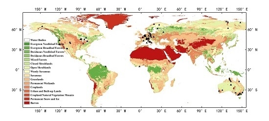
In our study, a total of 95 tower sites, which have effective observations from throughout 2014, were selected. Figure 1 shows the distribution of those aforementioned observing sites, and these sites represent a variety of surface types, ecosystem conditions, climate characters, and geographic environments. The proposed NSSR models will be evaluated by observations of these sites. However, these sites are mostly distributed in Europe, North America, and Australia. Their representability may be relatively limited considering the variation of the climate and ground surface condition. The distribution of land cover types is also shown on the map, which is defined by the International Geosphere-Biosphere Programme (IGBP) [29]. Here, the MCD12C1 product, provided by the United States Geological Survey [30], was used to acquire the distribution of global IGBP land cover types. The classification classes and description of land cover types are introduced in Table 1, and it can be found that the 95 selected sites cover 12 kinds of surface types. There are 19 sites of evergreen needleleaf forests (ENF), 9 sites of evergreen broadleaf forests (EBF), 1 site of deciduous needleleaf forests (DNF), 11 sites of deciduous broadleaf forests (DBF), 6 sites of mixed forests (MF), 1 site of closed shrublands (CSH), 4 sites of open shrublands (OSH), 4 sites of woody savannas (WSA), 4 sites of savannas (SAV), 14 sites of grasslands (GRA), 12 sites of permanent wetlands (WET), and 10 sites of croplands (CRO).
The FLUXNET2015 dataset has over 200 variables—among them, measured data, derived data, quality flags, uncertainty quantification variables, and results from intermediate data processing steps [31]. The measured data include flux energy (shortwave radiation, longwave radiation, latent heat, sensible heat), meteorological factors (air temperature, precipitation, specific humidity), and many auxiliary data. The NSSR of tower sites can be calculated as the difference between measured incoming shortwave radiation and measured outgoing shortwave radiation at the surface.
2.1.2. Remote Sensing Data
The first MODIS instrument, with a 10:30 equatorial crossing time, was launched aboard Terra in 1999, providing the MOD Series products; the second MODIS instrument, with a 13:30 equatorial crossing time, was launched aboard the Aqua platform in 2002, providing the MYD Series products [32,33]. Both Terra- and Aqua-MODIS instruments view the entire Earth’s surface every 1 to 2 days, acquiring radiance of 36 spectral bands in wavelengths from 0.405 to 14.385 µm at three spatial resolutions—250, 500, and 1000 m. Note that observations of first 7 spectral bands are usually used to estimate NSSR, which consists of a red band (0.620–0.670 µm), a near-infrared band (NIR, 0.841–0.876 µm), a blue band (0.459–0.479 µm), a green band (0.545–0.565 µm), and three shortwave infrared bands (SWIR, 1.230–1.250; 1.628–1.652; and 2.105–2.155 µm) [34]. MODIS instrument observations are produced by the National Aeronautics and Space Administration (NASA), providing various products about global dynamics and processes occurring on the land and in the lower atmosphere [35,36]. The twin-MODIS products can contribute to a range of Earth science areas, including Surface radiation balance, ecosystem dynamics, and agriculture studies.
In our study, both MOD series products and MYD series products were obtained to ensure the dataset size of NSSR machine learning application. Taking MOD series product as an example, MOD02, MOD03, MOD05, MOD09, and MOD35 images passing through the selected 95 sites were downloaded throughout 2014 [37]. For surface sites with a half-hourly temporal resolution, the time gap between the in-situ observations and satellite data is 15 min. For sites with an hourly temporal resolution, on the other hand, the time gap is 30 min. The MOD02 product provides calibrated and geolocated TOA spectral radiance of MODIS channels, and TOA spectral reflectance of solar reflective bands are also offered. The geolocation fields, including latitude, longitude, viewing zenith angle (VZA), and solar zenith angle (SZA) can be acquired in the MOD03 product; the atmosphere precipitable water product (MOD05) consists of column water–vapor amounts, applying a near-infrared algorithm; the MOD09 product provides an estimate of the surface spectral reflectance as it would be measured at ground level in the absence of atmospheric scattering or absorption, including the first 7 channels of MODIS. The MODIS cloud mask product (MOD35) assigns 4 clear-sky confidence levels (confident clear, probably clear, uncertain clear, cloudy) to each pixel in a remote sensing image, with the algorithm employing a series of visible and infrared threshold and consistency tests to specify confidence.
Specifically, the spatial resolution of MOD02, MOD03, MOD05, and MOD35 products is around 1 km, and these products provide instantaneous observations. Different from the above products, the spatial resolution of the MOD09 product used is around 0.05 degrees, and the temporal resolution is daily. In addition, the MCD12C1 product was used to acquire the IGBP surface type of selected sites and map the distribution of global IGBP land cover types in 2014.
2.2. Methodology
2.2.1. Net Surface Shortwave Radiation Retrieval Methodology
Generally, the relationship between NSSR and its independent variables (channel reflectance, geographic information, surface information, and atmosphere information) can be expressed by the following formula:
where function f represents the nonlinear relationship between dependent variable NSSR and its independent variables. Machine learning methods are essentially used to fit this nonlinear relationship, i.e., to develop an instantaneous NSSR retrieval model with various MODIS data.
Figure 2 shows the flowchart of net surface shortwave radiation retrieval methodology, and it can be found that the reflectance of MODIS’ first 7 spectral bands at TOA level (R1–R7), latitude (LAT), VZA, SZA, atmosphere precipitable water (w), the reflectance of MODIS first 7 spectral bands at surface level (SR1–SR7), and cloud mask (4 clear-sky confidence levels: CM1–CM4) are regarded as independent variables. Note that machine learning methods can acquire richer atmospheric information through the difference between the TOA channel reflectance and surface channel reflectance. More surface information like vegetation spectral indices (RVI, NDVI, NDBI, NDMI, and so on) [38,39,40,41,42] and surface albedo can be learned by exploring the inherent pattern of surface channel reflectance with machine learning methods. Table 2 shows the selected independent variables for the proposed NSSR model and their acronyms. In addition, the detailed description of several machine learning methods and the procedure of datasets is introduced as follows.
2.2.2. Brief Introduction of Machine Learning Algorithms
In our study, three classical machine learning algorithms, including Random Forest (RF), Artificial Neural Network (ANN), and Support Vector Regression (SVR), were used to build the NSSR retrieval model, and the intercomparison was also analyzed. Though these algorithms all seem to work as a ‘black box’, the inner model structure, criterion, and mechanism are different.
(a) Random Forest
Random Forest is an ensemble learning method, which is constructed by a set of classification and regression trees (CART) that can be used for regression for predicting a continuous response variable [43]. Every bootstrap sample for each CART is randomly selected from pre-datasets, and the features used are also extracted randomly from all features in a certain proportion. Specifically, every CART can train a nonlinear fitting model to estimate NSSR with the defined bootstrap sample; the output NSSR of RF is an average of the outputs of an individual CART [44]. Hence, because of its ‘bagging’ thought, RF algorithms typically yield a reduced bias of the estimations and, in general, good accuracies.
As described above, there are primarily two hyperparameters (N-ESTIMATORS and MAX-FEATURES) in the RF method: N-ESTIMATORS is the number of CARTs used to build the model. MAX-FEATURES is the maximum number of features applied in an individual CART. To obtain the optimal hyperparameters in the proposed NSSR estimation model, various combinations of MAX-FEATURES and N-ESTIMATORS were utilized. Other hyperparameters like ‘MAX-DEPTH’, ‘MIN-SAMPLES-SPLIT’, and ‘MIN-SAMPLES-LEAF’ can be set to default. The root mean squared error (RMSE) would be regarded as the main indicator to evaluate the optimal hyperparameters of the RF method. The RF method in our study was implemented within the Python environment with the widely used Scikit-learn package.
RF provides evaluations for the independent variables that are more important in the regression to quantify the attribution of the independent variables to the dependent variable [45]. For any variable, this importance is assessed by the decrease in RMSE of corresponding datasets if the values of that variable are considered. In addition, the variables’ importance evaluated by the RF method was further used to explore optimal variable combinations of NSSR retrieval and help to simplify the inputs while preserving the robustness and accuracy of the model.
(b) Artificial Neural Network
Artificial Neural Network is a computing system vaguely inspired by the biological neural networks that constitute animal brains which is based on a collection of connected nodes called artificial neurons [46,47]. The standard ANN model comprises three layers, namely, input layer (some artificial neurons with NSSR independent variables), hidden layer (certain artificial neurons), and output layer (one artificial neuron with NSSR). It can be found that one hidden layer is recognized to be enough for most problems [48,49]; the most important step is to determine what architecture-related parameters will improve accuracy, such as the number of hidden nodes, the activation functions, the optimization algorithms, and so on.
The neurons of different layers are fully connected, and each connection has a weight that evaluates the strength of the signal. The signal at a connection between artificial neurons is a real number, and the output of each artificial neuron is computed by some nonlinear function (Relu, Sigmoid, Tanh, and so on) of the weighted sum of its inputs [50]. The most prominently employed neural network method is backpropagation, where backpropagation distributes the error term back up through the layers by modifying the weights at each artificial neuron.
The ANN method in the study was implemented within the Python environment with the Tensorflow/Keras package. The hyperparameter EPOCH represents the times that an entire dataset is passed forward and backward through the neural network; usually, the performance of ANN will be stable with increasing EPOCH. The number of artificial neurons in the hidden layer should be tuned to ensure the optimal accuracy of the model. In addition, the applied activate function of ANN in our study is the Relu function, and the optimization algorithm designed is RMSprop with the default learning rate.
(c) Support Vector Regression
Support Vector Machine, proposed by Cortes and Vapnik in 1995, has been widely used because of its strength in dealing with linearly high-dimensional and nonseparable datasets. Hyperplanes in SVM are decision boundaries that help to classify the data points, and support vectors are data points that are closer to the hyperplane and influence the position and orientation of the hyperplane [51]. The objective of the SVM is to find an optimal hyperplane (has the maximum margin between support vectors) in feature space for classification problems. A version of SVM for the regression problem was proposed, called Support Vector Regression (SVR). Analogously, the model produced by SVR depends only on the cost function of specific support vectors within the hyperplane.
When the linear hyperplane of SVR cannot be found, data points are projected from a low-dimensional feature space to a high-dimensional feature space, using kernel functions (linear, radial basis, sigmoid, and polynomial) [52]. In our study, the chosen kernel function of SVR was popular Gaussian radial basis function (RBF), which has two hyperparameters: penalty coefficient (C) and gamma. The hyperparameter C tells the SVM optimization how much you want to avoid misclassifying each training example—a large C will cause a smaller-margin hyperplane, while a very small C causes a larger-margin hyperplane even if the hyperplane misclassifies more points. The hyperparameter gamma sets the width of the bell-shaped curve of RBF, and the large gamma will narrow the RVF bell-shape. Various combinations of hyperparameter C and hyperparameter gamma should be tuned to ensure the optimal performance of SVR. In addition, the SVR method in the study was implemented within the Python environment with the Scikit-learn package.
2.2.3. Dataset Processing
As described above, there are two types of main data applied in the study: in situ data and remote sensing data, which should be matched in the time–space and spatial-space. The pixels of MODIS images closest to the selected FLUXNET sites are extracted to obtain independent variables. Note that MODIS products apply universal time coordinated (UTC), while the time reported in FLUXNET2015 datasets is local standard time, so time zone convention should be carried out with time zone information in site metadata. To ensure the NSSR model output is being compared to ground truth, the data are quality-controlled to minimize the uncertainties: (1) abnormal and invalid data of independent variables are excluded; for example, fill values like ‘−9999’ and ‘nan’ were deleted; (2) several improvements are already applied to the dependent variable (in situ data) quality control protocols, with only data having good quality flags (QF = 0) being sorted; (3) high fluctuation of in situ data affects the accuracy of measurements, so observations whose standard deviation was beyond the threshold within 90 min were excluded. Here, the third quartile of set of standard deviation (around 60 W/m2) was chosen as the threshold. In addition to the abovementioned preprocessing, the Z-score normalization (mean = 0, standard deviation = 1) method was applied to numeric data of independent variables. In addition, the One-Hot encoding method was applied to categorical data of independent variables; for example, the Cloud Mask attribute will be encoded into four attributes: CM1, CM2, CM3, and CM4, representing four clear-sky confidence levels.
The whole dataset was randomly separated into two datasets, with 80% made part of the train dataset and 20% made part of the test dataset. In the 3-fold cross-validation method, the train dataset is randomly partitioned into three equal sized subsamples, where a single subsample is retained as the validation dataset, and the remaining two subsamples are still regarded as the train dataset. The cross-validation process is then repeated 3 times, with each of the three subsamples used exactly once as the validation dataset. The machine learning algorithms are initially fit on the train dataset that is a set of examples used to fit the inner parameters (such as weights of connections between artificial neurons in ANN). The fitted model is successively validated with a validation dataset, which usually can help to tune the model’s hyperparameters (such as the number of neurons in the hidden layer of ANN). Note that the average of 3 times RMSE on validation datasets was regarded as the indicator to obtain optimal hyperparameter combinations. Finally, the test dataset that has never been used is applied to evaluate the generalization and performance of the fitted model with optimal hyperparameter combinations.
2.2.4. Statistical Analysis
All models for NSSR estimations were evaluated by the bias, RMSE, and coefficient of determination (R2), which are commonly used as measurable indicators for regression problems. Bias can determine if the model is overestimating or underestimating; RMSE is a quadratic scoring rule that also measures the average magnitude of the error (differences between estimation and actual observation); R2 are often used for explaining how well-selected independent variables explain the variability in the dependent variable. The expressions are given as follows:
where refers to the estimated NSSR, represents the corresponding reference NSSR, is the average of all reference NSSR, and n represents the total number of data involved.
3. Results and Discussion
3.1. Comparions of Normalized Independent Variables for the Train Dataset and Test Dataset
After several data processing steps as outlined above, the size of the whole effect dataset was 38,980, which consisted of train dataset (80%, size = 31,184) and test dataset (20%, size = 7796). Figure 3 shows the boxplot of normalized independent variables of the train dataset and test dataset. The blue box represents the quartiles of a certain variable, the band inside the box is the second quartile (the median), and the red triangle represents the average of the data. The ends of the whiskers beyond the box represent the 5th and the 95th percentile, while the individual points beyond whiskers are considered outliers. As shown in the figure, it can be found that the distribution of certain variables was similar between the train dataset and test dataset, illustrating the rationality of data separation.
3.2. Evaluation of Machine Learning Algorithms Applied in NSSR Retrieval
3.2.1. Development and Validation of Random Forest
There are primarily two key hyperparameters (MAX-FEATURES and N-ESTIMATORS) that can be tuned to improve the predictive ability of the Random Forest model. We firstly set combinations of hyperparameters in a wide range (MAX-FEATURES 6–17 with an interval of 1; N-ESTIMATORS: 100–2500 with an interval of 200). Then, narrowing the scope with the RMSE indicator (a lower RMSE generally represents a better model), we finally set MAX-FEATURES from 8 to 12 with an interval of 1, and N-ESTIMATORS from 1300 to 2100 with an interval of 50. Figure 4 shows the RMSE of cross-validation of the RF method with various hyperparameter combinations, where the optimal RMSE is 59.89 W/m2 with optimal MAX-FEATURES 9 and optimal N-ESTIMATORS 1650. Note that values of RMSE are not sensitive in a specific range of hyperparameters, which illustrates the concise procedure of the RF method in NSSR estimation.
After obtaining the optimal hyperparameter combinations in the RF method, the test dataset was applied in evaluating the performance and generalization of the fitted RF model for NSSR retrieval. Figure 5 shows a comparison of estimated instantaneous NSSR and in situ reference NSSR in test datasets, where points are distributed closely around the 1:1 line. The density of points is also shown in the figure: Red represents more scatters gathering and blue represents fewer. The bias, RMSE, and R2 of comparison are −0.19 W/m2, 52.39 W/m2, and 0.96, respectively. The results imply that the proposed RF method is feasible and effective to estimate the instantaneous NSSR with MODIS data.
3.2.2. Development and Validation of Artificial Neural Network
As described above, the ANN method has many hyperparameters (EPOCH, the number of artificial neurons in hidden layer, activate function, optimization algorithm, batch size, and so on) to be set. We found that the RMSE of the ANN method was already stable before 10,000 EPOCH, and the condition of the Relu activate function, RMSprop optimization algorithm, and 30 batch size was suitable for NSSR estimation. Under the premise of these hyperparameters, the most important hyperparameter number of hidden layer nodes should be tuned to ensure the optimal accuracy of the ANN model. Considering the time-consuming nature of this process, we finally set numbers of nodes from 3 to 123 with an interval of 5. Figure 6 shows that the RMSE of cross-validation in the ANN method depends on the number of hidden layer nodes, with fewer nodes causing an underfitting phenomenon, while too many nodes cause an overfitting phenomenon (a big difference between the RMSE of train dataset and validation dataset). The optimal number of hidden layer nodes is 53, where the optimal RMSE is 58.68 W/m2.
In the condition of the above optimal hyperparameter combinations in the ANN method, the comparison of estimated instantaneous NSSR and in situ reference NSSR in test datasets is shown in Figure 7. The points are distributed closely around the 1:1 line, and the distribution of point density is also similar to that for the RF method. The bias, RMSE, and R2 of comparison are 0.21 W/m2, 54.04 W/m2, and 0.96, respectively, which also illustrates the good performance of the ANN method for NSSR estimation.
3.2.3. Development and Validation of Support Vector Regression
The combinations of hyperparameter C and hyperparameter gamma should be tuned to ensure the performance of the SVR method for estimating NSSR. After preliminary exploration, we set C in an unequal interval (28, 29, 210, 211, 212) and gamma in an unequal interval (2−6, 2−5, 2−4, 2−3, 2−2, 2−1), and Figure 8a shows the RMSE of cross-validation with these combinations. The optimal RMSE was found to be in the condition of C 210–212 and gamma near 2−4. Hence, another narrow combination should be carried out to determine specific hyperparameters: C from 500 to 4100 with an interval of 250, and gamma from 0.03 to 0.10 with an interval of 0.01. It can be found that the optimal RMSE is 58.68 W/m2 in the condition of hyperparameter C 3750 and hyperparameter gamma 0.05 (Figure 8b). Note that values of RMSE of cross-validation are very sensitive to the magnitude of hyperparameters in the SVR method, leading to the high complexity of SVR method tuning. The comparison of estimated instantaneous NSSR and in situ reference NSSR in SVR method with a test dataset has an overall bias of −0.73 W/m2, an RMSE of 51.73 W/m2, and an R2 of 0.96 (Figure 9). The pretty good results also imply that the proposed SVR method is a feasible way to retrieve NSSR.
3.3. Accuracy Intercomparison of Different Machine Learning Algorithms
An evaluation of the machine learning algorithms (RF, ANN, SVR) in MODIS-derived instantaneous NSSR was carried out (Figure 5, Figure 7, and Figure 9). The error statistics (bias, RMSE, and R2) of the three models are comparative, and the pattern of comparison points is also similar. Particularly, Figure 10 shows the histogram of the NSSR estimation error with the three machine learning algorithms, where the horizontal coordinate represents the difference between the estimated NSSR and station reference NSSR, and the vertical coordinate is the frequency. The lines across histograms can better represent the distinction of three machine learning algorithms in error distribution. It can be found that approximately 50% of the absolute difference of all the samples are below 25 W/m2, and 75% of the samples are below 50 W/m2 in all machine learning algorithms. Further, the SVR and RF method have more scatters than the ANN method in low values of NSSR estimation error. In terms of computational efficiencies, the RF method spends less time to develop the NSSR model than the SVR method and the ANN method. For example, the RF, SVR and ANN will take about 4, 24 and 12 h to train 100 times, respectively. What is more, the SVR method costs the most computer resources when applied to train numerous data, due to its inner complex algorithm to acquire the support vectors.
Compared with the error results in previous studies [4,5,14,17,53], the traditional methods for estimating NSSR have an RMSE around 60–80 W/m2, while MODIS-derived instantaneous NSSR retrievals using machine learning algorithms including RF, ANN, and SVR have a better accuracy (RMSE less than 55 W/m2). Considering the better performance and concise model development, it can be concluded that the proposed methods are feasible and effective to estimate the NSSR. The residual error of the estimated NSSR can be explained by the spatial resolution difference between remotely sensed data and in situ measurements, the uncertainty of channel reflectance, atmosphere parameters and surface information, the noise of observations of selected sites, the parallax effect caused by high clouds, and so on. Note that the proposed estimations of NSSR were based on numerous tower sites of various surface types, illustrating that our models have a better generalization.
Table 3 shows the error statistics of the proposed NSSR retrievals in different IGBP surface types with the test dataset. Generally, there is a performance difference of NSSR estimations in various surface types. Specifically, it can be found that OSH scatters have the best results (around 40 W/m2 RMSE) in all machine learning algorithms, and the scatters of forest surface (ENF, EBF, DNF, DBF, MF) tend to have a poor performance (around 60 W/m2 RMSE) in NSSR estimations. Some grassy surfaces, including WSA, SAV, and GRA, are also suitable for instantaneous NSSR retrieval with MODIS data, having an RMSE of around 46 W/m2 for all proposed machining learning methods. What is more, the performance of three machine learning methods in some surface type is also different. For example, the RMSE of scatters in the condition of DNF, WSA, and CRO with the RF method is much smaller than that with the ANN method and the SVR method, but the phenomenon is opposite in the condition of MF land cover. Except for scatters of OSH and WSA, the error statistics of different IGBP surface types in the ANN method are similar to those in the SVR method.
For exploring the seasonal characteristics of errors in NSSR estimations, the performance of machine learning algorithms over typical months like (Jan, Apr, Jul and Oct) was shown in the Table 4. Considering that magnitude of radiation in different months can be quite different, the normalized RMSE (NRMSE) was used to evaluate the performance, which is the ratio of RMSE to the average of reference values. It can be found that the NRMSE in Jul and Oct are lower than those in Jan and Apr. In addition, all machine learning algorithms have worst NRMSE in Jan and worst bias in Jul.
3.4. Importance Analysis of the Independent Variables
There are, in total, 22 independent variables applied in NSSR retrieval, where variables R1–R7 are the TOA channel reflectance of MODIS’ first seven channels, variables LAT, SZA, and VZA represent geographic information, variable w is atmosphere precipitable water, variables SR1–SR7 represent surface information, and CM1–CM4 can provide the clear-sky confidence level.
As described above, RF methodology can provide the importance of independent variables in the estimation (Figure 11), which can help with the analysis of the optimal combinations of independent variables in NSSR retrieval. Note that the importance score only gives a relative ranking by regarding the contribution of the independent variables. It can be found that the SZA variable contributes the most to estimated NSSR (the conclusion was consistent with previous research [12]), followed by SR3 variable and SR4 variable. Further, clear-sky confidences (CM1–CM4) have almost no contribution to NSSR, which can be explained by the introduction of other variables (R1–R7, SR1–SR7), helping to learn the cloud information and other atmosphere parameters. The change of the R1–R7 importance scores is similar to that for SR1–SR7 because of a high correlation between TOA channel reflectance and surface channel reflectance, and the atmosphere effect contributes to the difference. In addition, the LAT variable and the w variable also have a relatively high importance score in the proposed NSSR retrieval.
To explore the optimal variables of NSSR retrieval, various cases of combinations of independent variables were carried out. It is worth mentioning that the RF, ANN, and SVR methods have a comparative precision in general after the above comparisons. Consequently, only the RF method was used to build the NSSR model for each individual case, and numerous combinations of hyperparameters in the RF method were also tuned to guarantee the optimal accuracy of each NSSR model. Table 5 shows the description and error statistics of the proposed cases for NSSR estimation. CASE 1 considers all independent variables, and CASE 2 only includes the TOA channel reflectance of MODIS’ first seven bands. Note that TOA spectral information (R1–R7) is the foundation for MODIS-derived applications, and CASES 3–9 represent the combinations of TOA spectral information and other information. For example, CASE 3 is a combination of TOA spectral information and geographic information (LAT, SZA, and VZA), CASE 5 is with surface information (SR1–SR7), and details of other cases are described in Table 5. It can be concluded that the introduction of geographic information can effectively reduce the error of NSSR retrieval, for the reason that the RMSE of some cases having geographic parameters (CASES 1, 3, 6, 7, and 9, where the RMSE is around 53 W/m2) is much smaller than that of other cases (CASES 2, 4, 5, and 8, where the RMSE is around 84 W/m2). When comparing CASE 1 to CASE 3, we can draw the conclusion that consideration of abundant variables can only slightly improve the error, while causing a higher difficulty of data acquisition and higher complexity of the NSSR model. Consequently, surface information and atmosphere information are not necessary when the NSSR retrieval methodology is applied to other satellite sensors.
CASES 10–15 were carried out to explore the mobility and robustness of the proposed NSSR model, i.e., if there is any possibility to transfer our NSSR model to other satellite sensors with insufficient channels. The geographic parameters (LAT, SZA, and VZA) are basically offered by most sensors, so the considered variables in these cases are a combination of geographic information and some TOA channel reflectance. The importance score in Figure 11 for TOA channel reflectance was applied to set the addition order of spectral information, i.e., CASE 10 considers the relatively highest variable (R3), and CASE 11 considers two relatively highest variables (R3 and R4). The error statistic of these cases contributes to the conclusion that a combination of geographic information and the R3 variable (blue band TOA reflectance) already has pretty good accuracy in NSSR retrieval. The information about more channels can also help to reduce the error of NSSR retrieval. In short, if some sensors only have observations of the blue band and basic geographic information, there is also a possibility to apply these sensors to retrieve NSSR with machine learning methodologies.
4. Conclusions
In this study, three machine learning algorithms, including Random Forest, Artificial Neural Network, and Support Vector Regression, were applied to retrieve instantaneous NSSR with MODIS data. The global FLUXNET in-situ measurements throughout 2014 were used to build and evaluate the proposed NSSR model, and observations of various surface types helped to guarantee the generalization and robustness of the proposed models. The accuracy performance of machine learning-based NSSR models on different land covers was analyzed, and the optimal combination of independent variables was also provided.
In total, 22 independent variables from MODIS products were applied to retrieve instantaneous NSSR, including TOA channel reflectance, geographic parameters, surface information, and atmosphere conditions. After preprocessing several data, such as spatial and temporal matching of remote sensing data with corresponding in-situ measurements, outlier exclusion, quality control, and normalization, the size of the whole effect dataset was 38,980, which consisted of a train dataset (80%, size = 31,184) and test dataset (20%, size = 7796). The 3-fold cross-validation method was used in the train dataset to build the NSSR model and tune the hyperparameters of machine learning methodologies, and the test dataset was applied to evaluate the performance and generalization of the fitted NSSR model with optimal hyperparameter combinations. The bias, RMSE, and R2 for comparison of the estimated NSSR and conference NSSR with the RF method in the test dataset were −0.19 W/m2, 52.39 W/m2, and 0.96, respectively, and the optimal combination of hyperparameters in our study for the RF method was a combination of MAX-FEATURES 9 and N-ESTIMATORS 1650. Similarly, the bias, RMSE, and R2 for the ANN method were 0.21 W/m2, 54.04 W/m2, and 0.96, respectively, with the optimal number of hidden layer nodes 53. The comparison of estimated instantaneous NSSR and in-situ reference NSSR in the SVR method with the test dataset had an overall rias of −0.73 W/m2, an RMSE of 51.73 W/m2, and an R2 of 0.96, in the condition of hyperparameter C 3750 and hyperparameter gamma 0.05. No matter which proposed machine learning method we used, it had better accuracy than previous studies with traditional methods, and it was not necessary to distinguish the sky conditions (clear and cloudy). In a word, machine learning methods (RF, ANN, and SVR) are feasible and concise methods to estimate instantaneous NSSR from various MODIS remote sensing data.
It can also be found that approximately 50% of the absolute difference of comparisons of estimated NSSR and reference NSSR in the test dataset were below 25 W/m2, and 75% samples were below 50 W/m2 for all machine learning algorithms. Though these machine learning algorithms had a comparative error statistic in general, there were also some differences in different IGBP surface types. Here, OSH scatters had the best results (around 40 W/m2 RMSE) in all machine learning methods, while the scatters of the forest surface (ENF, EBF, DNF, DBF, and MF) tended to have a poor performance (around 60 W/m2 RMSE). In addition, the performance of the three machine learning methods in some surface types was also different. For example, the RMSE of scatters in the condition of DNF, WSA, and CRO with the RF method was much smaller than that with the ANN method and the SVR method, but the phenomenon was the opposite in the condition of MF land cover.
What is more, the importance analysis of independent variables in the NSSR model was also carried out by setting numerous combinations of independent variables, referring to the importance score in the RF method. There were several conclusions in the variable importance analysis: (1) The SZA variable contributes the most to NSSR estimation, followed by the SR3 and SR4 variables. (2) The introduction of geographic information can effectively reduce the error of NSSR retrieval. (3) Surface information and atmosphere information are not necessary. (4) A combination of geographic information and the R3 variable (blue band TOA reflectance) already has pretty good accuracy in NSSR retrieval. Finally, (5) there is also a possibility to transfer our NSSR model to other satellite sensors with insufficient channels.
Future studies will focus on the evaluation of the proposed NSSR models using other sites, especially those in Asia and Africa, to assess the representability and generalization of models. In addition, the Future studies will also focus on estimating instantaneous NSSR with a representative algorithm convolutional neural network (CNN) in deep learning. The CNN method can consider the surrounding information of selected tower sites, which may further help to improve the accuracy of NSSR retrieval with MODIS remote sensing data. In addition, the spatial and temporal features of daily NSSR will also be analyzed in future research.
Author Contributions
Conceptualization, H.W.; Data curation, W.Y.; Formal analysis, W.Y.; Funding acquisition, H.W.; Methodology, W.Y. and H.W.
Funding
This research was funded by Strategic Priority Research Program of Chinese Academy of Sciences, grant number No.XDA20030302, and National Natural Science Foundation of China, grant number No.41871267.
Acknowledgments
This work used eddy covariance data acquired and shared by the FLUXNET community, including these networks: AmeriFlux, AfriFlux, AsiaFlux, CarboAfrica, CarboEuropeIP, CarboItaly, CarboMont, ChinaFlux, Fluxnet-Canada, GreenGrass, ICOS, KoFlux, LBA, NECC, OzFlux-TERN, TCOS-Siberia, and USCCC.
Conflicts of Interest
The authors declare no conflict of interest.
References
- Jia, A.L.; Liang, S.L.; Jiang, B.; Zhang, X.T.; Wang, G.X. Comprehensive Assessment of Global Surface Net Radiation Products and Uncertainty Analysis. J. Geophys. Res. Atmos. 2018, 123, 1970–1989. [Google Scholar] [CrossRef]
- Stephens, G.L.; Li, J.L.; Wild, M.; Clayson, C.A.; Loeb, N.; Kato, S.; L’Ecuyer, T.; Stackhouse, P.W.; Lebsock, M.; Andrews, T. An update on Earth’s energy balance in light of the latest global observations. Nat. Geosci. 2012, 5, 691–696. [Google Scholar] [CrossRef]
- Liang, S.L.; Wang, K.C.; Zhang, X.T.; Wild, M. Review on Estimation of Land Surface Radiation and Energy Budgets from Ground Measurement, Remote Sensing and Model Simulations. IEEE J. Stars 2010, 3, 225–240. [Google Scholar] [CrossRef]
- Inamdar, A.K.; Guillevic, P.C. Net Surface Shortwave Radiation from GOES Imagery-Product Evaluation Using Ground-Based Measurements from SURFRAD. Remote Sens. 2015, 7, 10788–10814. [Google Scholar] [CrossRef]
- Zhang, X.Y.; Li, L.L. Estimating net surface shortwave radiation from Chinese geostationary meteorological satellite FengYun-2D (FY-2D) data under clear sky. Opt. Express 2016, 24, A476–A487. [Google Scholar] [CrossRef]
- Kustas, W.P.; Norman, J.M. Use of remote sensing for evapotranspiration monitoring over land surfaces. Hydrol. Sci. J. 1996, 41, 495–516. [Google Scholar] [CrossRef]
- Duan, S.B.; Li, Z.L.; Leng, P. A framework for the retrieval of all-weather land surface temperature at a high spatial resolution from polar-orbiting thermal infrared and passive microwave data. Remote Sens. Environ. 2017, 195, 107–117. [Google Scholar] [CrossRef]
- Tarpley, J.D. Estimating Incident Solar-Radiation at the Surface from Geostationary Satellite Data. J. Appl. Meteorol. 1979, 18, 1172–1181. [Google Scholar] [CrossRef]
- Pinker, R.T.; Corio, L.A. Surface Radiation Budget from Satellites. Mon. Weather Rev. 1984, 112, 209–215. [Google Scholar] [CrossRef] [Green Version]
- Klink, J.C.; Dollhopf, K.J. An Evaluation of Satellite-Based Insolation Estimates for Ohio. J. Clim. Appl. Meteorol. 1986, 25, 1741–1751. [Google Scholar] [CrossRef]
- Masuda, K.; Leighton, H.G.; Li, Z.Q. A New Parameterization for the Determination of Solar Flux Absorbed at the Surface from Satellite Measurements. J. Clim. 1995, 8, 1615–1629. [Google Scholar] [CrossRef]
- Pinker, R.T.; Ewing, J.A. Modeling Surface Solar-Radiation—Model Formulation and Validation. J. Clim. Appl. Meteorol. 1985, 24, 389–401. [Google Scholar] [CrossRef]
- Atwater, M.A.; Ball, J.T. A Surface Solar-Radiation Model for Cloudy Atmospheres. Mon. Weather Rev. 1981, 109, 878–888. [Google Scholar] [CrossRef]
- Wang, D.D.; Liang, S.L.; He, T. Mapping High-Resolution Surface Shortwave Net Radiation from Landsat Data. IEEE Geosci. Remote Sens. Lett. 2014, 11, 459–463. [Google Scholar] [CrossRef]
- Tang, B.H.; Li, Z.L.; Zhang, R.H. A direct method for estimating net surface shortwave radiation from MODIS data. Remote Sens. Environ. 2006, 103, 115–126. [Google Scholar] [CrossRef]
- Cheng, J.; Liang, S.L.; Wang, W.H.; Guo, Y.M. An efficient hybrid method for estimating clear-sky surface downward longwave radiation from MODIS data. J. Geophys. Res. Atmos. 2017, 122, 2616–2630. [Google Scholar] [CrossRef]
- Wang, D.D.; Liang, S.L.; He, T.; Cao, Y.F.; Jiang, B. Surface Shortwave Net Radiation Estimation from FengYun-3 MERSI Data. Remote Sens. 2015, 7, 6224–6239. [Google Scholar] [CrossRef] [Green Version]
- Zhang, X.T.; Liang, S.L.; Wang, G.X.; Yao, Y.J.; Jiang, B.; Cheng, J. Evaluation of the Reanalysis Surface Incident Shortwave Radiation Products from NCEP, ECMWF, GSFC, and JMA Using Satellite and Surface Observations. Remote Sens. 2016, 8, 225. [Google Scholar] [CrossRef]
- Camps-Valls, G. Machine Learning in Remote Sensing Data Processing. IEEE Int. Works Mach. 2009. [Google Scholar] [CrossRef]
- Charlebois, D.; Goodenough, D.G.; Matwin, S. Machine Learning from Remote-Sensing Analysis. IEEE Igarss 1993, 165–172. [Google Scholar] [CrossRef]
- Yang, L.; Zhang, X.T.; Liang, S.L.; Yao, Y.J.; Jia, K.; Jia, A.L. Estimating Surface Downward Shortwave Radiation over China Based on the Gradient Boosting Decision Tree Method. Remote Sens. 2018, 10, 185. [Google Scholar] [CrossRef]
- Wang, T.X.; Yan, G.J.; Chen, L. Consistent retrieval methods to estimate land surface shortwave and longwave radiative flux components under clear-sky conditions. Remote Sens. Environ. 2012, 124, 61–71. [Google Scholar] [CrossRef]
- Jiang, B.; Zhang, Y.; Liang, S.L.; Zhang, X.T.; Xiao, Z.Q. Surface Daytime Net Radiation Estimation Using Artificial Neural Networks. Remote Sens. 2014, 6, 11031–11050. [Google Scholar] [CrossRef] [Green Version]
- Chen, Z.Q.; Hu, C.M.; Muller-Karger, F. Monitoring turbidity in Tampa Bay using MODIS/Aqua 250-m imagery. Remote Sens. Environ. 2007, 109, 207–220. [Google Scholar] [CrossRef]
- Balzarolo, M.; Vicca, S.; Nguy-Robertson, A.L.; Bonal, D.; Elbers, J.A.; Fu, Y.H.; Grunwald, T.; Horemans, J.A.; Papale, D.; Penuelas, J.; et al. Matching the phenology of Net Ecosystem Exchange and vegetation indices estimated with MODIS and FLUXNET in-situ observations. Remote Sens. Environ. 2016, 174, 290–300. [Google Scholar] [CrossRef] [Green Version]
- Chaney, N.W.; Herman, J.D.; Ek, M.B.; Wood, E.F. Deriving global parameter estimates for the Noah land surface model using FLUXNET and machine learning. J. Geophys. Res. Atmos. 2016, 121, 13218–13235. [Google Scholar] [CrossRef]
- FLUXNET2015 Dataset. Available online: https://fluxnet.fluxdata.org/data/fluxnet2015-dataset/ (accessed on 28 October 2019).
- Maes, W.H.; Gentine, P.; Verhoest, N.E.C.; Miralles, D.G. Potential evaporation at eddy-covariance sites across the globe. Hydrol. Earth Syst. Sci. 2019, 23, 925–948. [Google Scholar] [CrossRef] [Green Version]
- Belward, A.S.; Estes, J.E.; Kline, K.D. The IGBP-DIS global 1-km land-cover data set DISCover: A project overview. Photogramm. Eng. Remote Sens. 1999, 65, 1013–1020. [Google Scholar] [CrossRef]
- United States Geological Survey. Available online: https://lpdaac.usgs.gov/products/mcd12c1v006/ (accessed on 28 October 2019).
- Zhao, L.; Lee, X.H.; Liu, S.D. Correcting surface solar radiation of two data assimilation systems against FLUXNET observations in North America. J. Geophys. Res. Atmos. 2013, 118, 9552–9564. [Google Scholar] [CrossRef]
- Wang, D.D.; Liang, S.L.; He, T.; Shi, Q.Q. Estimation of Daily Surface Shortwave Net Radiation from the Combined MODIS Data. IEEE Trans. Geosci. Remote 2015, 53, 5519–5529. [Google Scholar] [CrossRef]
- Duan, S.B.; Li, Z.L.; Tang, B.H.; Wu, H.; Tang, R.L. Generation of a time-consistent land surface temperature product from MODIS data. Remote Sens. Environ. 2014, 140, 339–349. [Google Scholar] [CrossRef]
- Gentine, P.; Alemohammad, S.H. Reconstructed Solar-Induced Fluorescence: A Machine Learning Vegetation Product Based on MODIS Surface Reflectance to Reproduce GOME-2 Solar-Induced Fluorescence. Geophys. Res. Lett. 2018, 45, 3136–3146. [Google Scholar] [CrossRef] [PubMed]
- Duan, S.B.; Li, Z.L.; Li, H.; Gottsche, F.M.; Wu, H.; Zhao, W.; Leng, P.; Zhang, X.; Coll, C. Validation of Collection 6 MODIS land surface temperature product using in situ measurements. Remote Sens. Environ. 2019, 225, 16–29. [Google Scholar] [CrossRef] [Green Version]
- Kim, H.Y.; Liang, S.L. Development of a hybrid method for estimating land surface shortwave net radiation from MODIS data. Remote Sens. Environ. 2010, 114, 2393–2402. [Google Scholar] [CrossRef]
- National Aeronautics and Space Administration. Available online: https://search.earthdata.nasa.gov/ (accessed on 28 October 2019).
- Bannari, A.; Morin, D.; Bonn, F.; Huete, A.R. A review of vegetation indices. Remote Sens. Rev. 1995, 13, 95–120. [Google Scholar] [CrossRef]
- Chen, X.L.; Zhao, H.M.; Li, P.X.; Yin, Z.Y. Remote sensing image-based analysis of the relationship between urban heat island and land use/cover changes. Remote Sens. Environ. 2006, 104, 133–146. [Google Scholar] [CrossRef]
- Huete, A.R. A soil-adjusted vegetation index (SAVI). Remote Sens. Environ. 1988, 25, 295–309. [Google Scholar] [CrossRef]
- Renard, F.; Alonso, L.; Fitts, Y.; Hadjiosif, A.; Comby, J.J.R.S. Evaluation of the effect of urban redevelopment on surface urban heat islands. Remote Sens. 2019, 11, 299. [Google Scholar] [CrossRef]
- Zha, Y.; Gao, J.; Ni, S. Use of normalized difference built-up index in automatically mapping urban areas from TM imagery. Int. J. Remote Sens. 2003, 24, 583–594. [Google Scholar] [CrossRef]
- Gislason, P.O.; Benediktsson, J.A.; Sveinsson, J.R. Random Forests for land cover classification. Pattern Recognit. Lett. 2006, 27, 294–300. [Google Scholar] [CrossRef]
- Yuchi, W.R.; Gombojav, E.; Boldbaatar, B.; Galsuren, J.; Enkhmaa, S.; Beejin, B.; Naidan, G.; Ochir, C.; Legtseg, B.; Byambaa, T.; et al. Evaluation of random forest regression and multiple linear regression for predicting indoor fine particulate matter concentrations in a highly polluted city. Environ. Pollut. 2019, 245, 746–753. [Google Scholar] [CrossRef] [PubMed]
- Wu, H.; Li, W. Downscaling Land Surface Temperatures Using a Random Forest Regression Model with Multitype Predictor Variables. IEEE Access 2019, 7, 21904–21916. [Google Scholar] [CrossRef]
- Ferreira, A.G.; Soria-Olivas, E.; Lopez, A.J.S.; Lopez-Baeza, E. Estimating net radiation at surface using artificial neural networks: A new approach. Theor. Appl. Climatol. 2011, 106, 263–279. [Google Scholar] [CrossRef]
- Mahalakshmi, D.V.; Paul, A.; Dutta, D.; Ali, M.M.; Reddy, R.S.; Jha, C.; Sharma, J.R.; Dadhwal, V.K.J.S.E.R. Estimation of net surface radiation from eddy flux tower measurements using artificial neural network for cloudy skies. Sustain. Environ. Res. 2016, 26, 44–50. [Google Scholar] [CrossRef] [Green Version]
- Aires, F.; Rossow, W.B.; Scott, N.A.; Chedin, A. Remote sensing from the infrared atmospheric sounding interferometer instrument—2. Simultaneous retrieval of temperature, water vapor, and ozone atmospheric profiles. J. Geophys. Res. Atmos. 2002, 107. [Google Scholar] [CrossRef]
- Mas, J.F.; Flores, J.J. The application of artificial neural networks to the analysis of remotely sensed data. Int. J. Remote Sens. 2008, 29, 617–663. [Google Scholar] [CrossRef]
- Geraldo-Ferreira, A.; Soria-Olivas, E.; Gomez-Sanchis, J.; Serrano-Lopez, A.J.; Velazquez-Blazquez, A.; Lopez-Baeza, E. Modelling net radiation at surface using “in situ” netpyrradiometer measurements with artificial neural networks. Expert Syst. Appl. 2011, 38, 14190–14195. [Google Scholar] [CrossRef]
- Jiang, H.; Rusuli, Y.; Amuti, T.; He, Q. Quantitative assessment of soil salinity using multi-source remote sensing data based on the support vector machine and artificial neural network. Int. J. Remote Sens. 2019, 40, 284–306. [Google Scholar] [CrossRef]
- Ichii, K.; Ueyama, M.; Kondo, M.; Saigusa, N.; Kim, J.; Alberto, M.C.; Ardo, J.; Euskirchen, E.S.; Kang, M.; Hirano, T.; et al. New data-driven estimation of terrestrial CO2 fluxes in Asia using a standardized database of eddy covariance measurements, remote sensing data, and support vector regression. J. Geophys. Res. Biogeosciences 2017, 122, 767–795. [Google Scholar] [CrossRef]
- Ying, W.M.; Wu, H.; Li, Z.L. Net Surface Shortwave Radiation Retrieval Using Random Forest Method with MODIS/AQUA Data. IEEE J. Stars 2019, 12, 2252–2259. [Google Scholar] [CrossRef]
Figure 1.
Distribution of the 95 selected sites from the FLUXNET2015 dataset and International Geosphere-Biosphere Programme (IGBP) surface types.
Figure 1.
Distribution of the 95 selected sites from the FLUXNET2015 dataset and International Geosphere-Biosphere Programme (IGBP) surface types.

Figure 2.
Flowchart of net surface shortwave radiation retrieval methodology.

Figure 3.
Boxplot of normalized independent variables of the train dataset and test dataset.

Figure 4.
Cross-validation root mean square error (RMSE) of the Random Forest (RF) method with various hyperparameter combinations.
Figure 4.
Cross-validation root mean square error (RMSE) of the Random Forest (RF) method with various hyperparameter combinations.

Figure 5.
Comparison of NSSR estimated by the RF method with in-situ observations in the test dataset.
Figure 5.
Comparison of NSSR estimated by the RF method with in-situ observations in the test dataset.

Figure 6.
Cross-validation RMSE of the Artificial Neural Network (ANN) method with a different number of nodes in the hidden layer.
Figure 6.
Cross-validation RMSE of the Artificial Neural Network (ANN) method with a different number of nodes in the hidden layer.

Figure 7.
Comparison of NSSR estimated by the ANN method with in-situ observations in the test dataset.
Figure 7.
Comparison of NSSR estimated by the ANN method with in-situ observations in the test dataset.

Figure 8.
Cross-validation RMSE of the Support Vector Regression (SVR) method with various hyperparameter combinations. (a) A wide range; (b) a narrow range.
Figure 8.
Cross-validation RMSE of the Support Vector Regression (SVR) method with various hyperparameter combinations. (a) A wide range; (b) a narrow range.

Figure 9.
Comparison of NSSR estimated by the SVR method with in-situ observations in the test dataset.
Figure 9.
Comparison of NSSR estimated by the SVR method with in-situ observations in the test dataset.

Figure 10.
Histogram of the NSSR estimation error with the three machine learning algorithms.

Figure 11.
The importance score of selected independent variables in NSSR retrieval.


Table 1.
IGBP land cover classification classes and descriptions.
| Surface Type | Description |
|---|---|
| Water Bodies | At least 60% of area is covered by permanent water bodies. |
| Evergreen Needleleaf Forests | Dominated by evergreen conifer trees (canopy >2 m). Tree cover >60%. |
| Evergreen Broadleaf Forests | Dominated by evergreen broadleaf and palmate trees (canopy >2 m). Tree cover >60%. |
| Deciduous Needleleaf Forests | Dominated by deciduous needleleaf (larch) trees (canopy >2 m). Tree cover >60%. |
| Deciduous Broadleaf Forests | Dominated by deciduous broadleaf trees (canopy >2 m). Tree cover >60%. |
| Mixed Forests | Dominated by neither deciduous nor evergreen (40%–60% of each) tree type (canopy >2 m). Tree cover >60%. |
| Closed Shrublands | Dominated by woody perennials (1–2 m height) >60% cover. |
| Open Shrublands | Dominated by woody perennials (1–2 m height) 10%–60% cover. |
| Woody Savannas | Tree cover 30%–60% (canopy >2 m). |
| Savannas | Tree cover 10%–30% (canopy >2 m). |
| Grasslands | Dominated by herbaceous annuals (<2 m). |
| Permanent Wetlands | Permanently inundated lands with 30%–60% water cover and >10% vegetated cover. |
| Croplands | At least 60% of area is cultivated cropland. |
| Urban and Built-up Lands | At least 30% impervious surface area, including building materials, asphalt, and vehicles. |
| Cropland/Natural Vegetation Mosaics | Mosaics of small-scale cultivation 40%–60% with natural tree, shrub, or herbaceous vegetation. |
| Permanent Snow and Ice | At least 60% of area is covered by snow and ice for at least 10 months of the year. |
| Barren | At least 60% of area is nonvegetated barren (sand, rock, soil) areas with less than 10% vegetation. |
Table 2.
Selected independent variables for the net surface shortwave radiation (NSSR) model and their acronyms.
Table 2.
Selected independent variables for the net surface shortwave radiation (NSSR) model and their acronyms.
| Independent Variable | Acronym |
|---|---|
| TOA MODIS red band reflectance | R1 |
| TOA MODIS near infrared band reflectance | R2 |
| TOA MODIS blue band reflectance | R3 |
| TOA MODIS green band reflectance | R4 |
| TOA MODIS shortwave infrared band reflectance -1 | R5 |
| TOA MODIS shortwave infrared band reflectance -2 | R6 |
| TOA MODIS shortwave infrared band reflectance -3 | R7 |
| Latitude | LAT |
| Viewing Zenith Angle | VZA |
| Solar Zenith Angle | SZA |
| Atmosphere precipitate water | w |
| Surface MODIS red band reflectance | SR1 |
| Surface MODIS near infrared band reflectance | SR2 |
| Surface MODIS blue band reflectance | SR3 |
| Surface MODIS green band reflectance | SR4 |
| Surface MODIS shortwave infrared band reflectance -1 | SR5 |
| Surface MODIS shortwave infrared band reflectance -2 | SR6 |
| Surface MODIS shortwave infrared band reflectance -3 | SR7 |
| Cloud mask–confident clear | CM1 |
| Cloud mask–probably clear | CM2 |
| Cloud mask–uncertain clear | CM3 |
| Cloud mask–cloudy | CM4 |
Table 3.
Error statistics of NSSR retrieval using machine learning algorithms in different IGBP surface types.
Table 3.
Error statistics of NSSR retrieval using machine learning algorithms in different IGBP surface types.
| Type | Size | RF | ANN | SVR | ||||||
|---|---|---|---|---|---|---|---|---|---|---|
| Bias | RMSE | R2 | Bias | RMSE | R2 | Bias | RMSE | R2 | ||
| ENF | 1276 | −10.28 | 60.25 | 0.95 | −5.52 | 58.22 | 0.96 | −5.51 | 55.57 | 0.96 |
| EBF | 401 | 6.69 | 62.59 | 0.95 | 2.74 | 60.81 | 0.95 | 3.56 | 58.93 | 0.95 |
| DNF | 117 | −9.94 | 61.35 | 0.90 | −15.76 | 80.18 | 0.84 | −20.8 | 80.51 | 0.84 |
| DBF | 639 | −10.60 | 59.65 | 0.95 | −11.62 | 62.73 | 0.94 | −14.81 | 60.73 | 0.95 |
| MF | 290 | −9.77 | 52.31 | 0.95 | −4.08 | 47.21 | 0.96 | −5.86 | 46.09 | 0.96 |
| CSH | 104 | 15.55 | 53.84 | 0.96 | 6.69 | 52.46 | 0.96 | 7.30 | 50.43 | 0.96 |
| OSH | 520 | 8.32 | 39.77 | 0.98 | 7.49 | 42.70 | 0.98 | 4.76 | 38.25 | 0.98 |
| WSA | 218 | −6.55 | 45.48 | 0.94 | −7.07 | 53.05 | 0.92 | −1.38 | 48.50 | 0.94 |
| SAV | 268 | 10.51 | 46.45 | 0.95 | −3.03 | 44.02 | 0.96 | 1.67 | 41.63 | 0.96 |
| GRA | 1759 | 6.42 | 46.09 | 0.97 | 7.24 | 47.76 | 0.97 | 4.89 | 46.08 | 0.97 |
| WET | 1474 | −2.85 | 53.38 | 0.96 | −3.01 | 56.62 | 0.95 | −4.15 | 53.38 | 0.96 |
| CRO | 730 | 7.26 | 46.77 | 0.97 | 10.31 | 51.61 | 0.96 | 10.44 | 50.44 | 0.96 |
| All | 7796 | −0.19 | 52.39 | 0.96 | 0.21 | 54.04 | 0.96 | −0.73 | 51.73 | 0.96 |
Table 4.
Error statistics of NSSR retrieval using machine learning algorithms in typical months.
| Month | Size | RF | ANN | SVR | ||||||
|---|---|---|---|---|---|---|---|---|---|---|
| Bias | NRMSE | R2 | Bias | NRMSE | R2 | Bias | NRMSE | R2 | ||
| January | 612 | −5.60 | 20.0% | 0.95 | 4.36 | 20.3% | 0.95 | 0.62 | 18.4% | 0.96 |
| April | 669 | −5.01 | 14.2% | 0.96 | −2.11 | 15.9% | 0.96 | −4.66 | 15.5% | 0.96 |
| July | 777 | 9.80 | 12.5% | 0.97 | 5.06 | 13.2% | 0.96 | 5.94 | 12.2% | 0.97 |
| October | 626 | −1.09 | 13.7% | 0.96 | −3.39 | 13.4% | 0.96 | −3.33 | 13.1% | 0.97 |
Table 5.
The description and error statistics of the proposed cases for NSSR estimation.
| Case | Description | Bias | RMSE | R2 |
|---|---|---|---|---|
| CASE 1 | LAT, SZA, VZA, R1, R2, R3, R4, R5, R6, R7, w, SR1, SR2, SR3, SR4, SR5, SR6, SR7, CM1, CM2, CM3, CM4 | −0.19 | 52.39 | 0.96 |
| CASE 2 | R1, R2, R3, R4, R5, R6, R7 | 5.70 | 88.82 | 0.89 |
| CASE 3 | LAT, SZA, VZA, R1, R2, R3, R4, R5, R6, R7 | −0.52 | 55.50 | 0.96 |
| CASE 4 | R1, R2, R3, R4, R5, R6, R7, w | 5.82 | 89.82 | 0.89 |
| CASE 5 | R1, R2, R3, R4, R5, R6, R7, SR1, SR2, SR3, SR4, SR5, SR6, SR7 | 4.78 | 78.05 | 0.92 |
| CASE 6 | LAT, SZA, VZA, R1, R2, R3, R4, R5, R6, R7, w | −0.22 | 54.67 | 0.96 |
| CASE 7 | LAT, SZA, VZA, R1, R2, R3, R4, R5, R6, R7, SR1, SR2, SR3, SR4, SR5, SR6, SR7 | −0.38 | 54.22 | 0.96 |
| CASE 8 | R1, R2, R3, R4, R5, R6, R7, w, SR1, SR2, SR3, SR4, SR5, SR6, SR7 | 4.70 | 78.07 | 0.92 |
| CASE 9 | LAT, SZA, VZA, R1, R2, R3, R4, R5, R6, R7, w, SR1, SR2, SR3, SR4, SR5, SR6, SR7 | −0.17 | 53.30 | 0.96 |
| CASE 10 | LAT, SZA, VZA, R3 | −0.04 | 58.15 | 0.96 |
| CASE 11 | LAT, SZA, VZA, R3, R4 | −0.14 | 58.13 | 0.96 |
| CASE 12 | LAT, SZA, VZA, R3, R4, R1 | −0.12 | 58.06 | 0.96 |
| CASE 13 | LAT, SZA, VZA, R3, R4, R1, R5 | −0.39 | 56.59 | 0.96 |
| CASE 14 | LAT, SZA, VZA, R3, R4, R1, R5, R2 | −0.61 | 56.12 | 0.96 |
| CASE 15 | LAT, SZA, VZA, R3, R4, R1, R5, R2, R6 | −0.60 | 55.71 | 0.96 |
© 2019 by the authors. Licensee MDPI, Basel, Switzerland. This article is an open access article distributed under the terms and conditions of the Creative Commons Attribution (CC BY) license (http://creativecommons.org/licenses/by/4.0/).
Share and Cite
MDPI and ACS Style
Wu, H.; Ying, W. Benchmarking Machine Learning Algorithms for Instantaneous Net Surface Shortwave Radiation Retrieval Using Remote Sensing Data. Remote Sens. 2019, 11, 2520. https://doi.org/10.3390/rs11212520
AMA Style
Wu H, Ying W. Benchmarking Machine Learning Algorithms for Instantaneous Net Surface Shortwave Radiation Retrieval Using Remote Sensing Data. Remote Sensing. 2019; 11(21):2520. https://doi.org/10.3390/rs11212520
Chicago/Turabian StyleWu, Hua, and Wangmin Ying. 2019. "Benchmarking Machine Learning Algorithms for Instantaneous Net Surface Shortwave Radiation Retrieval Using Remote Sensing Data" Remote Sensing 11, no. 21: 2520. https://doi.org/10.3390/rs11212520
Note that from the first issue of 2016, this journal uses article numbers instead of page numbers. See further details here.