Long-Term Water Surface Area Monitoring and Derived Water Level Using Synthetic Aperture Radar (SAR) at Altevatn, a Medium-Sized Arctic Lake

Abstract

Monitoring water storage in lakes and reservoirs is critical to water resource management, especially in a changing climate. Satellite microwave remote sensing offers a weather and light-independent solution for mapping water cover over large scales. We have used 13 years of synthetic aperture radar (SAR) data from three different sensors (Sentinel-1, RADARSAT-2, and Envisat advanced synthetic aperture radar (ASAR)) to develop a method for mapping surface water cover and thereby estimating the lake water extent (LWE). The method uses the unsupervised K-means clustering algorithm together with specific post-processing techniques to create binary maps of the water area. We have specifically tested and validated the method at Altevatn, a medium-sized arctic lake in Northern Norway, by using in-situ measurements of the water level. The multi-sensor SAR LWE time series were used in conjunction with the water level measurements to derive the lake hypsometry while at the same time quantifying the accuracy of our method. For Altevatn lake we estimated LWE with a root mean squared error (RMSE) of 0.89 km² or 1.4% of the mean LWE, while the inferred lake water level (LWL) was associated with an RMSE of 0.40 m, or 2.5% of the maximum annual variation. We foresee that there is potential to further develop the algorithm by generalizing its use to other lakes worldwide and automating the process such that near real-time monitoring of LWE may be possible.

1. Introduction

Inland lakes and reservoirs are a vital source of freshwater to both human and ecological systems in order to sustain life. In addition, human activity is dependent on sources of water through agriculture, industry, and electricity. Variability in weather and climate, borne out by variability in temperature, wind, and precipitation, directly influences the amount of water that lakes loose or gain which in turn can result in basin changes and either positive or negative feedback on both the local and global climate. Meteorological changes, whether short or long-term will impact not only the physical state of lakes but also its chemical and biological state. How sensitive a lake is to these changes is to a large extent dependent on the morphology of the lake (e.g., larger lakes tend to be more affected by wind at the surface due to greater fetch which in turn results in greater mixing). On the other hand, smaller lakes respond more strongly to thermal processes such as diurnal heating and cooling. Studying and monitoring variations and trends in lake area, or lake water extent (LWE) can therefore be an important tool in identifying climatic variations over time since this physical parameter is regulated by changes in climate. Hence, changes in LWE can be indicators of climate variations since they are sensitive to changes in water and heat balance.

Synthetic aperture radar (SAR) data have in recent years shown strong potential as an important tool in detecting and monitoring surface water changes since the launch of the Sentinel-1A and B satellites. These satellites provide free data at high spatial and temporal resolution at regular intervals. In particular at high latitudes where Sentinel-1 provides close to daily imagery, SAR is advantageous for imaging of the Earth’s surface since images can be acquired regardless of prevailing light and cloud cover conditions, when the use of optical sensors is often limited due to prolonged periods of darkness during winter and periods of poor weather occurring throughout the year.

Due to its sensitivity to climatic variations, LWE has been identified as an essential climate variable (ECV) as defined by The Global Climate Observing System (GCOS). The GCOS requirements for LWE as a satellite-derived ECV is daily frequency, 20 m spatial resolution, and 10% relative accuracy. Due to cloud cover often affecting optical images it is clear that only SAR instruments can achieve these requirements on a global scale. Radar altimeters measure lake water level (LWL) directly, however if the hypsometric curve of the lake is also known, then measurements of LWL can also be used to derive LWE but the repetition frequency can range from 10 to 27 days using for example, Jason-3 and Sentinel-3A and B, respectively. However, since many lakes are crossed by several altimeter tracks from several satellite missions, the combination of the different data sources can increase the temporal sampling of the lakes [1,2].

Earlier studies have documented the application and potential of SAR data for monitoring surface water occurrence and dynamics. In the case of still open water, strong specular reflection occurs at the surface, thereby returning little of the incident wave back to the radar. SAR backscatter from still water is therefore very low and water is often easily distinguished in SAR backscatter images since it appears very dark. For this reason, several simple thresholding techniques have been explored for this purpose since they are computationally efficient when large datasets are involved. For example, Xing et al. [3] demonstrated the application of a simple threshold classification method on a single year of Sentinel-1 data in both VV (vertically transmitted, vertically received) and VH (vertically transmitted, horizontally received) polarizations to monitor monthly variations in surface water cover at Dongting Lake in China. Similarly, Miles et al. [4] developed a semi-automatic algorithm to detect surface and subsurface lakes over Western Greenland. As with Xing et al. [3], their threshold method based on pixel backscatter intensity was used to delineate water regions and produce binary water masks for the area of interest. A two-step thresholding procedure based on both pixel intensity and texture in RADARSAT dual polarization images was outlined by Bolanos et al. [5], which were combined to detect and map non-vegetated water body occurrence in the Canadian prairies. Thresholding methods can therefore be effective for applications such as surface water detection and are most successful in cases with contrasting backscatter intensities from the different features that are being detected, and where the expected response from the features being detected is not very dynamic from image to image.

On the other hand, when there are multiple features in an image possessing similar backscatter characteristics or when environmental factors cause wide variation in the SAR backscatter over the lake and surrounding land, feature extraction by applying a fixed threshold may give less accurate results. Other studies have attempted to address these limitations by applying methods such as finite mixture models in combination with bilateral filtering [6] for flood and surface water mapping. K-means clustering has been tested on vegetation indices derived from Moderate Resolution Imaging Spectroradiometer (MODIS) images at 250 m resolution in order to detect surface water, which was used in combination with radar altimetry to monitor reservoir storage for 34 global reservoirs [7]. This approach was used because the reservoirs were surrounded by varying land cover types and these were associated with variable backscatter amplitudes. K-means clustering has also been applied to RADARSAT-2 and TerraSAR-X images to derive ice and water concentrations for 14 small arctic lakes [8]. Wang et al. [9] implemented the unsupervised, hierarchical region-based “glocal” Iterative Region Growing with Semantics (IRGS) algorithm [10] to achieve ice-water classifications over very large lakes where statistical non-stationarities are present due to incidence angle effects. Though it was found that ice types could not be accurately determined using the algorithm, their classification accuracies were on average of the order of 90%. Bangira et al. [11] applied several machine learning algorithms (MLAs) to features derived from Sentinel-1 and Sentinel-2 data and compared the outputs with automatic thresholding for the detection of complex water bodies in South Africa. While the MLAs were shown to outperform the thresholding results, the authors highlighted the limitation of needing representative training samples to be able to use the methods operationally and concluded that a dual thresholding based on the fusion of both optical and SAR data proved to be the best alternative as a universal method.

Lastly, neural networks have in recent years gained much popularity in detection applications, such as land cover classification [12], ground military target detection [13], sea ice concentration mapping [14], and more recently avalanche detection [15], having demonstrated their superiority over traditional image processing and machine learning methods in these applications. Several studies have already investigated the use of neural networks for surface water detection from Landsat imagery [16,17,18,19,20] and Pham-Duc et al. [21] documented promising results for flood mapping by using Sentinel-1 SAR data as inputs and Landsat-8 imagery as targets to train a neural network which was shown to give accurate water detection of >90% at 30 m resolution. However, there are still rather few studies dedicated to investigating the use of convolutional neural networks for surface water detection in SAR images, despite the clear advantages that SAR remote sensing has over its optical counterpart during low light periods and poor weather; thus, this is clearly still an area under development.

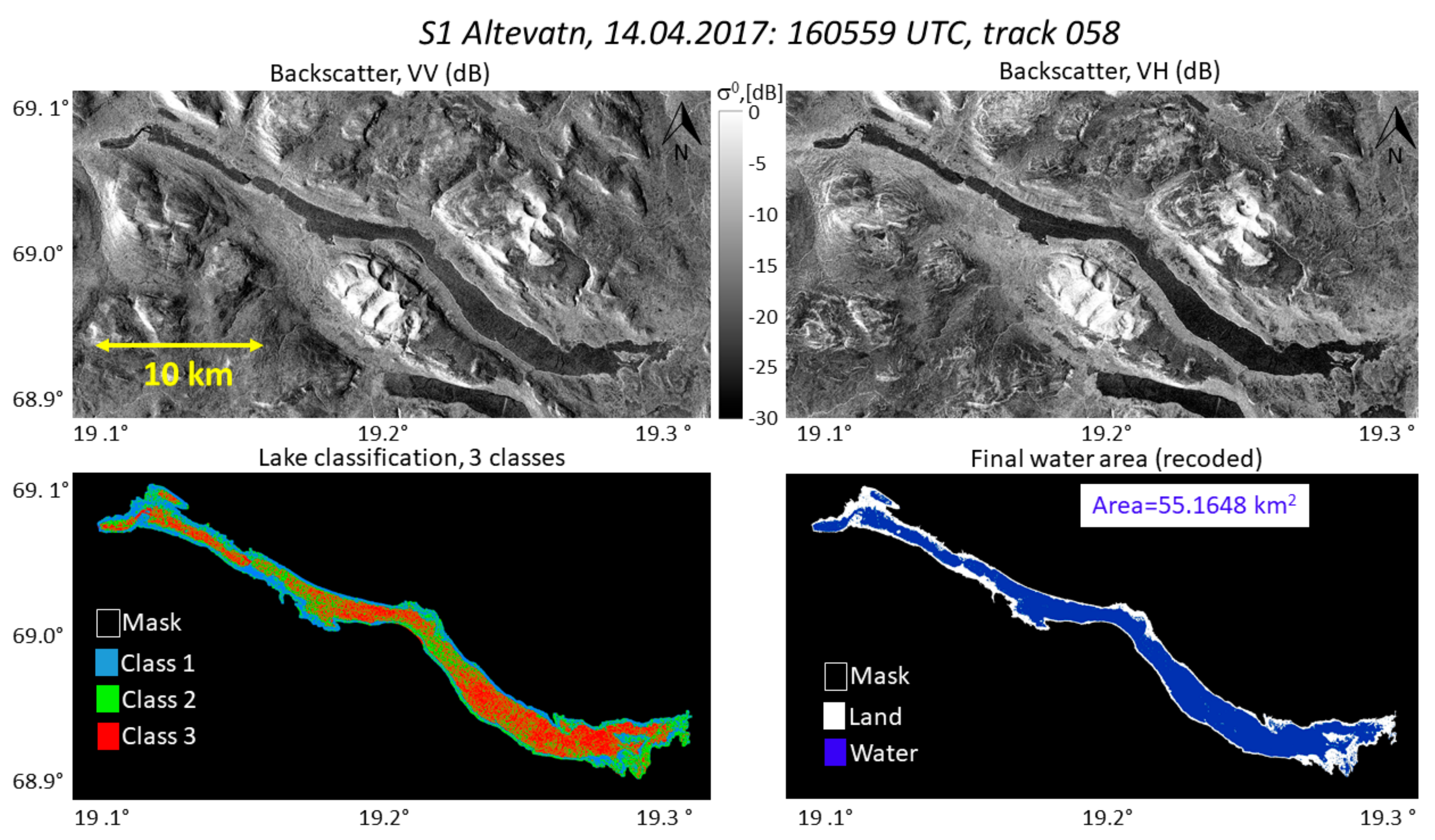
It is obvious there will be methods that are better suited to specific applications and case studies when compared with others that are more generic in nature, and similar to Gao et al. [7] we investigate in this study the suitability of K-means unsupervised clustering as a method to detect the water extent in SAR images for a typical arctic lake. We have chosen to implement this method over the more widely used techniques that involve fixed thresholds due to the high variability in backscatter for surface water that occurs due to waves and/or snow and ice cover. The K-means method works by separating the data samples into a specified number of clusters of equal variance by minimizing the sum of the square difference between the data samples and cluster mean, thereby finding the best class thresholds suited to a given image. The adaptive nature of the algorithm will in general be superior to hard threshold methods and has the advantage that it requires no manual intervention and is not dependent on training data, thereby making it a suitable generic analysis method compared to supervised methods that are trained on images with specific environmental conditions.

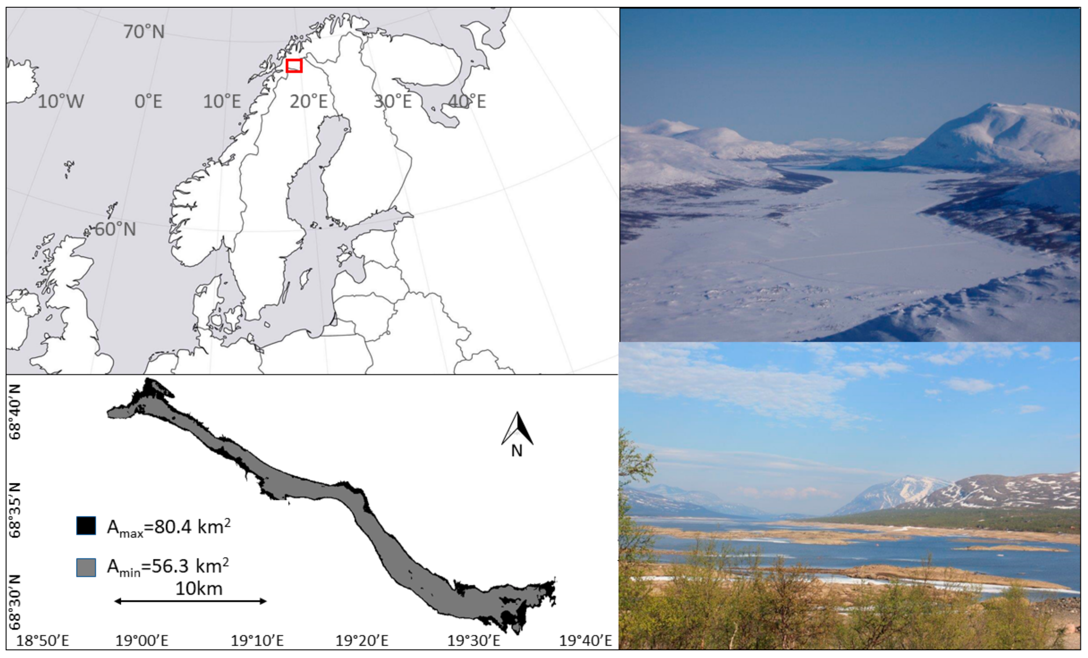
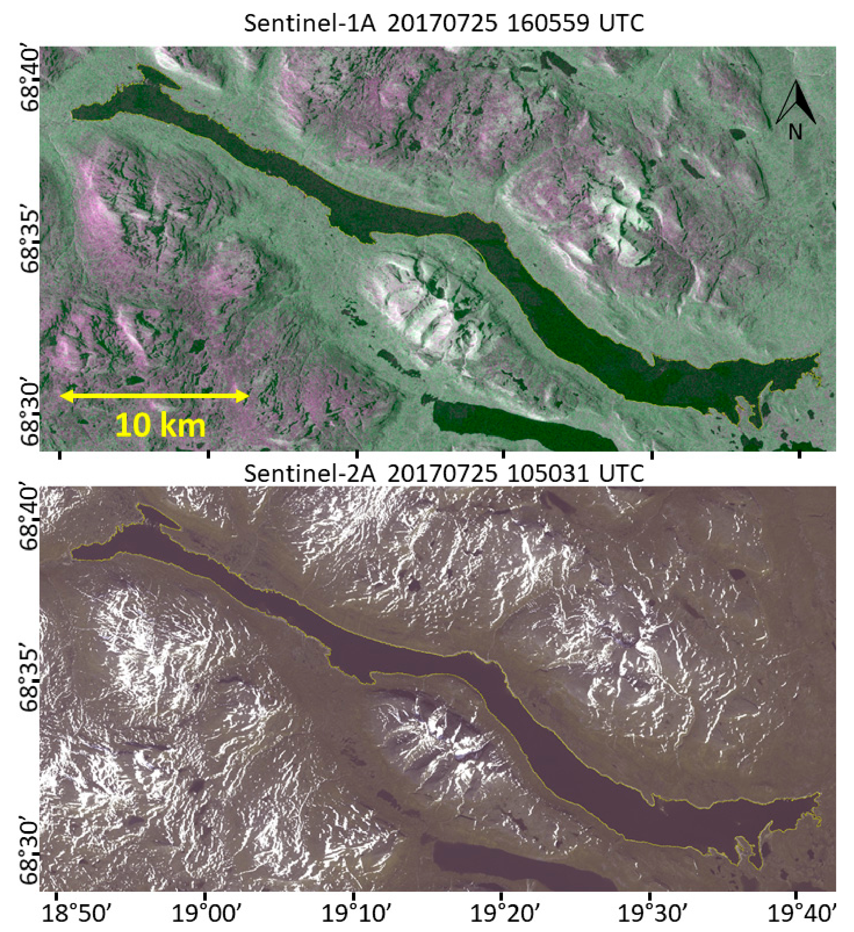
Altevatn (68.6N, 19.4E) is a medium-sized (79.71 km²) hydropower reservoir located in Bardu municipality in Northern Norway and is the 11th largest lake in Norway, with a maximum length and width of approximately 45 km and 2.5 km, respectively. It is bordered by mountainous terrain to the north and south and its water level exhibits an annual variation between 473 meters above sea level (m.a.s.l0 and 489 m.a.s.l, typically lowest before snowmelt commences in May and highest after most of the snow has melted (August/September). This results in a significant increase in the surface area (57–78 km²). 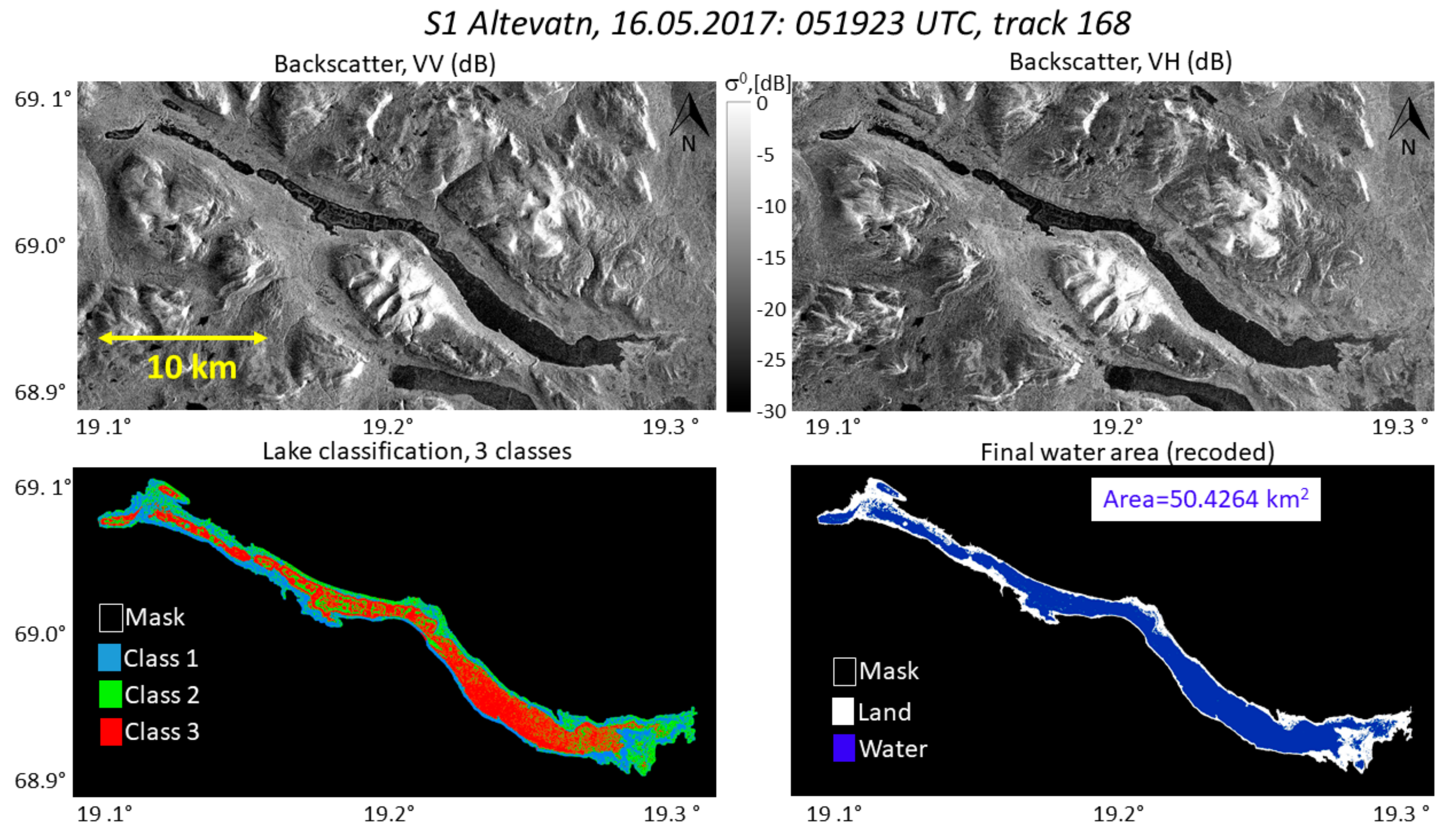Figure 1 illustrates the geographic location of Altevatn and its surrounding terrain. Water stored in the lake is regulated by a dam at its northwestern end and discharges into the river Bardu, and eventually empties into Malangen fjord via Målselva (river). While Altevatn is a medium-sized lake in a global context, it is quite large as a Scandinavian hydropower reservoir. Due to the accurate in-situ measurements and dense time series of Earth Observation (EO) data we find this dataset well suited to demonstrate how long-term monitoring of LWE in medium-sized lakes may be facilitated.

SAR backscatter from arctic lakes exhibits an annual variation as a result of seasonal snow and ice cover, which can build up from late autumn and last until the end of spring. During the summer and autumn when the lake is not frozen, the main challenge in estimating LWE is the variability in backscatter caused by surface roughness due to wind-induced waves at the water surface. This is a known problem particularly in co-polarized images which are most sensitive to surface roughness. In the freeze-up period, which typically takes place from November to January, the lake surface ice can be partial for a long period and presents a challenge when distinguishing water and land, since SAR backscatter from ice can exhibit very similar intensities to that from the surrounding land.

An additional complicating factor for monitoring Altevatn with SAR during the winter season is when the lake becomes entirely frozen with additional snow cover, which can result in greater radar backscatter than from open water, but lower backscatter than from bare ice, with the snow condition and depth affecting the strength of the backscatter. During the spring snowmelt or wet snow events during the winter, it becomes challenging to distinguish the lake edge since SAR backscatter from wet snow on land and lake can both be very low, thus giving poor contrast between the surface types. There is therefore a much greater degree of variability in backscatter during the winter and early spring, which results from varying ice and snow cover as well as snow condition, which is also controlled by temperature and precipitation. However, few studies have attempted to retrieve estimates of LWE during this challenging season and interpretation of SAR images will thus require a greater degree of care in order to extract the desired information. We intend to include where possible as many estimates of LWE from the winter season as we can, based on manual selection of the K-means classified images.

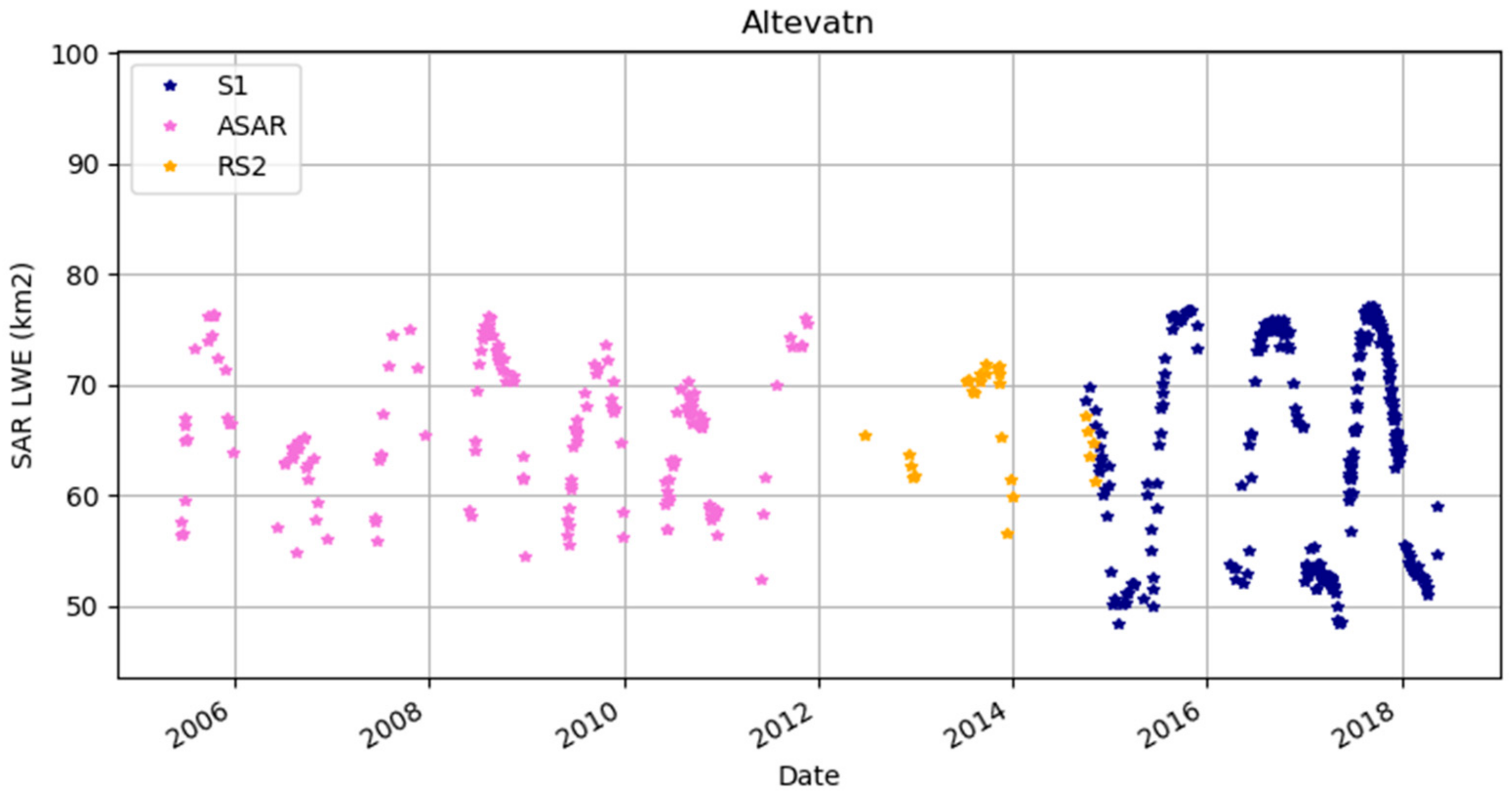
The primary objective of this study is to use C-band SAR images to estimate LWE for the Altevatn reservoir using three different SAR sensors, which together cover a period of almost 15 years. By employing as large a dataset as possible, in terms of number of images and period of time covered, we can check for consistency of the method over many seasons of data and across a range of sensor resolutions. We aim to develop a processing chain that not only will allow us to estimate and monitor the LWE of a single arctic lake but will be generic enough that it could be applied to any lake that is imaged by SAR satellites. We endeavor to achieve this by applying unsupervised clustering methods in order to firstly segment the SAR backscatter images and detect water occurrence in the SAR images.

The secondary objective is to use the LWE estimates to derive the lake hypsometry. That is to say, the relation between LWL and LWE through the use of in-situ water gauge measurements, and to apply this relationship to the measurement dataset to obtain not only a final time series of LWL but at the same time estimate the error in the LWE and LWL estimates. It is envisaged that this study will demonstrate an efficient and relatively simple method for monitoring variations in LWE (and therefore LWL) in near real-time. A similar study has earlier been carried out for monitoring water reservoir volume but in this case using optical Landsat imagery in combination with altimetry [22]. The capability to monitor water levels using only remote sensing data could be potentially valuable in situations where in-situ data may not be immediately available or in cases where shallow lakes undergo frequent and rapid changes in lake volume in response to changes in weather pattern, extreme droughts or human interaction (e.g., agriculture/irrigation). In the case of hydropower dams like Altevatn, the method may also have commercial applications since timely information on LWE/LWL can be interesting for power brokers to assess the future market.

2. Materials and Methods

2.1. SAR Datasets

SAR has been available since the launch of the European Space Agency (ESA) SAR satellite ERS-1 in 1991. However, time series of SAR images from this sensor are scarce. Since the launch of Envisat with the on-board advanced synthetic aperture radar (ASAR) sensor in 2002, the availability of SAR data has become more frequent. We have used ASAR wide swath data available as a dense time series since 2005. The data has 75 m pixel spacing and consists of scenes in both VV and HH (horizontally transmitted, horizontally received) polarization. We typically had coverage 6.8 times per month from 2005–2012 when we used all satellite geometries that cover the lake entirely. Envisat ASAR ceased to operate in April 2012.

Through the Norwegian RADARSAT-2 agreement we were able to continue the time series from 2012 to 2014 using the RS2 ScanSAR Narrow A mode with 25 m pixel spacing. This mode was delivered as single polarization VV scenes, but a majority of the data also had dual-polarization VV and VH scenes available. After the autumn of 2014 we chose to only use Sentinel-1 data as the main data source since this data set has both higher spatial and temporal resolution.

Sentinel-1 comprises two polar-orbiting satellites, Sentinel-1A, which was launched in April 2014 and Sentinel-1B, which was launched in April 2016. Sentinel-1 is a C-band SAR imaging mission whose interferometric wide swath mode (IW) covers a swath of approximately 250 km and is extended often up to 1000 km. The swath length varies according to a fixed observation pattern that is set by European Space Agency (ESA)/Copernicus as part of the operational monitoring program. The repeat time for identical image geometry is currently 12 days for each satellite and using data from both satellites the repeat pass time is therefore reduced to 6 days. Since the satellites have a polar orbit, high-latitude areas can be observed more frequently (every 2 to 3 days) at multiple viewing geometries. We used the S1 IW ground-range detected (GRD) product with pixel spacing of 10 m and utilized both polarization channels (VV/VH).

We acquired images from all imaging geometries that cover the Altevatn reservoir, though due to incomplete coverage of the entire lake, a proportion of the image dataset could not be used. For Sentinel-1, there were 5 geometries that completely covered Altevatn within a 6-day repeat cycle (track numbers 058, 095, 130, 160, and 168), which included 3 ascending and 2 descending passes. In addition, track 22 (descending) also covered Altevatn but only to a very small degree and was thus not used for calculating LWE. Track 66 covered the majority of the lake except for a small area at the easternmost end, however these images were used in the analysis by applying a correction for the missing data, which is described in greater detail in Section 3. For the Envisat ASAR dataset, 391 images with HH polarization were obtained from 49 different tracks that covered Altevatn over a timescale of 10 years. For RADARSAT-2, 112 images were obtained from 14 different geometries. For all sensors we used the ground-range detected (GRD) product, which delivered intensity images on a regular sampled grid. The multi-look factor, equivalent number of looks (ENL) for the sensors varied slightly.

Table 1. Sensors and sensor specifications used in the study. Number of scenes per sensor, and the number of scenes used for lake water extent (LWE) estimation after classification and post-filtering. ASAR: advanced synthetic aperture radar; ENL: equivalent number of looks.

Sensor	Time Period	Pixel Spacing	ENL (#looks)	Scenes	Used Scenes
Envisat ASAR	2005–2012	75 m	11.5	391	164
RADARSAT-2	2012–2014	25 m	4	112	26
Sentinel-1 A/B	2014–2018	10 m	4.4	786	295

summarizes the data availability and resolutions for each sensor used in this study. It should be noted that we were not able to use all SAR images in the dataset due to factors such as snow/ice cover and wind which resulted in poor contrast between the lake and surrounding land and resulting inaccurate classifications. These cases were visually identified and kept separate from the remainder of the dataset.

2.2. In Situ Water Level Gauge (Norwegian Water and Hydrology Directorate (NVE)/Statkraft)

Water levels were measured frequently in Altevatn using state of the art Digiquartz pressure gauges at the water intake for the hydropower pipe. The levels were logged hourly and the time series were smoothed with a Gaussian filter, with the smoothed value at midnight reported to the Norwegian Water and Hydrology Directorate in Norway (NVE) as the altitude of the lake surface above sea level. The sensor measurement accuracy was <1 cm. However, it is known that errors can occur due to sloping water levels during periods of wind buildup or periods with large pressure gradients over the lake. We requested the data set for the period 2002–2018 with daily average water level measurements. The water levels varied between 473 to 489 m.a.s.l depending on the seasonal changes (precipitation/snow melt) and the activity in the hydropower plant. The in-situ water level data were utilized in the final part of the processing scheme in order to derive regression coefficients that describe the relationship (hypsometry) between the estimated LWE from the SAR dataset and the observed water level. By deriving this relationship using over a decade of measurements we will be able to accurately predict the water level directly from future LWE estimates from SAR imaging. We also made use of the water levels to validate our results.

2.3. Data Processing and Methods

Prior to using and analyzing the SAR images, we first performed a precision SAR geocoding on all SAR images using the generic synthetic aperture radar (GSAR) software [23]. Here we used the calibrated Sentinel-1 IW ground range detected high resolution (GRDH) product, which was sampled with 10 m pixel spacing on the ellipsoid. The following geocoding steps were:

• Calibration using an annotated lookup table (from the GRDH product);
• Multi-looking, 2 × 2 pixels averaging to suppress speckle;
• Mapping the selected Universal Transverse Mercator (UTM)-projected output grid to the radar coordinates using a 10 m digital elevation model produced by the Norwegian Mapping Authority [24] and precision orbit vectors available from the European Space Agency (ESA) [25]
• Projection of the backscatter product to the output grid using the radar coordinate mapping (from step 3) and cubic interpolation.

The output radar backscatter images had units dB (σ⁰, VV, and VH) and were stored as a GeoTIFF using the UTM zone 33N, WGS-84 projection. The geocoding process also generated mask files for radar shadow and layover caused by the radar geometry and the terrain. Only small portions of the lake (<0.1%) are affected by layover/shadow and by using all available imaging geometries we are able to remove this problem entirely in the multi-temporal post-processing.

Once all images have been geocoded, the main part of the data processing chain that has been developed to derive LWE estimates is implemented. A pictorial overview of this processing chain, showing all steps from geocoded images to final LWE time series, is shown in Figure 2.

First, we applied a maximum area water mask to the input geocoded SAR images in order to reduce the image area to be segmented and thereby reduce computational time. To ensure that enough water and non-water pixels were contained within the lake mask, a morphological dilation filter was applied to the mask to increase the proportion of surrounding land area that was included in the classification. Once masking was implemented, we applied K-means clustering using 3 classes to segment the unmasked part of the image. Since we endeavored to include images from all seasons, it was assumed that the 3 classes represented backscatter from water, land, and ice; however, only the lowest class, representing detection low backscatter from water was used in the calculation of LWE. For images obtained between January and May inclusively, we used only cross polarization (VH) images from Sentinel-1 as inputs to the processing chain in order to make estimates of LWE during winter months. This was because the cross-polarization channel was much less affected by wind that often leads to increased backscatter in the VV channel and was therefore better suited to distinguishing ice cover that can often have similar backscatter amplitudes to wind-affected open water in the VV channel [9].

Once the entire dataset was segmented, the next step was post-processing and correcting the segmented images. First, pixels that were left unclassified due to being in areas of radar shadow/layover or due to incomplete coverage were corrected for using a multi-temporal method. This correction was made by selecting the nearest preceding image in the time series that had a different viewing geometry. We used the pixel classes from this image to classify the masked/unclassified pixels in the current image due to radar shadow/layover or missing data.

Next, a minimum area mask was applied to each image. This was necessary to correct for potential misclassifications due to wind or snow/ice at the lake surface. By correcting for these effects, we made use of a greater proportion of the dataset instead of discarding poor classifications. We constructed the minimum area mask by manually selecting images from June, since it was during this month that LWE for Altevatn reached its minimum extent during the snow-free season when there were good quality images with high contrast between land and water. The selection step was performed by inspecting the classified images against the original VV and VH images to ensure that only good classifications were used in constructing the minimum area mask and excluding those where effects of wind resulted in incorrect classifications. The minimum area mask was determined by mapping all pixels which had been classified as water and retaining only those pixels where water was always present in all June images; thus as our database of segmented images expanded with time. This minimum mask can be continually updated to take into account the fact that the minimum area in June during one season may not be representative for all years.

This will to a certain extent, correct misclassified pixels occurring within the center of the lake due to wind or other factors that may increase surface roughness and/or backscatter. The minimum area mask was however utilized differently for summer and winter images; for summer images, all pixels contained within the minimum area mask were classified as water (class 1) regardless of their original class. For winter classifications where pixels were often classified into class 1 or class 2 due to mixed backscatter, we reset all class 2 pixels to class 1 if they are contained within the minimum area mask; if there were class 2 pixels outside of this mask it is assumed they belong to the land class. The main difference between the treatment of summer and winter images is that pixels with class 3 occurring within the minimum area mask will always remain as class 3 in winter images, whereas in summer images they will always be reclassified to 1. After these corrections were made, a final detected water mask was constructed by choosing only the lowest class and this was median filtered to remove any remaining areas of speckle. We used this final water mask to calculate the LWE in km², using the known pixel size and total number of pixels in the water class. Figure 3 illustrates an example of the final lake classification from 25th July 2017, drawn as a vector outline on an RGB (red, green, blue composite) image of Altevatn, which was constructed using the VV image in the red and blue channels, and VH image in the green channel. We also acquired a cloud-free Sentinel-2 (S2) optical image from the same day and this was also shown in Figure 3 for comparison. In this example, the final lake classification corresponded to an outline that qualitatively agreed well with the edge of the lake deduced from the SAR RGB image as well as the Sentinel-2 image. There were a few places along the edge where the lake outline deviated with respect to the S2 image, but we considered this to constitute only a very small fraction (<1%) of the overall area. We intended to carry out a thorough quantitative comparison of S1 and S2 classification accuracy in a follow-up paper since it is not the goal of this study.

3. Results

In this section we present the time series of the LWE estimates obtained from implementing the data processing method described in Section 3. We further outlined how this is used to (a) derive the relation between the lake surface area and in-situ water level and (b) infer the water level for each satellite acquisition. Due to inaccuracies in estimating the surface area we also post-filtered the dataset to eliminate anomalous estimates and subsequently presented these best estimates as a time series.

3.1. Water Surface Area

In Figure 4 the complete time series of LWE estimates are shown for all satellite scenes that were classified using images from the three different sensors. This dataset is subsequently used as an input to the polynomial fitting to determine the lake hypsometry. Different colors were used to distinguish estimates made from Envisat ASAR (pink), RADARSAT-2 (orange), and Sentinel-1 (dark blue) images.

Figure 4 shows that LWE estimates typically vary between 49 km² and 78 km², with some years exhibiting greater maximum LWE than in other years. Since we only included estimates from winter months using the Sentinel-1 dataset it was not possible to ascertain whether the minimum estimated water levels were different between the three datasets. In terms of measurement density, there were 164 estimates made using Envisat ASAR data and 295 estimates from the Sentinel-1 datasets, which included some coverage during the winter months. The main difference was that the ASAR data span seven seasons while the Sentinel-1 data in this time series span only four full seasons, indicating that not only does Sentinel-1 have a higher spatial resolution but also far more superior temporal resolution in LWE than the ASAR dataset. The annual cycle of LWE increasing and decreasing was apparent throughout the time series and due to regulation of water volume by the dam in addition to the influence of meteorological factors affecting the maximum annual water level.

3.2. Regression between LWE and LWL (Hypsometry)

In a closed lake system, a unique relationship exists between LWE and LWL. For Altevatn where daily in-situ water level measurements are available, we fitted a polynomial function to the final LWE time series to derive coefficients that describe the relationship between SAR LWE estimates and measured lake water level (LWL) as provided by NVE. The majority of the dataset comprises images from the snow-free season when the lake was not close to its minimum water level and a linear relationship between LWE and LWL was expected. However, since we included LWE estimates made during the winter/spring season when snow and/or ice was present, it cannot be expected that LWE inferred from the SAR images will vary linearly with LWL due to the different densities of water and snow/ice. Therefore, we investigated the applicability of fitting a natural spline and first-, second-, and third-order polynomials to the dataset. Ultimately, we wish to acquire a function that describes the relationship between the LWE estimated from SAR and the actual LWL measurement with as small an error as possible. This could therefore be utilized in a near real-time context so that LWL can be estimated directly from LWE estimates made from incoming SAR images. By calculating the root mean squared error (RMSE) of the different fits, we will be able to assess which function gives the most appropriate and accurate description of the lake hypsometry.

The first stage of deriving the lake hypsometry involves making an initial fit to the entire dataset with the spline/polynomial function, then using the fit coefficients to compute the corresponding time series of LWE using the in-situ LWL dataset. This “model” time series of LWE was used to filter the SAR dataset by removing data points where the error (difference) between the SAR and NVE in-situ data estimates of LWE exceeded 7.5% of the maximum area variation as exhibited by the NVE LWE time series. We investigated two cases for the initial filtering of the SAR LWE dataset; firstly when the third-order polynomial fit was used to obtain estimates of LWE from the in-situ LWL and secondly, when the natural spline fit was used to obtain LWE from LWL. Filtering the original LWE dataset using the two different functions resulted in a slightly different number of datapoints removed, since the errors in the retrieved LWE estimate (from in-situ LWL) were different, while the threshold was the same. Using the third-order polynomial, 332 data points remained in the filtered dataset while the natural spline fit resulted in 376 data points remaining.

By removing outliers from the original dataset, we were able to refine the linear, polynomial, and spline fits and obtain a new set of coefficients with which to apply to the original dataset. These improved fits using linear, polynomial or natural spline functions, are shown in Figure 5.

It can be seen from Figure 5 that the inclusion of LWE estimates from the winter months are associated with the lowest measured water levels and that the inclusion of these data tens to shift the relationship between LWE and LWL from linear to nonlinear. The RMSE for both second- and third-order polynomials was respectively 0.904 km² and 0.892 km², indicating that the fit of the third-order polynomial was roughly identical to using the second-order polynomial. The application of a natural spline reduced the RMSE only marginally to 0.882 km². For a mean lake area of approximately 65 km² this corresponds to an error of 1.4%. By comparison, the RMSE associated with applying a linear fit (1.14 km²) was equivalent to approximately 1.7% of the mean area.

For reference, we included an example of the classification of an image from 14 April 2017 in Figure 6. Here the original VV and VH backscatter images are shown in the upper two panels, while the original classification is shown in the lower left panel and the final classification, after correction using the minimum mask, is shown in the lower right panel. The color scheme for the original classification shows the lowest class (1) in blue, class 2 pixels in green, and class 3 pixels in yellow. For a typical summer image, the lake should comprise only blue colored pixels and land may consist of either class 2 or class 3 pixels, depending on the backscatter intensity. In this example however we see that there are many mixed class 1 and class 2 within the lake area, but using the current scheme of using the minimum area mask to correct the class 2 pixels that are contained within the minimum area, we obtained a final classification that resulted in an estimated LWE of 55.16 km² with an error of only 0.26 km² (0.48%), suggesting that the LWE estimate inferred from this final classification of the water covered area was very accurate, despite that there were still some misclassified pixels remaining within the water covered area.

On the other hand, we also show in Figure 7 an example of an image, which was excluded after filtering the dataset due to the error in the estimated SAR LWE exceeding the threshold. In this example from 16 May 2017, the error in the estimated LWE was −2.68 km² while the in-situ LWL was at a low level of 474.52 m. This indicates that the SAR estimate was too low with respect to the LWE estimated using the polynomial fit coefficients and the NVE LWL measurement on this date. Qualitatively, the final classification appears to contain too many water pixels with respect to the low (dark) backscatter in the VH image, rather than too few. This may suggest that anomalous data points in the dataset skewed the fitted polynomial such that the LWE estimated from the in-situ LWL measurements were too high, therefore leading to larger errors when the SAR LWE was low and more estimates were filtered out based on error estimates. It may therefore be necessary to pre-filter the dataset for strong outliers prior to fitting a polynomial function, such that the initial fit provides reliable coefficients and therefore a reliable threshold with which to reduce the dataset.

The refined fits, as shown in Figure 5, were used to calculate a new time series using the original (unfiltered) SAR LWE dataset, which was refiltered using the same constraints on the threshold criteria. This refiltered SAR LWE dataset was next used to obtain the inverse relation describing LWL as a function of SAR LWE. This was done by repeating the fitting to the in-situ LWL and applying the fit coefficients of the chosen function to the datapoints remaining in the SAR LWE time series. Figure 8 illustrates this regression step for the entire SAR dataset, where the winter month estimates are indicated by a turquoise color. In both cases of obtaining either the LWE–LWL relationship (Figure 5) or the LWL–LWE relationship (Figure 8), there is an improvement in the RMSE obtained by fitting a nonlinear function to the dataset, but with only minor reductions in the error from fitting a natural spline or second- and third-order polynomials. In addition, there was a small difference in RMSE obtained using the different functions, depending on which function was used to perform the initial filtering of the original dataset as noted earlier. This difference was likely due to the different numbers of datapoints remaining after filtering, with slightly higher RMSE resulting from more datapoints being kept, as in the case of filtering with the initial spline fit. We summarize these differences in

Table 2. RMSE associated with fitting linear, second- and third-order polynomials, and natural spline functions to in-situ LWL (obtaining LWE) and SAR LWE (obtaining LWL), using either the fitted third-order polynomial or natural spline function to perform the initial filtering of the original dataset.

	RMSE LWE, km2	RMSE LWL, m	RMSE LWE, km2	RMSE LWL, m
Initial Filtering	Order 3 polynomial		Spline
Linear	1.136	0.505	1.229	0.492
Second-Order Polynomial	0.904	0.437	1.106	0.443
Third-Order Polynomial	0.892	0.419	1.091	0.434
Natural Spline	0.882	0.403	1.082	0.421

.

Of course, by increasing or lowering the threshold which was used to filter the dataset, the number of datapoints remaining in the filtered dataset can also be increased or decreased respectively, thereby also changing the RMSE in the inferred LWE/LWL estimates. Nonetheless, we found that this threshold provided a satisfactory compromise between accuracy in the derived LWL and retaining a satisfactory temporal coverage in the final time series.

In Figure 9 we applied the third-order polynomial to the LWE estimates in the filtered SAR dataset. The resulting time series of LWL is shown in the upper panel of Figure 9, while the lower panel in Figure 9 shows the error in these LWL estimates, defined as the difference between LWL estimated with SAR and the corresponding in-situ LWL measurement. With the exception of the period 2012–2013, covered by the RADARSAT-2 operations, SAR LWE and LWL estimates cover all other years in the time series, with as expected very good coverage by Sentinel-1 from 2016 onwards when both Sentinel-1A and 1B satellites were in operation. Inspection of the errors, shown in the lower panel of Figure 9 shows that the largest uncertainties in the LWL estimates are not strictly associated with a particular time of year, though the smallest errors do tend to be tied to times when the lake water level is at its greatest, and increase either side of the maximum water level.

4. Discussion

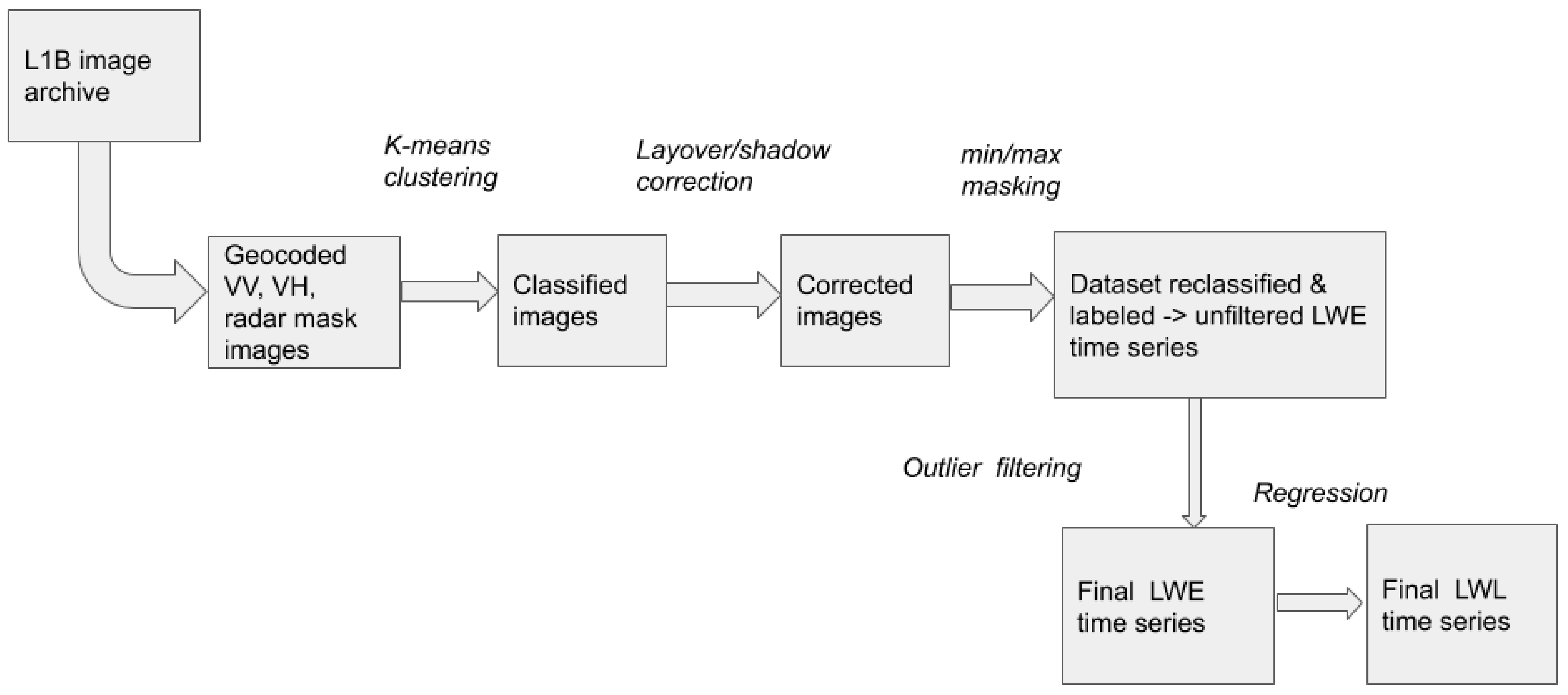
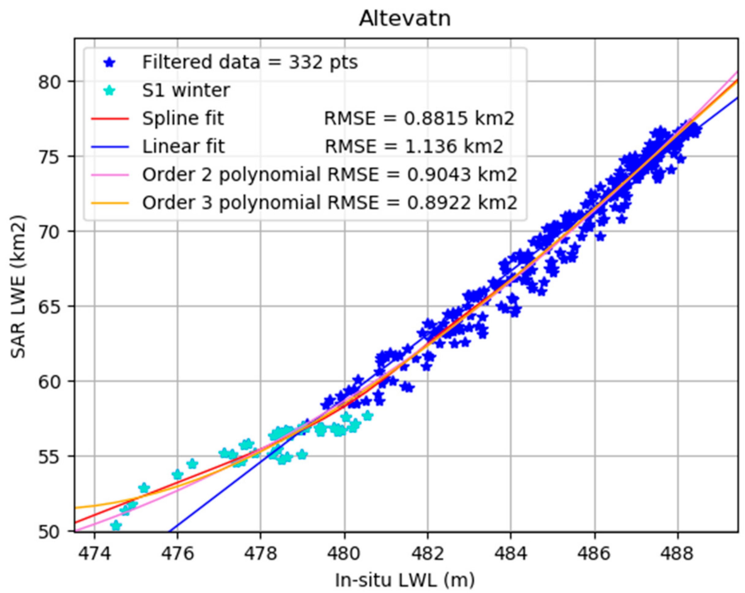
In this work we developed and demonstrated the use of a simple processing chain for estimating lake water extent using SAR images acquired by the Envisat ASAR, RADARSAT-2, and Sentinel-1 missions for the Altevatn reservoir in Northern Norway. Our method for estimating LWE is anchored in the use of unsupervised classification to detect surface water cover in the SAR images. Additionally, we have shown that by combining SAR estimates with in-situ measurements of LWL, the hypsometric curve for a lake can be obtained by fitting a third-order polynomial to describe the relationship between SAR LWE and LWL. In the present study we endeavored to show that estimates of LWE can be made during the winter months when challenges related to snow and ice cover may be present. On the other hand, the main challenge in correctly detecting lake water cover during the summer months is due to changes in surface roughness, usually resulting from the effect of wind over open water. We have however, included a correction in our processing chain to account for misclassifications within the center region of the lake that may arise due to the increased backscatter from waves, by applying a minimum area mask on each image.

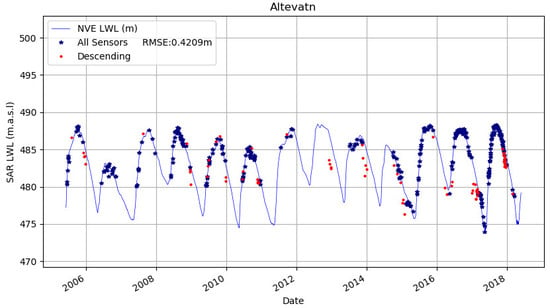
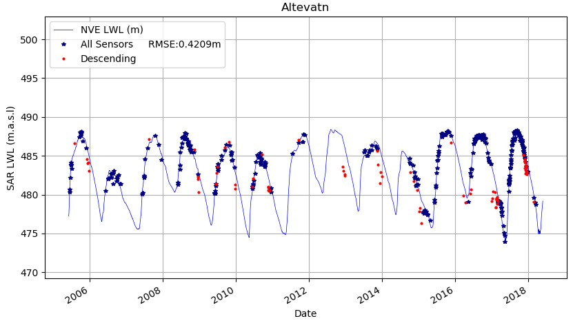
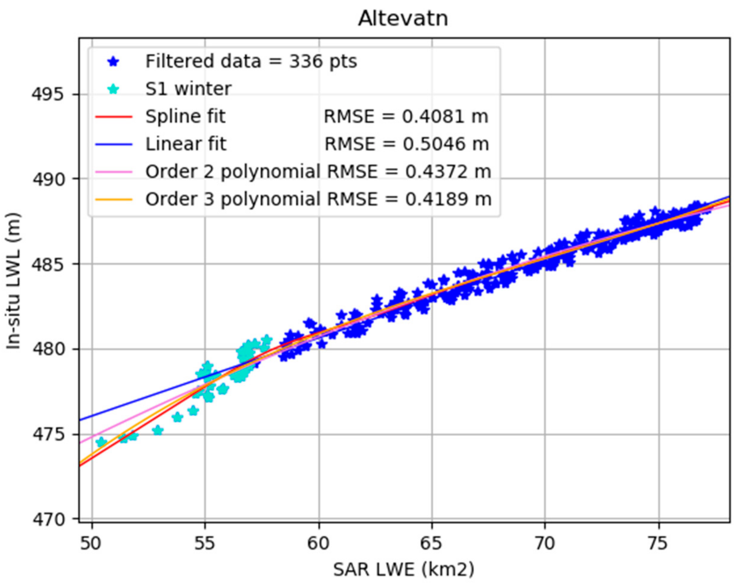
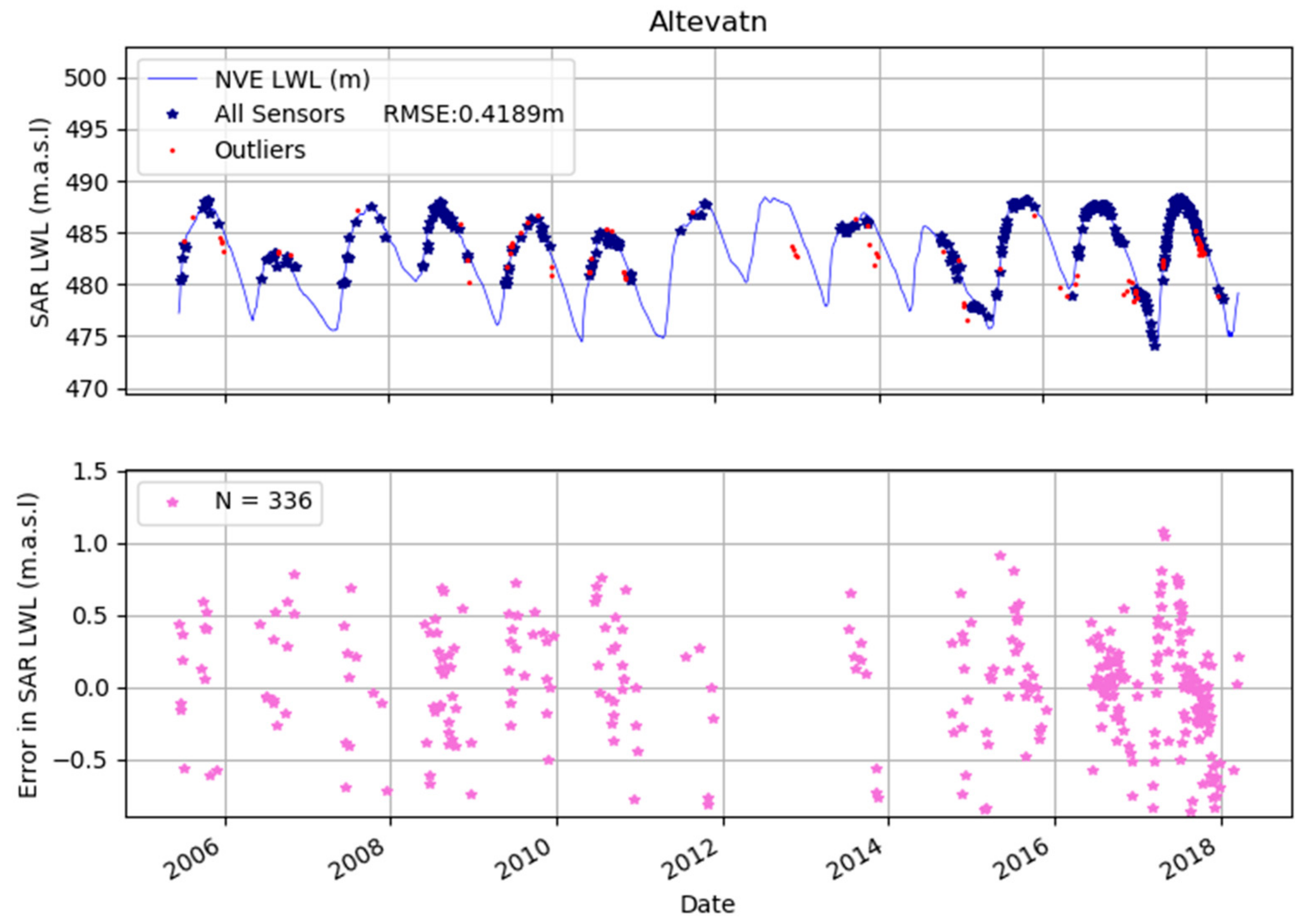
We have processed approximately 14 years of SAR data from sensors with different spatial resolutions and shown that even when using images with the lowest resolution of 75 m (Envisat ASAR) it is nevertheless possible to obtain a time series of LWE and derived LWL that is in qualitatively good agreement with the in-situ measurements. Through filtering and reducing the datasets we have been able to obtain fitted functions that allow LWL estimates to be made with the lowest RMS error obtained of 0.403 m, which is 2.5% of the maximum water level variation of the lake during the period studied. We found that only minor improvements in the RMSE were obtained from fitting a natural spline function compared with second- and third-order polynomials. Using the present threshold for filtering the dataset resulted in only 73 estimates of LWL that met the GCOS accuracy requirement of 10 cm for medium-sized lakes, which was roughly 21% of the filtered dataset. These estimates were associated with the months ranging from March through to December, indicating that there was no preference for better accuracy during the snow-free months. Furthermore, it is both interesting and important to note that estimates made with the lowest resolution sensor (ASAR) do not exhibit noticeably greater errors in the derived LWL estimates compared with the errors associated with the RS2 and Sentinel-1 estimates which both have much higher spatial resolution.

We obtained the lake hypsometry by fitting linear and nonlinear functions to the LWE–LWL datasets, with improvements in the RMSE of LWE and LWL when a natural spline or higher order polynomials were applied. We observed a mostly linear relationship for data samples associated with the summer (snow and ice free) months whereas the nonlinearities in the relationship were introduced as a result of including estimates made during the winter/spring months. This is likely due to the fact that the in-situ LWL is inferred from pressure gauge measurements and thus does not take into account the density differences of ice, snow, and water but instead indicates the water level equivalent for a given pressure. Since snow and ice are less dense than water, then the total ice/water covered area for a given equivalent water content will be greater than if the area had been derived from only water cover. This explains the observed relationships depicted by the scatter plots of Figure 5 and Figure 8.

The smallest LWE and LWL are typically associated with the end of the winter months and during the transition period when wet snow or ice present on land can present a challenge since this appears as low backscatter in the SAR images and gives little contrast between land and water. There may therefore be gaps in the coverage of the lowest LWL and LWE estimates due to poorer conditions for making reliable classifications. In such cases the problem could be addressed by taking into account the temporal history of the land/water classifications and allowing the minimum and maximum area masks to be dynamic, thereby limiting the uncertainty and variability of the LWE during transitional periods. Additionally, the use of wet snow maps for identifying areas of uncertainty would assist in developing a more automated detection of erroneous classifications. For example, if pixels associated with wet snow cover are found to intersect the area contained within the lake mask, then it could be expected that the classified area of water would be overestimated if only the backscatter amplitudes were used to classify the image. Adding wet snow maps as an input feature, as well as backscatter amplitudes to the K-means classifier could for example assist in identifying small differences in backscatter between wet snow on land and open water. Including additional information such as digital elevation map (DEM), slope, and land cover maps in training maximum likelihood classifiers for flood mapping applications has also been shown to reduce misclassifications due to the effects of noise and topography [26].

Even though the current methodology is not yet fully automated, we see a potential to develop the procedure such that the current processing chain could be used in an operative, real-time setting. For this to be possible, the final lake classifications would have to be automatically checked for poor quality or by some other measure to indicate the quality of the original image being used in the classification. For example, by identifying VV images that are affected by wind and therefore higher backscatter across the surface, selecting only the VH channel to be used for classification could be implemented, possibly resulting in fewer poor classifications that are discarded from the final LWE time series. The LWE estimate derived from the final classified image could also be quality controlled by comparing it against some moving average of the earlier data points to determine whether or not it falls into the expected level of variation based on previous values. Automatic quality checks such as those suggested here would be required in order to bring the current procedure up to the standard demanded of a real time processing system.

One of the objectives for this study was to develop a processing chain that could be generic enough to be applied to any other lake; in the current processing chain we have studied a relatively small lake where incidence angle is unlikely to cause significant variation in backscatter across the lake. However, for very large lakes, it would be necessary to make corrections for local incidence angle variations in the SAR image since this affects backscatter strength [27] at near and far ranges. The effect of incidence angle on backscatter is also dependent on the structural and dielectric properties of the surface [28], which can be different, for example, in water bodies that are highly turbid or vegetated. This would have to be accounted for if our method was to be applied to such cases. Indeed, some of the common challenges resulting in misclassification, such as wind-induced increase in backscatter at the lake surface, may be addressed by using the incidence-angle dependence of different surfaces as O’ Grady et al. [29] have demonstrated. On the other hand, another approach to dealing with backscatter variations due to incidence angle variations may be to divide up the image into segments or bands of roughly constant incident angles, as previous authors have investigated [30].

A final topic that may have to be addressed if the method were to be transferrable to any other lake globally is the concept of the minimum area mask. We demonstrated in this study how we can obtain and apply such a product in order to correct for misclassifications and thereby retain a greater number of images in the time series. In the case of Altevatn this was made possible by the fact that the lake water volume is regulated and reaches a minimum at a certain time of year. This information may not be available for the majority part of unregulated lakes, which would therefore present a challenge in knowing which images to use to put together such a mask. Additionally, there are many shallow lakes in regions of the world where the lake dries up completely and the concept of a minimum water area would thus be irrelevant. It may therefore be necessary to adjust the current method in such a way that a minimum area mask becomes only an optional component of the processing rather than a mandatory one. For example, instead of segmenting the image into only three classes it could be worth investigating the use of over-segmentation and using more classes to separate areas of water with different backscatter characteristics. These could for example be combined as part of the post-processing to represent the final water covered area. At present our method is not good enough to obtain LWL at the level of precision demanded by GCOS while retaining satisfactory temporal coverage. In order to achieve the GCOS-requirement for the LWL (10 cm accuracy) we would need to improve the single pass classification accuracy close to 100%. Considering the challenges due to variable conditions including ice and wind this is unlikely with current SAR sensors. There is, however, a potential in the multi-temporal filtering of individual pixel classifications that could improve the accuracy significantly. A similar approach was used for snow monitoring [31] and opens the possibility for fusing multiple sensors such as S1 and S2. This task will be studied in future work.

5. Conclusions

We have shown that a consistent time series of the lake water extent (LWE) can be derived from SAR data on a decadal scale for a medium-sized arctic lake using a variety of historical sensors and taking care of biases caused by variable sensor capabilities. Our methods are based on K-means classification of radar backscatter and careful post-processing to omit ill-posed scenes due to particularly challenging lake conditions.

By relating the LWE estimates to in-situ lake water level (LWL) measurements we have demonstrated that the lake hypsometry (the functional relationship between LWE and LWL) may be inferred and using this we derived the corresponding LWL by measuring LWE from SAR. We are also able to assess the RMSE errors for each individual LWE estimate, seasonal fluctuations in RMSE, and biases mainly caused by the spatial resolution of the various sensors. The accuracy depends highly on the sensor in use but Sentinel-1 has of the order 1.4% accuracy, which is far better than the desired accuracy of GCOS (10%). The derived LWL on the other hand, has an accuracy of 40 cm vs. the GCOS requirement of 10 cm for medium-sized lakes. This reciprocal relationship in accuracy between LWE and LWL shows that the hypsometric method has some weaknesses that need to be addressed in order to improve the accuracy of the derived LWL.

Our study has made use of three different SAR sensors, each dataset covering almost independent periods of the 13-year time series. Despite that the three sensors ranged in resolution from 10 m to 75 m, our results did not reveal any distinct sensor bias in the overall LWE error estimates.

Future work will adapt the methods above on lakes on a global scale in the ESA project CCI (Climate Change Initiative) Lakes. We also intend to investigate methods to automate the processing and handle winter conditions with ice cover and melting snow. We will also attempt to quantify classification errors better by comparing close to simultaneous Sentinel-1 and Sentinel-2 images.

References

1. Crétaux, J.F.; Jelinski, W.; Calmant, S.; Kouraev, A.; Vuglinski, V.; Bergé-Nguyen, M.; Maisongrande, P. SOLS: A lake database to monitor in the Near Real Time water level and storage variations from remote sensing data. Adv. Space Res. 2011, 47, 1497–1507. [Google Scholar] [CrossRef]
2. Frappart, F.; Biancamaria, S.; Normandin, C.; Blarel, F.; Bourrel, L.; Aumont, M.; Azemar, P.; Vu, P.-L.; Le Toan, T.; Lubac, B.; et al. Influence of recent climatic events on the surface water storage of the Tonle Sap Lake. Sci. Total Environ. 2018, 636, 1520–1533. [Google Scholar] [CrossRef] [PubMed]
3. Xing, L.; Tang, X.; Wang, H.; Fan, W.; Wang, G. Monitoring monthly surface water dynamics of Dongting Lake using Sentinel-1 data at 10 m. Peer Rev. J. 2018, 6, e4992. [Google Scholar] [CrossRef] [PubMed]
4. Miles, K.E.; Willis, I.C.; Benedek, C.L.; Williamson, A.G.; Tedesco, M. Toward Monitoring Surface and Subsurface Lakes on the Greenland Ice Sheet Using Sentinel-1 SAR and Landsat-8 OLI Imagery. Front Earth Sci. 2017, 5, 58. [Google Scholar] [CrossRef]
5. Bolanos, S.; Stiff, D.; Brisco, B.; Pietroniro, A. Operational Surface Water Detection and Monitoring Using RADARSAT 2. Remote Sens. 2016, 8, 285. [Google Scholar] [CrossRef]
6. Bioresita, F.; Puissant, A.; Stumpf, A.; Malet, J. A Method for Automatic and Rapid Mapping of Water Surfaces from Sentinel-1 Imagery. Remote Sens. 2018, 10, 217. [Google Scholar] [CrossRef]
7. Gao, H.; Birkett, C.; Lettenmaier, D.P. Global monitoring of large reservoir storage from satellite remote sensing. Water Resour. Res. 2012, 48, W09504. [Google Scholar] [CrossRef]
8. Sobiech, J.; Dierking, W. Observing lake- and river-ice decay with SAR: Advantages and limitations of the unsupervised k-means classification approach. Ann. Glaciol. 2013, 54, 65–72. [Google Scholar] [CrossRef]
9. Wang, J.; Duguay, C.R.; Clausi, D.A.; Pinard, V.; Howell, S.E.L. Semi-Automated Classification of Lake Ice Cover Using Dual Polarization RADARSAT-2 Imagery. Remote Sens. 2018, 10, 1727. [Google Scholar] [CrossRef]
10. Yu, Q.; Clausi, D.A. IRGS: Image segmentation using edge penalties and region growing. IEEE Trans. Pattern Anal. Mach. Intell. 2008, 30, 2126–2139. [Google Scholar]
11. Bangira, T.; Alfieri, S.M.; Menenti, M.; van Niekerk, A. Comparing Thresholding with Machine Learning Classifiers for Mapping Complex Water. Remote Sens. 2019, 11, 1351. [Google Scholar] [CrossRef]
12. Zhou, Y.; Wang, H.; Xu, F.; Jin, Y.-Q. Polarimetric sar image classification using deep convolutional neural networks. IEEE Geosci. Remote Sens. Lett. 2016, 13, 1935–1939. [Google Scholar] [CrossRef]
13. Chen, S.; Wang, H.; Xu, F.; Jin, Y.-Q. Target classification using the deep convolutional networks for SAR images. IEEE Trans. Geosci. Remote Sens. 2016, 54, 4806–4817. [Google Scholar] [CrossRef]
14. Wang, L.; Scott, K.A.; Xu, L.; Clausi, D.A. Sea Ice Concentration Estimation during Melt from Dual-Pol SAR Scenes Using Deep Convolutional Neural Networks: A Case Study. IEEE Trans. Geosci. Remote Sens. 2016, 54, 4524–4533. [Google Scholar] [CrossRef]
15. Bianchi, F.M.; Grahn, J.; Eckerstorfer, M.; Malnes, E.; Vickers, H. Snow avalanche segmentation in SAR images with Fully Convolutional Neural Networks. IEEE Trans. Geosci. Remote Sens 2019. under review. [Google Scholar]
16. Acharya, T.D.; Subedi, A.; Lee, D.H. Evaluation of Machine Learning Algorithms for Surface Water Extraction in a Landsat 8 Scene of Nepal. Sensors 2019, 19, 2769. [Google Scholar] [CrossRef]
17. Isikdogan, F.; Bovik, A.C.; Passalacqua, P. Surface water mapping by deep learning. IEEE J. Sel. Top. Appl. Earth Obs. Remote Sens. 2017, 10, 4909–4918. [Google Scholar] [CrossRef]
18. Jiang, W.; He, G.; Long, T.; Ni, Y.; Liu, H.; Peng, Y.; Lv, K.; Wang, G. Multilayer Perceptron Neural Network for Surface Water Extraction in Landsat 8 OLI Satellite Images. Remote Sens. 2018, 10, 755. [Google Scholar] [CrossRef]
19. Xie, H.; Luo, X.; Xu, X.; Pan, H.Y.; Tong, X.H. Evaluation of Landsat 8 OLI imagery for unsupervised inland water extraction. Int. J. Remote Sens. 2016, 37, 1826–1844. [Google Scholar] [CrossRef]
20. Yu, L.; Wang, Z.; Tian, S.; Ye, F.; Ding, J.; Kong, J. Convolutional neural networks for water body extraction from Landsat imagery. Int. J. Comput. Intell. Appl. 2017, 16, 1750001. [Google Scholar] [CrossRef]
21. Pham-Duc, B.; Prigent, C.; Aires, F. Surface Water Monitoring within Cambodia and the Vietnamese Mekong Delta over a Year, with Sentinel-1 SAR Observations. Water 2017, 9, 366. [Google Scholar] [CrossRef]
22. Abileah, R.; Vignudelli, S.; Scozzari, A. A completely remote sensing approach to monitoring reservoirs water volume. Int. Water Technol. J. 2011, 1, 63–77. [Google Scholar]
23. Larsen, Y.; Engen, G.; Lauknes, T.R.; Malnes, E.; Høgda, K.A. A generic differential interferometric SAR processing system, with applications to land subsidence and snow-water equivalent retrieval. In Proceedings of the Fringe ATSR Workshop 2005, Frascati, Italy, 28 November–6 December 2005. [Google Scholar]
24. Norwegian Mapping Authority. Available online: https://kartverket.no (accessed on 21 October 2019).
25. Sentinel-1 Quality Control. Available online: https://qc.sentinel1.eo.esa.int (accessed on 21 October 2019).
26. Hong, S.; Jang, H.; Kim, N.; Sohn, H.-G. Water Area Extraction Using RADARSAT SAR Imagery Combined with Landsat Imagery and Terrain Information. Sensors 2015, 15, 6652–6667. [Google Scholar] [CrossRef] [PubMed]
27. O’Grady, D.; Leblanc, M.; Gillieson, D. Relationship of local incidence angle with satellite radar backscatter for different surface conditions. Int. J. Appl. Earth Observ. Geoinf. 2013, 24, 42–53. [Google Scholar] [CrossRef]
28. Ulaby, F.T.; Moore, R.K.; Fung, A.K. Radar Remote Sensing and Surface Scattering and Emission Theory, 2nd ed.; Addison-Wesley: New York, NY, USA, 1982. [Google Scholar]
29. O’Grady, D.; Leblanc, M.; Bass, A. The use of radar satellite data from multiple incidence angles improves surface water mapping. Remote Sens. Environ. 2014, 140, 652–664. [Google Scholar] [CrossRef]
30. Haarpaintner, J.; Solbø, S. Automatic Ice-Ocean Discrimination in SAR Imagery; Norut Northern Research Institute: Tromsø, Norway, 2007. [Google Scholar]
31. Solberg, R.; Amlien, J.; Koren, H.; Eikvil, L.; Malnes, E.; Storvold, R. Multi-sensor and time-series approaches for monitoring of snow parameters. IEEE Int. Geosci. Remote Sens. Symp. 2014, 3, 1661–1666. [Google Scholar]
Figure 1. Left (top): location of study area in Northern Scandinavia (red rectangle). Left (bottom): summer maximum and minimum water mask. Right (top): winter photo from Altevatn. Right (bottom): spring photo at low water level (photos: Kjell Arild Høgda).
Remotesensing 11 02780 g001
Figure 2. Processing chain for derivation of LWE and lake water level (LWL) time series.
Remotesensing 11 02780 g002
Figure 3. Top: Sentinel-1A RGB-composite (VV, VH, VV) over Altevatn from 25th July 2017. Bottom: Sentinel-2A RGB (Ch4, Ch3, Ch2) from 25 July 2017 over the same area. The S1 classified water edge vector was superimposed on both the S1 RGB and S2 image in a yellow color.
Remotesensing 11 02780 g003
Figure 4. Lake water extent in km2 per satellite acquisition.
Remotesensing 11 02780 g004
Figure 5. LWE–LWL regression step showing the final natural spline, polynomial, and linear fits made to the filtered data set. In this example the original data set was filtered using the initial polynomial fit. RMSE: root mean squared error.
Remotesensing 11 02780 g005
Figure 6. Example of the classified lake area from 14 April 2017 where the error in LWE was low.
Remotesensing 11 02780 g006
Figure 7. Example of the classified lake area from 16 May 2017 which was identified to be an outlier due to the error in LWE exceeding the defined threshold.
Remotesensing 11 02780 g007
Figure 8. Scatter plot of the Sentinel-1 LWE estimates vs. corresponding in-situ measurements of lake water level, shown together with fitted natural spline function, polynomials of first-, second-, and third-order, and the respective RMSE in the LWL estimates.
Remotesensing 11 02780 g008
Figure 9. Final LWL time series derived from applying the third-order polynomial to the filtered LWE dataset. Data points identified as outliers from the initial polynomial fit made to the LWE–LWL dataset are shown in red. These were not used further in fitting a polynomial to the LWL–LWE dataset. m.a.s.l: meters above sea level.
Remotesensing 11 02780 g009