Article

An Evaluation and Comparison of Four Dense Time Series Change Detection Methods Using Simulated Data

1
Department of Geography and Earth Sciences, Aberystwyth University, Aberystwyth SY23 3DB, UK
2
Environment Systems Ltd., 9 Cefn Llan Science Park, Aberystwyth SY23 3AH, UK
*
Author to whom correspondence should be addressed.
Remote Sens. 2019, 11(23), 2779; https://doi.org/10.3390/rs11232779
Submission received: 22 October 2019 / Revised: 19 November 2019 / Accepted: 22 November 2019 / Published: 25 November 2019
(This article belongs to the Section Remote Sensing in Agriculture and Vegetation)

Abstract

:
Access to temporally dense time series such as data from the Landsat and Sentinel-2 missions has lead to an increase in methods which aim to monitor land cover change on a per-acquisition rather than a yearly basis. Evaluating the accuracy and limitations of these methods can be difficult because validation data are limited and often rely on human interpretation. Simulated time series offer an objective method for evaluating and comparing between change detection algorithms. A set of simulated time series was used to evaluate four change detection methods: (1) Breaks for Additive and Seasonal Trend (BFAST); (2) BFAST Monitor; (3) Continuous Change Detection and Classification (CCDC); and (4) Exponentially Weighted Moving Average Change Detection (EWMACD). In total, 151,200 simulations were generated to represent a range of abrupt, gradual, and seasonal changes. EWMACD was found to give the best performance overall, correctly identifying the true date of change in 76.6% of cases. CCDC performed worst (51.8%). BFAST performed well overall but correctly identified less than 10% of seasonal changes (changes in amplitude, length of season, or number of seasons). All methods showed some decrease in performance with increased noise and missing data, apart from BFAST Monitor which improved when data were removed. The following recommendations are made as a starting point for future studies: EWMACD should be used for detection of lower magnitude changes and changes in seasonality; CCDC should be used for robust detection of complete land cover class changes; EWMACD and BFAST are suitable for noisy datasets, depending on the application; and CCDC should be used where there are high quantities of missing data. The simulated datasets have been made freely available online as a foundation for future work.

Graphical Abstract

1. Introduction

Land use type contributes to anthropogenic climate change by impacting photosynthetic activity, transpiration, and albedo. It has been suggested that agriculture, forestry and other land use change could account for 21% of anthropogenic greenhouse gas emissions [1]. Van der Werf et al. estimated that 6–17% of anthropogenic CO 2 emissions could result from deforestation alone [2]. As such, the ability to accurately monitor land use and land cover change can be pivotal in understanding and mitigating the effects of climate change.
The launch of the Landsat 8 mission in 2013 [3] and the Sentinel-2 missions in 2015 and 2017 resulted in an increase in available optical satellite data with 5–16 day temporal resolution. Such temporally dense time series provide the opportunity to capture the complex seasonal dynamics of many land cover types and to detect land cover change more rapidly than ever before. In addition, the opening of the Landsat archive in 2008 provided access to nearly 40 years’ worth of free historical data [4]. Methods such as LandTrendr [5], Composite2Change [6], Vegetation Change Tracker [7], and ShapeSelectForest [8] have been developed to exploit the Landsat data archive to examine long-term vegetation trends. However, these methods focus on comparing yearly composite images. The focus of many land use change detection studies has now shifted towards detecting change on a per-acquisition rather than a yearly basis, with new methods being developed to exploit these temporally dense time series by using season-trend models to account for intra-year variability [9]. An early example of this is Harmonic Analysis of Time Series (HANTS), which uses an iterative season-trend modelling approach for time series smoothing and interpolation [10]. In addition, Saxena et al. [11] demonstrated that combining the output of several methods in an ensemble approach can produce a more accurate result. However, effectively selecting which methods to use or combine requires knowledge of each respective method’s strengths and weaknesses.
Given that demand for dense time series monitoring is only likely to increase, emphasis must be placed on evaluating the temporal accuracy of land use monitoring methods. However, this is not a straightforward process. Specifically, it can be difficult to find appropriate ground truth datasets where the date of disturbance is precisely known, with many studies relying on labour-intensive human interpretation of data to produce a validation set. Tools such as TimeSync [12] are growing in popularity (e.g., [11,13,14]) and can aid accurate signal interpretation by allowing users to view and classify pixels within their spatiotemporal context, alongside higher resolution data from Google Earth [12]. Despite such tools, the availability of reliable change validation datasets remain scarce and such datasets will always be prone to human error. Furthermore, change detection studies tend to be focused on particular types of changes, with an a priori understanding of break magnitudes or underlying trends. These limitation make it difficult to develop and evaluate universal approaches to change detection, or draw comparisons between different methods of change detection.
Given the difficulties in obtaining suitable “real-world” data to evaluate and compare change detection methods the use of simulated time series data offer a tractable solution. Simulations can be easily generated in large numbers, can contain fixed changes of known magnitude, can include multiple types of change, and can include known quantities of noise or missing data. Despite these advantages, few studies have used simulated data in remote sensing. Studies such as those by Verbesselt et al. [15] and Forkel et al. [16] have used simulations to evaluate new methods and compare between methods, respectively. However, in the case of Verbesselt et al. only one method was being evaluated, whereas Forkel et al. only focused on changes in trend. No studies exist which have aimed to comprehensively compare multiple change detection algorithms across a wide variety of change types.
This paper compares four popular change detection methods: (1) Breaks for Additive and Seasonal Trend (BFAST); (2) BFAST Monitor; (3) Continuous Change Detection and Classification (CCDC); and (4) Exponentially Weighted Moving Average Change Detection (EWMACD). Comparisons are made using simulated NDVI data representing a range of change types and magnitudes. The effectiveness of each method was analysed in multiple areas including efficacy at detecting true changes, likelihood of detecting false changes, response to noise, response to missing data, and accuracy in determining the magnitude of a change.

2. Materials and Methods

2.1. Change Detection Methods

The aim of this study was to compare and evaluate a range of methods used for change detection analysis of temporally dense satellite image time series. To achieve this, four approaches were used: BFAST, BFAST Monitor, CCDC, and EWMACD. These four approaches all use a season-trend decomposition model to take account of both inter- and intra-year variation in a time series. Changes are found by determining where in the time series a model breaks down and no longer adequately fits the data, indicating a change in land cover. A new model can then be fitted to the next period in the time series.
The intention was to investigate the off-the-shelf performance of these methods, rather than tailoring them to any particular scenario, to obtain a broad assessment of performance. Each method has its own user-definable parameters and where possible either default values or values which facilitated comparability across methods were used. As a result, performance is likely to be poorer in some cases than could be achieved with more parameter tuning. Each method along with parameters used is outlined in detail below. The scripts used to run each method on the simulated datasets are available at [17].

2.1.1. BFAST

The BFAST R package was used in this study [18]. BFAST is a widely used method for detecting trend and seasonal breaks in time series. It has mainly been applied to monitoring forest disturbance (e.g., [13,19,20]) but has also been applied to more general land cover monitoring scenarios (e.g., [21,22,23]). BFAST uses an iterative process to find both trend and seasonal changes across a whole time series [15]. It should be noted that a trend change here refers to an abrupt change in the trend of the time series, rather than a gradual slope. First, an Ordinary Least Squares Moving Sum (OLS-MOSUM) test is used to determine if any breakpoints are present in the time series. If the OLS-MOSUM test indicates significant ( p < 0.05 ) change, the number and location of breakpoints is estimated separately for the seasonal and trend components using OLS fitting. The BFAST package automatically fits a third-order harmonic model. The result is a set of piecewise season-trend models which minimise error across the whole time series. The difference between the intercept and slope terms of consecutive models is used to calculate change magnitude between breakpoints [15].
BFAST requires two user-defined parameters: (1) the minimum distance between breaks; and (2) the maximum number of iterations. Saxena et al. [11] suggested that the number of breakpoints is the most influential parameter—if the number of breaks exceeds the number of breaks defined by the user, then it will only find the strongest. The minimum distance between breaks was set to two years (46 observations), which is in line with the guidelines given by Verbesselt et al. [15] and matches the two-training period we used for the other methods. BFAST requires that time series have no gaps so linear interpolation was used for simulations with missing data.
Initially, we allowed BFAST to run for up to 50 iterations, but testing showed that in most cases convergence was achieved after five iterations. In other cases, convergence was still not achieved after 50 iterations. Given that runtime increases significantly with the number of iterations, we balanced computational efficiency with an adequate number of outputs that achieved convergence by setting the maximum number of iterations to five.

2.1.2. BFAST Monitor

BFAST Monitor was developed as a near-real time alternative to BFAST [24]. Similar to BFAST, it has mainly been applied to forest monitoring [25,26,27]. It is based on the premise that change can be identified by looking for deviation of new observations from a stable history period. Unlike BFAST, BFAST Monitor does not attempt to separate seasonal and trend changes. The season-trend model given by Equation (1) is fitted to the stable history period using OLS. Here, y t represents the data at time t, α 1 is the intercept, α 2 t is the slope, k is the number of harmonic terms, γ 1 , …, γ k represent the amplitudes, δ 1 , …, δ k represent the phases, f represents the number of observations per year, and ε t is the error. When new observations are available, residual values are calculated using the fitted model and Moving Sums (MOSUMs) of the residuals are used to look for instability which would indicate structural change [24]. This allows BFAST Monitor to flag a change within a single observation.
y t = α 1 + α 2 t + j = 1 k γ j s i n 2 π j t f + δ j + ε t
BFAST Monitor was run using the R package [18]. Given that all simulations were designed with a break after five years of stability, a stable history period of two years (46 observations) was used. While this could have been longer, allowing three years of data between the end of the history period and the true date of change allowed for assessment of how likely the methods were to find false breaks. A second-order harmonic model was chosen for BFAST Monitor because that is the maximum complexity of the simulations used. Unlike BFAST, BFAST Monitor can be used on datasets with missing values. BFAST Monitor uses the difference in medians between the history period and monitoring period to estimate break magnitude [24].
The R implementation of BFAST Monitor does not allow for continuous monitoring. Therefore, a process was implemented whereby, after a break is detected, if at least 46 more non-missing values are available, BFAST Monitor is re-run with the new history period until either another change is found or the end of the time series is reached.

2.1.3. CCDC

CCDC focuses on changes in land cover class [28]. However, the classification component was not used here because the simulated data were not designed to relate directly to specific land cover types. Similar to BFAST Monitor, CCDC aims to detect changes in near-real time. The model used by CCDC is very similar to the season-trend model used by BFAST Monitor, except that CCDC uses an adaptive process to minimise model overfitting while also robustly capturing the seasonal cycle [29]. Rather than using a fixed number of coefficients, CCDC fits a second-, third-, or fourth-order harmonic model depending on how many observations are available in the training dataset [29]. To avoid overfitting of higher-order models, Lasso regression is used instead of OLS to fit the season-trend model to the history period. Lasso regression minimises overfitting by limiting the total absolute value of the coefficients [29]. As a result, some coefficients will be forced to zero and will have no influence on the model.
The version of CCDC we used is based on that of Zhu et al. [29], where six new observations are needed to reliably flag a change from the stable history period. Change is identified using the Root Mean Square Error (RMSE) of the fitted historical model and the residuals of the incoming data. If the new residuals deviate from the fitted model six times in a row, the date of change is identified as the date of the first deviation and change magnitude is the residual value for that date. Once a change is identified a sliding window approach is used to determine the next stable period [28]. At the time of conducting the study, there was no freely available implementation of CCDC suitable for use with simulated data so a suitable implementation was written in the Python programming language.
All of the tested change detection methods rely to some extent on parameter tuning to achieve the best results. Due to the use of Lasso fitting, CCDC is less reliant on the user to choose the number of harmonics or the length of the history period. However, Lasso regression has the potential to provide much finer grained control over model fitting by setting the parameter λ , which controls the degree to which Lasso penalises the coefficients. While a fixed value of λ can be used [30,31], we were interested in whether a cross-validated approach would achieve a substantially better result. Cross-validation can be used to find the optimal value for λ by fitting multiple models with different values and comparing them. These two approaches are referred to as CCDC and CCDC with Cross Validation (CV). For the fixed approach, a value of λ = 0.01 was chosen based on small scale testing. Other studies have reported values of 20 [30,31]. However, in these cases, the models were being fitted to surface reflectance or similar products, rather than NDVI.

2.1.4. EWMACD

EWMACD specialises in subtle changes, such as partial changes within pixels [32]. Unlike the other three methods, EWMACD also detects condition (increasing/decreasing trend) changes because it only fits a seasonal model without a trend term. EWMACD uses a specific type of statistical control chart, the EWMA chart, to rapidly find changes in time series. Statistical control charts were developed as a form of quality control in manufacturing and use control limits to establish when a time series deviates from a stable state. The Moving Sum (MOSUM) and Cumulative Sum (CUSUM) charts used by BFAST and BFAST Monitor are other examples of statistical control chart.
EWMACD calculates the residuals for a given training period based on a seasonal model fitted with OLS. To match BFAST Monitor, a second-order seasonal model and a two-year history period were used. This produces a set of normally distributed, independent observations suitable for use with an EWMA chart. To produce the actual EWMA values, the residual for each time point is adjusted to be a weighted sum of all previous values where the degree of weighting is specified by a parameter 0 < λ 1 [32]. The closer the value of λ is to one, the less weight is given to historical data. Following Brooks et al. [32], we used the default value of λ = 0.3 . Upper and lower control limits are then calculated based on the mean and standard deviation of the residuals and the value of λ . When new observations are available, they are added to the chart and if their value exceeds the upper or lower control limit for a specified number of times then the change is said to be persistent and is flagged. We chose a value of six observations required to flag persistent change to match CCDC. Whilst EWMACD produces values for break magnitude, these are relative and could not easily be compared to the other methods and therefore the residual was used as with CCDC.
The freely available version of EWMACD was used in this study [33]. This version does not allow for continuous monitoring and therefore we also drew from a later implementation of EWMACD called dynamic EWMACD (Edyn) [34]. Edyn uses a vertex approach to determine where a time series re-stabilises after a break by finding the point of greatest deviation between the date of change and the most recent observation [34]. The algorithm is then re-run from the date of stabilisation. If any deviation is flagged in the new training period, a sliding window approach is used where one observation is removed from the front of the time series and one added to the end until a new two-year period with no flagged changes is found. A value can be provided to EWMACD to screen out erroneously low values (i.e., values below zero NDVI for vegetated pixels), but since our simulations include negative trends this was set to −1 to keep all observations.

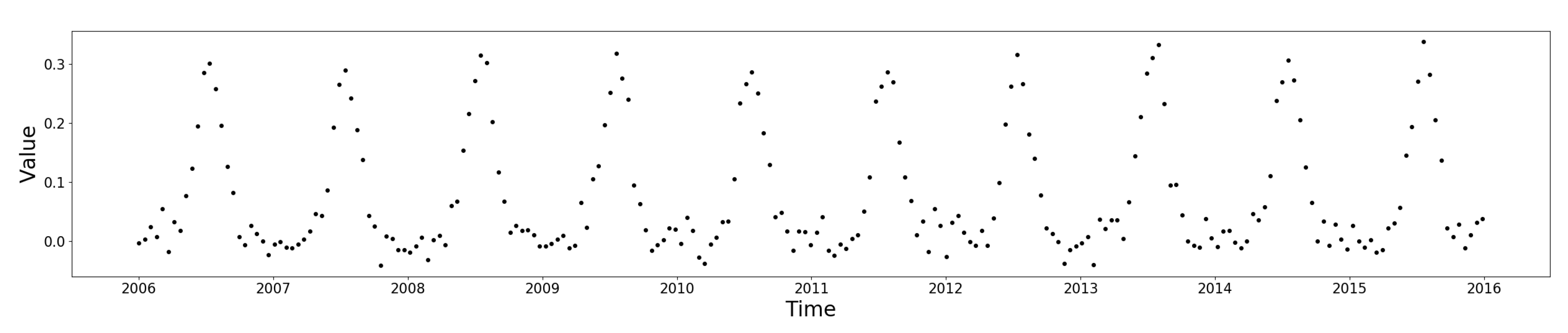
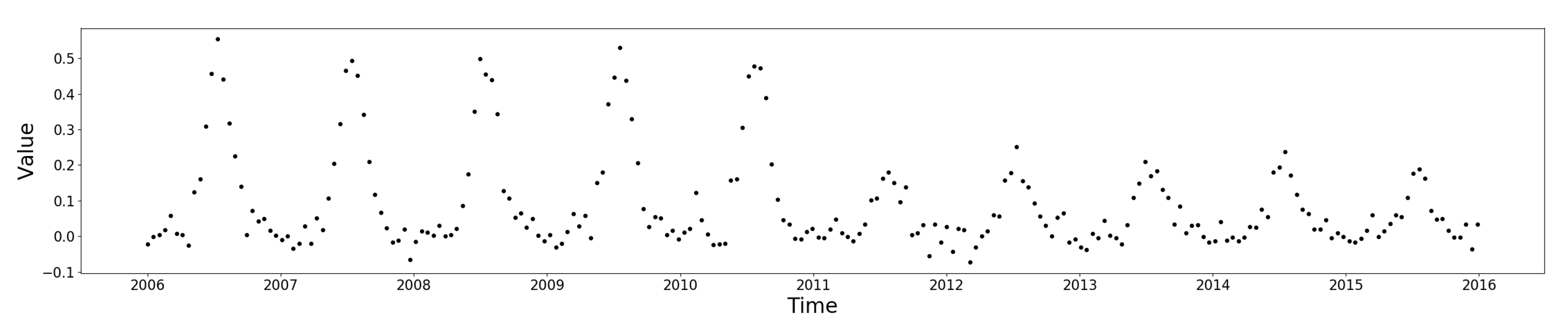
2.2. Simulating Seasonal Time Series

The method used to generate the simulated NDVI time series was based on that described by Verbesselt et al. [15,24]. We chose to simulate NDVI because most of the methods are designed to work on a single band or index. Furthermore, NDVI is a well-recognised and widely used metric for examining trends in vegetated areas. The method involves using a double Gaussian function to simulate an NDVI signal over time, where t = 1 , …, t = n for a time series with n observations per year. For each year in the time series, the NDVI value at time t is defined by the amplitude of the seasonal curve (a) (i.e., the peak NDVI value), the base or lowest winter value, the location in time of the maximum value for each year b, the width of left left hand side of the curve ( c 1 ), and the width of right hand side of curve ( c 2 ) (Equation (2)). Based on work by Verbesselt et al. [15], we used a value of b = 12 to simulate 10-year time series at a 16-day temporal resolution giving approximately 23 observations per year and centering the curve around the middle of the year. The trend component is a small NDVI value which is added or subtracted cumulatively from each value, to create an upward or downward trajectory. The noise component was added randomly to create more realistic variation in the time series, as explained in Section 2.3.
The amplitude and width of the generated seasonal curve can therefore be altered by using the parameters a, c 1 , and c 2 . Increasing the value of c 1 results in a corresponding increase in Start of Season (SOS), as shown in Figure 1. The method described by White et al. [35] was used to calculate number of days by which the start of season had moved forward for the corresponding change in c 1 (Table 1).
f ( t ; a , b , c 1 , c 2 ) = a × b a s e + e x p [ ( t b ) 2 / c 1 ] + t r e n d + n o i s e , if t > b b a s e + e x p [ ( t b ) 2 / c 2 ] + t r e n d + n o i s e , if t < b

2.3. Noise

The presence of noise is inevitable in satellite image time series of optical data. Atmospheric and sensor effects can lead to random variation, which is difficult to screen out. Robustness to noise is therefore important when considering which change detection method to use. Noise was added to the NDVI time series by randomly drawing a value from a normal distribution with a mean of 0 and a standard deviation of 0, 0.01, 0.02, …, 0.07, meaning that a simulated time series with a noise level of 0.02 will have a random number between −0.02 and 0.02 added to each individual NDVI value. Therefore, it should be noted that simulations with higher noise levels have noise added from a wider distribution, and therefore contain both a wider variance of noise and higher individual noise values on average. Fifty simulations were generated for each level of noise in order to avoid any bias caused by noise being unevenly distributed throughout the time series (e.g., higher levels of noise being concentrated at the start of the time series).

2.4. Missing Data

Satellite image time series are rarely complete. The presence of contaminants such as clouds, cloud shadows, and snow causes anomalous values which can be detected and removed to some degree, leaving gaps. As with noise, robustness to missing data is therefore a crucial component of evaluation when considering change detection methods, especially when applying change detection to parts of the world with persistent cloud or snow cover.
Data were removed from each simulated time series by first calculating the number of observations to drop based on the length of the time series and the percentage data missing. This was rounded up to the nearest integer. A random number generator was then used to select observations based on their index in the time series. If an index came up more than once, the duplicate was discarded. NDVI values for the randomly selected indices were then removed. Fifty simulations were generated for each level of missing data to avoid any bias caused by missing observations being unevenly distributed throughout the time series.

2.5. No Change Set

A set of simulations was generated where no change occurred. This was done to assess how likely the different methods were to detect a change where none existed. These simulations maintain a consistent seasonal cycle throughout (Figure 2). The no change set consists of 2400 simulations (50 replicates for each of eight levels of noise and for each of five levels of missing data) (Table 2).

2.6. Trend Only Set

A set of simulations was generated which contains a constant negative or positive trend, but no other changes. This was done to assess how likely the different methods were to detect an abrupt change where none existed, if a constant trend was present in the time series. Long-term trends are often present for vegetative land cover types, for example, due to land degradation [36] or the effects of global warming [16]. However, apart from EWMACD, all of the methods used in this study incorporate a trend term in the fitted model and are designed to flag only abrupt (step) changes or seasonal changes.
The trend only set consists of 14,400 simulations. Simulations were generated for six levels of trend (Table 2).

2.7. Seasonal Change Sets

A set of simulations was generated which contains a change in the shape of the seasonal curve. This was done to assess how well the different methods detect subtler changes in time series, in addition to abrupt/step changes. Given that all methods fit a seasonal component, it would be expected that fitted models would break down given a change in amplitude or Length of Season (LOS) because this would alter the fit of the model. However, BFAST is the only method which delineates seasonal changes from trend changes. The three seasonal change types are a change in the amplitude of the seasonal cycle (Figure 3), a change in the LOS, and a change in the number of seasons (i.e., from one peak per year to two) (Table 2). These simulation types were designed to imitate various changes in land productivity. For example, a change in seasonal amplitude or SOS (Start of Season) could indicate greater yield or an earlier planting, whereas a change in number of seasons simulates a change in number of yearly cropping cycles. The magnitude of the seasonal changes used was based on previous work by Verbesselt et al. [15,24,37].

2.8. Break/Trend Set

A set of simulations was generated which contains different magnitudes of abrupt change followed by different levels of trend. This was done to simulate changes that occur from sudden events such as logging, fire, or flood, which may be followed by longer term recovery or degradation of vegetation. Different levels of trend were included because, while a trend should not be detected as a change in itself (except in the case of EWMACD), the presence of a trend after a break contributes to how easily the break is detected, especially if there is noise or missing data. For example, a low-magnitude positive abrupt change will be easier to detect if it is followed by a steep positive trend, because, even if the initial event is missed, the time series will continue to deviate significantly from the previous stable period. However, an abrupt drop followed by fast recovery, such as is shown in Figure 4, might be more difficult to detect because there is substantial overlap of the values from before and after the break.

2.9. Definition of Change

For the break/trend set, a correct change is defined as a change detected by the algorithm 96 days or less (equating to six observations, or roughly three months) after the date of the true break. Changes are always placed at the start of 2011 such that the earliest possible date the change could be detected given the data frequency is the 15 January 2011. Given that the purpose of this study is to investigate the efficacy of these methods when applied to dense time series, detecting an abrupt change within a quarter of a year was considered a reasonable expectation. For the seasonal change sets, a correct change is defined as a change detected within one year (23 observations or 368 days), since changes in the shape or length of seasons are only of interest on a yearly basis.

2.10. Correlation Statistics

Correlation statistics were calculated using the non-parametric Spearman’s rank measure. Spearman’s ρ statistic provides an indication of the monotonic relationship between two variables (i.e., whether both variables increase or decrease together when ranked).

2.11. Computer Specifications and Timing

All steps including generation of simulations, production of results, and analysis were carried out on using a desktop computer with an Intel i7 CPU running at 4.20 GHz with 32 GB of RAM. Total runtime using a single process was recorded for each simulation set for each method. This total was then divided by the number of simulations in the set in order to obtain a mean runtime per simulation in seconds.

3. Results

3.1. Runtime

There was a lot of variation in how quickly the different methods processed the simulations. Table 3 shows that the sets with no changes generally took less time to process than those with changes, except for in the case of CCDC with CV, where they took longer. BFAST also took less time to process time series with NOS changes than those with no changes at all. There is a clear difference between CCDC and CCDC with CV, with the latter taking on average more than 1 s longer per simulation. There is also a difference between BFAST and BFAST Monitor, with BFAST being on average much slower. EWMACD and BFAST Monitor performed similarly in terms of mean time per simulation but BFAST Monitor was less variable and slightly faster.

3.2. Overall Summary

3.2.1. Definition of Correct/False Trend Results for EWMACD

Since EWMACD does not include a trend term, it flags condition (trend) changes as breaks. Therefore, a correct result for EWMACD for the trend only set is defined as a result where EWMACD detected at least one break. A specific number of breaks was not used because how often EMWACD flags a trend as a change depends heavily on the parameters used and the steepness of the trend. For example, Figure 5A shows the results of an initial run of EWMACD on a time series with a trend of 0.001. Since the trend in the data is not accounted for, the fitted model deviates fairly quickly from the real data and a change is quickly flagged in June 2008. After re-initialising, EWMACD flagged another change in February 2013. Figure 5B shows the result for a time series with a trend of 0.002. Due to the steeper slope, EWMACD detected five breaks in this time series overall, the maximum possible given the two-year training period. For these reasons the results for the trend only set for EWMACD in Table 4 for false breaks were excluded since there is no definition of a false break for EWMACD for that set.
Additionally, for the break/trend set, breaks detected after the specified temporal window for correct break detection (96 days) are not counted as false breaks for EWMACD in cases where a trend greater than zero follows the break. While these constraints may produce a positive bias for EWMACD in terms of false break detection, this was considered to be the fairest way to maintain comparability between EWMACD and the other methods as it does not require EWMACD to be parameterised differently for different simulation types.

3.2.2. True vs. False Changes
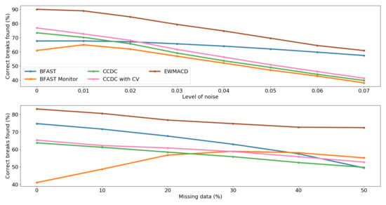
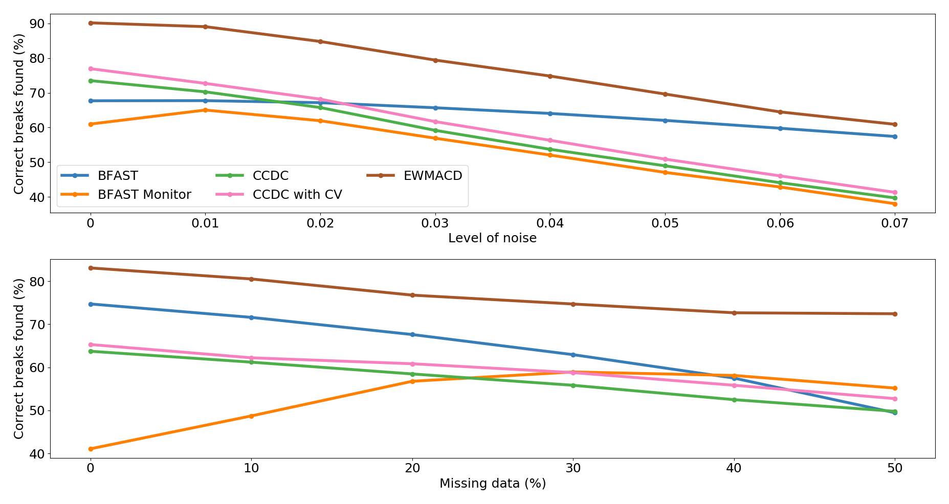
Table 4 provides an overall view of how each method performed on the different simulation sets. Results are presented as the percentage of simulations for that set for which the method either correctly identified there was no break (for the no change and trend only sets), or correctly identified a break within the specified temporal window (for the seasonal and break/trend sets). When considering Table 4, it is worth noting that, because all results are given as a percentage of the number of simulations in that set, the break/trend set contains 66% of all simulations and therefore performance in this set provides the best indication of overall method performance.
EWMACD gave the best performance in terms of overall effectiveness at break detection, correctly identifying a break where one existed in 76.6% of cases (i.e., excluding the no change and trend only sets). BFAST gave the second best performance (61.8%), followed by CCDC with CV (54.8%), BFAST Monitor (54.7%), and finally CCDC (51.8%). For false break detection (across all simulation sets), CCDC gave the best performance, detecting at least one false break in only 20.3% of simulations. For both the no change and trend only sets, CCDC correctly identified no break in nearly 100% of cases (Table 4). EWMACD gave the second best performance for false break detection overall (23.4%) and outperformed all other methods for the break/trend set (Table 4). However, performance on the three seasonal change sets was substantially worse than the other sets (Table 4). We looked at the distribution of false breaks for these sets, where changes detected before the true date of change were counted as premature changes and changes detected more than one year after the true date of change were counted as late changes. For the amplitude change set, EWMACD detected at least one premature change in 8.1% of simulations and at least one late change in 33.8% of simulations. For change in LOS, the figures were 8.3% and 33.3%, respectively. For change in NOS, they were 17.9% and 37.1%, respectively.
CCDC with CV gave the third best performance (26.1%) and was slightly more likely to detect breaks in the no change and trend only sets than CCDC (Table 4). This was followed by BFAST which detected at least one false break in 30.5% of all simulations. However, while BFAST performed less well than CCDC and CCDC with CV in the no change and trend only sets, it still only detected breaks in those sets around 20% of the time.
BFAST Monitor gave the worst performance in terms of false breaks, detecting at least one false break in 50.9% of simulations. Table 4 shows that BFAST Monitor was more likely to detect a false break than any other method in four out of the six simulation sets and performed substantially worse than any other method on the no change and trend only sets. Given that the performance of BFAST Monitor on the no change and trend only sets was so poor, it was re-run on those sets using one harmonic term instead of two. Reducing the number of harmonics reduces the complexity of the fit, potentially leading to fewer false breaks. Using one harmonic did decrease the number of instances where at least one false break was detected to 42.7% for the no change set and 44.4% for the trend only set. However, using a single harmonic also decreased the percentage of correct breaks detected in the break/trend set from 57.8% to 51.1%, and increased the number of time series where at least one false break was detected from 50.7% to 53.9%.
BFAST Monitor outperformed all methods at identifying changes in NOS, and outperformed all methods except EWMACD at detecting changes in amplitude and LOS (Table 4). It found more correct breaks for the amplitude and change in LOS sets when the magnitude of the change was greater. For example, it detected 68.9% and 70.2% of breaks correctly for the 0.3 and −0.3 amplitude change values, respectively, but only 36.7% and 32.9% for the 0.1 and −0.1 change values. EWMACD showed a similar pattern, correctly identifying more than 70% of changes in amplitude for the 0.3 and −0.3 levels but less than 40% of changes for the 0.1 and −0.1 levels. For change in LOS, EWMACD detected only 5.0% of breaks correctly for Δ c 1 = 5 while BFAST Monitor performed slightly better at 9.5%. Performance for Δ c 1 = 30 was much better for both EWMACD (65.4%) and BFAST Monitor (51.2%).
In contrast to EWMACD and BFAST Monitor, the other three methods performed poorly on the seasonal change sets. BFAST consistently failed to detect seasonal breaks of any type. It was the least effective method for detecting the onset of changes in amplitude, LOS, or NOS, but did frequently report at least one false change in those simulation sets (Table 4). CCDC and CCDC with CV were both more likely to detect a correct change for the change in NOS set than for the other two sets, where they performed similarly to BFAST (Table 4). However, CCDC and CCDC with CV were more likely to detect at least one false break in the change in NOS set than in the change in amplitude or change in LOS sets, whereas for BFAST the opposite was true. In the case of the change in amplitude set, BFAST detected at least one false break more than 50% of the time (Table 4), higher than any other method.

3.3. By Noise Level

Figure 6 shows a breakdown of the results from Table 4 by noise level. RMSE number of breaks is also included here because it provides an idea of whether methods tend to detect more or less breaks overall given increasing levels of noise, regardless of whether those breaks are correct or false. A method which always detected one break would have an RMSE of zero; however, the method could still be poor at estimating the timing of the break.
Results for the trend only set for EWMACD are not included in the breakdown plots of noise/missing data. Instead, percentages reflect correct results/false breaks found within the remaining simulation sets. This is because there is no way to include the trend only set in the false break and RMSE number of breaks plots for EWMACD because there is no way to determine error. Given that the definition of a correct break for the trend only set for EWMACD is more lenient than for other methods, and that EWMACD correctly identified a break nearly 100% of the time, the trend only set was also excluded from the correct breaks plots in order to create a fairer comparison.
All methods reported a significant negative correlation between percentage of correct results found (across all simulations) and noise level ( p < 0.01 , ρ < −0.9). The decrease in percentage of correct results found between the lowest and highest noise levels was approximately 20% less for BFAST than for any other method (Figure 6), suggesting more consistent performance across noise levels in this metric than the other methods.
All methods apart from CCDC with CV also reported significant positive correlations between noise level and percentage of results where at least one false break was found ( p < 0.01 , ρ > 0.9 ). Generally, the results for this metric are very similar for CCDC, BFAST, and EWMACD. The results for BFAST Monitor follow a more extreme trend, increasing from 38.2% to 65.4%. At higher levels of noise BFAST Monitor was substantially more likely to detect at least one false break in a time series than any other method (Figure 6).
No significant correlation was found between noise level and RMSE number of breaks for BFAST or CCDC with CV. Figure 6 indicates that while BFAST did not have the lowest RMSE values, it remained very consistent across noise levels. While a significant positive relationship was reported for EWMACD ( p < 0.01 , ρ = 0.93 ), it was also relatively consistent across noise levels for RMSE.
Above a noise level of 0.03, RMSE number of breaks for EWMACD, CCDC, and CCDC with CV is very similar. However, CCDC with CV shows a complex relationship between RMSE number of breaks and noise whereby it is more likely to detect the correct number of breaks with either very low or very high noise levels (Figure 6). In contrast, RMSE for CCDC with a fixed λ increased substantially with noise, from 0.36 to 0.66; the largest increase of any method. This relationship was significant ( p < 0.01 , ρ = 1.00 ). Below a noise level of 0.03, CCDC reported the lowest RMSE for number of breaks of any method, indicating that at low noise levels it is the most likely to correctly estimate the number of breaks in a time series. There was therefore a large difference in RMSE number of breaks between CCDC and CCDC with CV at the lowest noise levels. A significant positive relationship was also found between RMSE number of breaks and noise level for BFAST Monitor ( p < 0.01 , ρ = 0.88 ), which performed less well than any other method except for at the lowest noise level where CCDC with CV was worse.

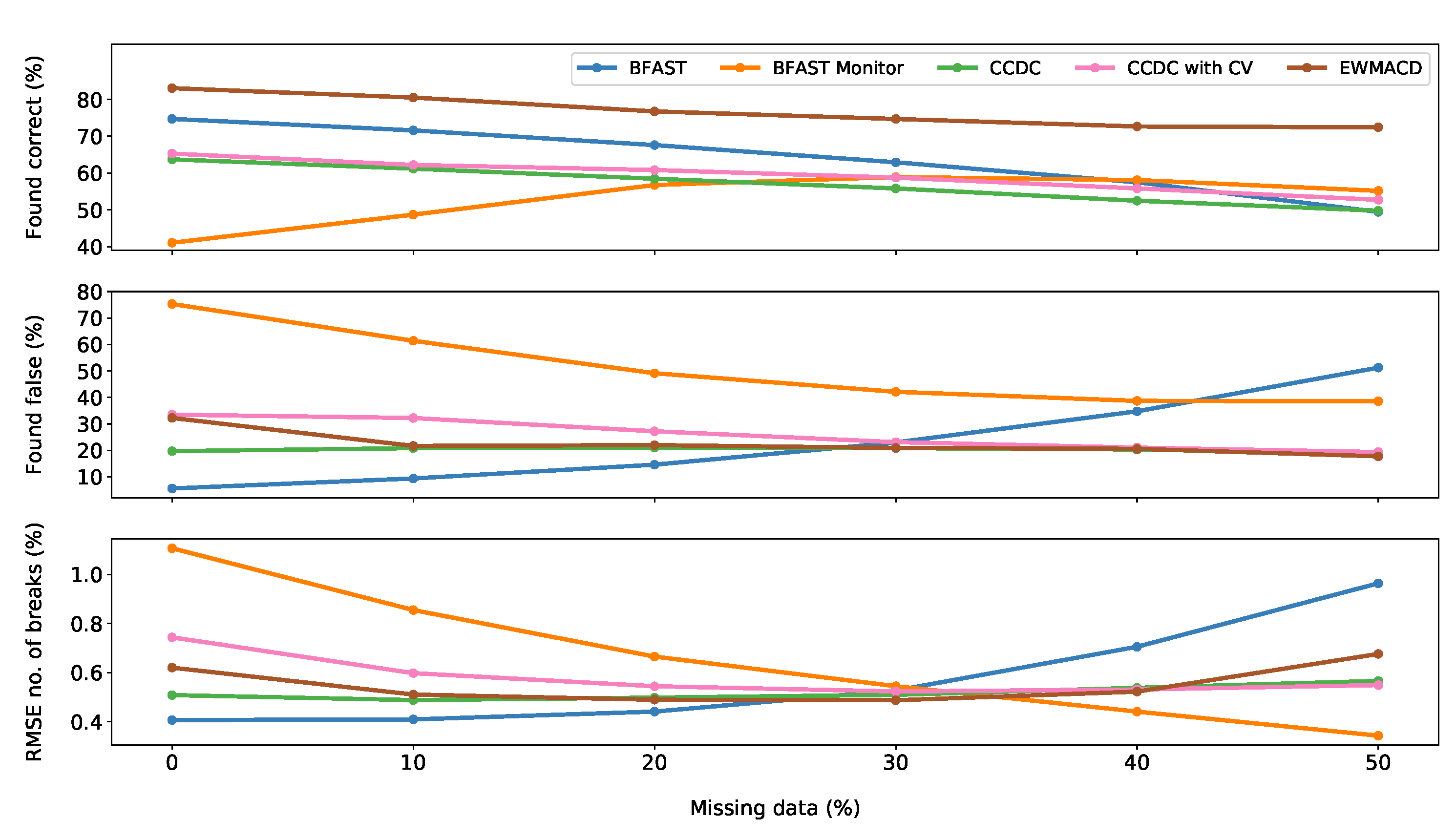
3.4. By Missing Data Level

Figure 7 shows a breakdown of the results in Table 4 by percentage of data missing. As with Figure 6, RMSE number of breaks is included here because it provides an idea of whether methods tend to detect more or less breaks overall given increasing levels of missing data, regardless of whether those breaks are correct or false.
Breaking down the results by percentage of missing data revealed contrasting trends for BFAST and BFAST Monitor. For BFAST, significant ( p < 0.01 ) positive correlations ( ρ = 1.00 ) were found between level of missing data and percentage of simulations where at least one false break was found and between missing data level and RMSE number of breaks. However, this was reversed for BFAST Monitor, where significant negative trends ( p < 0.01 , ρ = 1.00 ) were found for both metrics. A significant negative correlation ( p < 0.01 , ρ = 1.00 ) was also found for BFAST between missing data level and percentage of simulations where the correct break was found, whereas no significant trend was found for BFAST Monitor. Figure 7 shows an increasing trend for BFAST Monitor in terms of correct breaks found up to the 30% level, and then a slight decreasing trend. Overall, the results show that BFAST becomes less effective at break detection with more missing data, while BFAST Monitor becomes more effective.
CCDC with a fixed λ and CCDC with CV performed very similarly overall. Along with EWMACD, performance for these methods was more consistent than for BFAST and BFAST Monitor across missing data levels. Figure 7 indicates that, while CCDC was generally less likely to identify the correct break with increasing missing data, there was little effect of missing data level on the percentage of simulations where at least one false break was found or on RMSE number of breaks. This is confirmed by Spearman’s rank tests, which indicate a negative correlation of missing data level with percentage of correct breaks found ( p < 0.01 , ρ = 1.00 ) but no significant correlation of missing data level with the other two metrics. CCDC with CV also showed no significant correlation of missing data level with RMSE number of breaks and a significant negative correlation between missing data level and percentage of correct breaks found ( p < 0.01 , ρ = 1.00 ). However, Figure 7 indicates that CCDC with CV was more likely than CCDC to overestimate number of breaks for levels below 30%. Unlike CCDC, CCDC with CV showed a significant negative correlation between missing data level and percentage of results with at least one false break ( p < 0.01 , ρ = 1.00 ). Figure 7 indicates that this is due to CCDC with CV being more likely than CCDC to detect at least one false break for missing data levels below 40%.
As with CCDC and CCDC with CV, a Spearman’s test showed no significant correlation for EWMACD between missing data level RMSE number of breaks. Figure 7 shows that this is because EWMACD was better at estimating the number of breaks at very high and very low levels of missing data. There were significant negative correlations with percentage of true breaks detected and percentage of results where at least one false break was found ( p < 0.01 , ρ < 0.9 ). While both EWMACD and BFAST Monitor showed significant negative correlations between missing data level and percentage of simulations where at least one false break was found, the trend was much less pronounced for EWMACD (Figure 7). While a significant trend was found for percentage of correct breaks detected, EWMACD appears generally less affected by missing data for this metric than any other method (Figure 7).

3.5. Break Magnitude by Noise and Missing Data

Figure 8 shows RMSE break magnitude for each method by level of noise and by level of missing data, for all correctly identified breaks in the break/trend set. RMSE break magnitude was not investigated for the seasonal change sets because no method except BFAST was designed to estimate the magnitude of seasonal changes. Forty-three data points were removed from this dataset for BFAST Monitor because the estimated break magnitude for those breaks was extremely unrealistic and outside the possible range for a change in NDVI (i.e., a maximum change magnitude of ± 2 ). Given that the size of the dataset is 100,800 simulations, this represents a very small proportion of the data. Without these outliers, the RMSE break magnitude results are likely to be much closer to typical performance for BFAST Monitor.
All methods showed a significant positive correlation between noise level and RMSE break magnitude ( p < 0.01 , ρ > 0.95 ) using a Spearman’s rank correlation test. CCDC, CCDC with CV, and EWMACD showed no significant correlation between missing data level and RMSE break magnitude. However, BFAST and BFAST Monitor reported significant ( p < 0.01 ) positive ( ρ = 1.00 ) and negative ( ρ = 0.94 ) trends, respectively. It is clear in Figure 8 that CCDC and CCDC with CV performed almost identically at estimating break magnitude across all noise and missing data levels. EWMACD also produced a very similar result to the CCDC methods. BFAST consistently performed better than any other method, and BFAST Monitor consistently performed worse.

3.6. By Break Severity

To more closely investigate the ability of the different methods to detect different types of break, the break/trend set was broken down into three categories of break: Extreme, Moderate, and Subtle. This was not done for the seasonal change sets (change in amplitude, change in LOS, and change in NOS) because, as Table 4 indicates, results for those sets were generally poor. Simulations were categorised based on level of break and level of trend following the break, with the idea being that larger breaks followed by strong positive or negative trends are easier to detect than smaller magnitude breaks followed by weak trends or no trend at all. Break severity was therefore categorised as follows:
  • Extreme breaks have a large or medium magnitude break (break > 0.1 or break < −0.1) followed by a strong or medium trend (trend > 0.001 or trend < −0.001). n = 38,400 .
  • Moderate breaks have a large break (break = 0.3 or break = −0.3) with a weak trend (trend = 0.001 or trend = −0.001), a large break with no trend, a small break (break = 0.1 or break = −0.1) with a strong trend (trend = 0.002 or trend = −0.002), or a medium break (break = 0.2 or break = −0.2) with a weak trend (trend = 0.001 or trend = −0.001). n = 33,600 .
  • Subtle breaks have a small break (break = 0.1 or break = −0.1) with a weak trend (trend = 0.001 or trend = −0.001), a small break with no trend, a small break with a medium trend (trend = 0.0015 or trend = −0.0015), or a medium break (break = 0.2 or break = −0.2) with no trend. n = 28,800 .
As described in Section 3.5, when calculating RMSE break magnitude, 43 data points were removed from the dataset for BFAST Monitor. Table 5 shows all methods were less likely to detect the correct break in a time series as break severity decreased. The largest decreases were for CCDC and CCDC with CV, with differences of 44.4% and 42.2%, respectively, between the Extreme and Subtle simulation sets. In contrast, the reduction between these sets for EWMACD was around four times less at 10.5%.
All methods were more likely to detect at least one false break in a time series as break severity decreased (Table 5). The method with the largest increase between the Extreme and Subtle simulation sets was BFAST Monitor (18.6%). The method with the smallest increase was CCDC with CV (8.7%).
Table 5 also shows that, when considering breaks which were correctly identified, BFAST Monitor was 50% better at estimating the magnitude of Subtle breaks than Extreme breaks. For all other methods, the change in RMSE magnitude between the Extreme and Subtle change sets was 0.01 or less.

4. Discussion

4.1. BFAST

BFAST is a widely used method and a recent study by Saxena et al. [11] found that it rarely failed to detect breaks in time series. We found that, for simulations with a change, BFAST correctly identified more changes than any method other than EWMACD. It was also the most accurate method for estimating the magnitude of breaks and performed fairly consistently across noise levels. BFAST estimates break magnitude using the models fitted both before and after the break, which is more difficult for live monitoring methods which cannot fit a new stable model until multiple new observations are available. Given that BFAST receives the whole time series at once, it is also not unexpected that we found it to be more robust to noise than the live monitoring methods, which are more likely to be influenced by a single noisy data point. BFAST also performed relatively consistently across a range of different change severity levels for the break/trend set.
Given that BFAST uses an iterative process to find breaks, it is not unexpected that we found it to be slower than other methods at processing time series. BFAST was faster when applied to the simulations with no real changes. This was probably because BFAST first evaluates the possibility of any change being present using the OLS-MOSUM test. Optimisation of breakpoints is only carried out if the OLS-MOSUM test indicates a structural change within the time series.
BFAST appeared to be more affected by missing data than other methods. Unlike all other methods, BFAST was more likely to detect at least one false break the more data were missing and more likely to incorrectly estimate the number of breaks overall. A possible reason for this is the linear interpolation used to create a daily time series for processing with BFAST. The more data are removed, the less well this interpolation will represent the true temporal trajectory of the data. This is one possible explanation for BFAST’s high likelihood of detecting at least one false break in this study.
BFAST is the only method we used which explicitly aims to detect seasonal changes separately from trend changes [15]. However, we found that BFAST performed very poorly at detecting seasonal changes such as a change in amplitude, change in LOS, or change in the number of seasons. This poor performance existed across all magnitudes of change for the change in amplitude and change in LOS sets. A possible explanation is that these changes are too easily accounted for by the trend component. Given the whole time series at once, BFAST attempts to fit the optimal number of breakpoints to both the trend and seasonal component. However, as seen in Figure 9A, a decrease in signal amplitude results in an overall decrease in NDVI and can be interpreted as a break in trend. In Figure 9B, the change in LOS has been interpreted as a trend across the time series and no break is detected. The tendency of BFAST to account for amplitude and LOS changes by assuming a steeper trend is probably why BFAST was more likely to report at least one false break in this simulation set (Table 4), since trend breaks were not counted as correct for seasonal breaks even if they were temporally correct.
BFAST detected very few changes in NOS correctly. Figure 9C shows that BFAST could, on some occasions, correctly detect this type of change. However, in some cases, BFAST simply fitted a more complex seasonal model to the entire time series. The effect of this can be seen in Figure 9D.

4.2. BFAST Monitor

BFAST Monitor was the fastest method and the most consistent in average runtime across simulation types. Overall, it came second to last at correctly identifying breaks in time series where they existed; only CCDC performed worse. BFAST Monitor also consistently detected more breaks than were present in the time series. This may explain to some extent why BFAST Monitor was so poor at finding true breaks; if a false break is detected in the two years before the true break, the true break is likely to be missed when re-initialising with a new stable history period.
We considered that BFAST Monitor’s high false break detection rate might be a result of the second-order harmonic model overfitting the data. Previous studies have used a single harmonic model with BFAST Monitor in areas with low observation frequency where the underlying data were known to follow a simple seasonal curve [25,38]. However, while using a simpler model did reduce the number of time series where at least one false break was detected for the no change and trend only sets, it increased it for the break/trend set. This indicates that a single-order harmonic model was too simple for the underlying data. The second-order harmonic we used for BFAST Monitor was also the same order as that used for EWMACD, which was far less likely to detect at least one false break for the no change set. Given that EWMACD does not incorporate a trend term, it is possible that BFAST Monitor simply has more dimensions in which to overfit.
BFAST Monitor performed similarly to EWMACD on the seasonal change sets and better than BFAST, CCDC, or CCDC with CV. Given that BFAST Monitor was better at detecting larger magnitude changes for the amplitude and change in LOS sets, there is evidence that it can correctly identify seasonal changes, especially if they are large. However, BFAST Monitor performed worst overall at estimating the number of breaks in a time series. Alongside the high false break detection rates, this suggests that often even when BFAST Monitor does detect a break correctly, it will detect other non-existent breaks in the same time series.
Interestingly, BFAST Monitor was the only method which improved substantially the more data were missing. While this trend is less pronounced for percentage of correct breaks detected, it is clear that BFAST Monitor becomes both less likely to detect at least one false break and more likely to correctly estimate the number of breaks present with increased missing data (Figure 7). This is contrary to what we would generally believe, i.e. that more data equal better break estimation. Given this result, it could be concluded that BFAST Monitor is preferable to the other methods in regions with high quantities of missing data, e.g. regions with high cloud cover. However, given its high rate of false break detection, removing data may simply remove opportunities for breakpoints since BFAST Monitor operates on an observation-by-observation basis. Unlike the other live monitoring methods, the MOSUM method used by BFAST Monitor only requires a single observation to exceed a boundary for a change to be flagged [24,39]. While this allows for faster detection of breaks, it can lead to far more observations being flagged as changes.
In terms of estimating break magnitude, BFAST Monitor performed poorly, being the least accurate of all the methods (Figure 8). However, there was around a 50% improvement in RMSE break magnitude between the Extreme and Subtle change sets for the break/trend simulation set, suggesting that BFAST Monitor struggles to accurately estimate larger breaks. This is possibly because the method used by BFAST Monitor to estimate break magnitude is based on median values. For breaks followed by strong trends, this could result in break size being underestimated as in Figure 10A, or overestimated as in Figure 10B, because the trend component causes the median of the trend segment to move closer to or further away from the values of the first segment. It could be argued that BFAST Monitor is actually providing more information about the change here because break magnitude is influenced by the direction of recovery. The usefulness of that additional information will depend on the intention of the study being undertaken.

4.3. CCDC

CCDC ranked in the middle for runtime, being much faster than CCDC with CV and BFAST but slower than BFAST Monitor and EWMACD. Overall, CCDC detected at least one false break in the fewest number of time series, but was worse than any other method at identifying changes where they existed. Based on this study, the main strength of CCDC is that it is unlikely to overestimate the number of breaks. However, this comes at the cost of also being more likely to miss breaks where they exist. It must be borne in mind that the purpose of CCDC is to detect complete changes in land cover type. While the classification element of CCDC was not discussed here, its lack of sensitivity to smaller changes might be a positive in this regard. The emphasis on changes in class is also probably why CCDC performed so poorly at detecting seasonal changes. A change in land cover class is likely to result in more complex changes to the shape of the seasonal curve than a straightforward change in amplitude or LOS.
There is evidence for this in the observation that CCDC did detect more breaks, both correct and false, in the NOS change set than in the change in amplitude or change in LOS sets. Since CCDC uses the RMSE of models to find changes, if a model underfits the seasonal curve, then many seasonal changes may not exceed the six times RMSE level required for CCDC to confidently flag a change. Figure 11A and Figure 12A show that CCDC sometimes failed to properly capture the amplitude and shape of time series. A change in the number of seasons introduces changes at the start, end, and middle of the season; multiple points at which the previous model can fail to fit.
We considered that the tendency of CCDC to underfit was due to the value of λ = 0.01 , which we selected. However, CCDC with CV did not perform substantially differently to CCDC, leading us to believe that the Lasso fitting method is generally more likely to underfit the seasonal curve than OLS fitting. This makes it a suitable choice if the aim is to detect only the more substantial changes in a time series. CCDC also detected around 50% fewer breaks in the Subtle change category compared to the Extreme change category for the break/trend set, suggesting that CCDC is also unlikely to detect more minor breaks or trend changes which again could be associated to within-class rather than between-class changes. However, CCDC with fixed λ may provide more opportunity to control the degree of over- or underfitting. Given the increase in speed over using cross validation, we would suggest that using a fixed value for λ is preferable if the value is chosen carefully.
CCDC became substantially worse at estimating the number of breaks and detecting correct breaks (or correct absence of breaks) with increasing noise level, although percentage of simulations where at least one false break was detected did not increase (Figure 6). This suggests that, as noise increases, CCDC is more likely to miss breaks altogether rather than attributing an incorrect date of change. Both percentage of results where at least one false break was found and RMSE number of breaks for CCDC were stable across missing data levels. Therefore, the evidence is that noisy data are more likely to affect the efficacy of CCDC in correctly identifying breaks than missing data. This supports the conclusion that CCDC is more suited to situations requiring robust identification of complete changes in land cover, as it is unlikely to flag smaller changes in noisy time series.
CCDC, CCDC with CV, and EWMACD all performed very similarly at estimating break magnitude; this was expected given that the same method was used for all three. In general, this method of break estimation appears to be robust to missing data but does get less effective with increased noise. The effect of noise is not surprising given that this method relies on residual values; the more noisy the data are, the less likely that value is to reflect the true break size. The method used by BFAST had much lower RMSE and was more robust against noise.

4.4. CCDC with CV

The purpose of using a cross-validated approach was to investigate whether allowing λ to vary would produce substantial improvement over a fixed λ . Not surprisingly given that cross-validation requires fitting large numbers of models, CCDC with CV took much longer to run than the other methods.
Overall, we found that using CV made CCDC more likely to detect true breaks, but also more likely to detect at least one false break in a time series. This suggests that using a cross-validated approach did lead to more closely fitting models than using λ = 0.01 and to overfitting in some cases. Figure 12 shows an example where CCDC with CV detects two additional breaks where CCDC estimates the number of breaks correctly.
One observation we made was that, unlike CCDC, CCDC with CV did not have a straightforward relationship between RMSE number of breaks and noise. CCDC with CV was found to be less accurate at detecting the number of breaks at the lowest and highest noise levels than at the intermediate levels. With increased noise, the method was less likely to detect correct results and the likelihood of detecting at least one false break remained constant. However, the change in RMSE tells us that the actual number of false breaks found is likely to be higher at extremes of noise. At high levels of noise, models are more likely to be influenced by noisy data points and may be fitting to noise. This means that more false breaks get detected, but fewer true breaks. This is probably why most of the methods performed less well in terms of RMSE number of breaks at high noise levels. The unique pattern shown by CCDC with CV suggests that it must also be detecting more breaks if there is very little noise. With less noise, CCDC with CV may be fitting the data too closely, leading to more false breaks per simulation.
CCDC with CV was slightly more likely to overestimate the number of breaks and more likely to detect at least one false break in a time series than CCDC at missing data levels less than 40%. These trends are much less pronounced than for BFAST Monitor, and since CCDC requires six observations to confidently flag a change, the cause is likely to be different. In the case of CCDC with CV, we believe that this effect is probably again due to a tendency to overfit; with fewer data, CCDC with CV has fewer points to fit to. Figure 11B shows the output from CCDC with CV for a time series with no breaks and very few missing data, where the algorithm detects a non-existent break.
CCDC with CV performed similarly to CCDC in the breakdown by change severity. One notable difference is that CCDC with CV was more likely to correctly identify breaks in the Subtle change category, and was more likely overall to detect at least one false break in a time series. This reinforces the previous point that while in general CCDC is not designed to detect lower magnitude changes, some control over sensitivity can be gained by setting the value of λ appropriately. Lasso fitting attempts to regularise the model coefficients, in some cases reducing them to zero, resulting in a form of feature selection. Larger values of λ will increase the degree of regularisation and therefore increase the likelihood that some seasonal coefficients will be reduced to zero. CCDC was never intended to be able to detect seasonal breaks [28,29,31] and therefore it is not unexpected that both CCDC variants performed poorly on these simulation sets.

4.5. EWMACD

EWMACD is designed to detect subtler changes, such as partial disturbance of forest pixels [32]. This claim is supported by the results of the simulation testing. Across all simulations with a change, EWMACD was by far the most effective at correctly identifying the date of change. The high overall rate of correct change estimation is due to EWMACD’s good performance across both the break/trend and seasonal change sets. While EWMACD was not able to detect all seasonal changes, overall it outperformed any other method. For higher magnitudes of seasonal change, EWMACD performed very well at correctly identifying changes. Figure 13A shows how a change in amplitude results in deviation from the history period, causing deviation in the control chart around the peaks of the seasonal curves.
Across all simulations, only CCDC was less likely to detect at least one false break. However, EWMACD was much more likely to detect false changes in seasonal sets than in other sets. It must be remembered that, for the break/trend set, any changes after the 96-day window were not counted as false for EWMACD because it is designed to detect trend changes. The lower likelihood of detecting at least one break in a time series for the break/trend set is probably because of this. However, EWMACD only detected a change in the no change set around 20% of the time. We also found that EWMACD was around three times more likely to detect a false break after the date of true change as before. This suggests that the higher rate of false change detection in the seasonal change sets might partly be caused by changes being detected too late, as shown in Figure 13B. It is also possible that the vertex method used to find the next stable period after a change does not work as well for seasonal changes where the historic model still fits some parts of the seasonal curve.
EWMACD’s response to noise was as expected in that, the noisier are the data, the less likely EWMACD was to correctly identify the number and location of breaks. At noise levels less than 0.03, only CCDC performed better in terms of RMSE number of breaks. At high noise levels, EWMACD was still more likely to correctly identify a break (or lack of one) than any other method. As with CCDC and CCDC with CV, break magnitude estimation got worse with noise, but not with missing data, as discussed in previous sections.
EWMACD did show an unusual result for response of RMSE number of breaks to missing data level, whereby RMSE was higher for the 0 and 50% levels than for the levels in between. EWMACD was also more likely to detect at least one false break with no missing data than at any other level, although this evened out over the remaining levels. Percentage of correct results had an overall downward trend. This suggests that, when there are no missing data, EWMACD is detecting too many changes, whereas, at the 50% missing data level, it is detecting too few. This is possibly because if more data are available, EWMACD is more likely to overfit the data than the CCDC methods, which are closest to EWMACD in trend. With 50% of the data missing, EWMACD may reach a tipping point where it lacks enough data to adequately fit the model, leading to a less well fitting model and making change detection more difficult.
EWMACD had the second fastest runtime behind BFAST Monitor, although runtime was more variable than for CCDC or for BFAST Monitor. The increased variability was partly because runtime on the trend only set was higher than the other sets due to EWMACD detecting more changes and therefore needing to output more results. Given that EWMACD performed far better at break detection than BFAST Monitor we conclude that for seasonal breaks and subtler abrupt changes it is the preferred method.

4.6. Limitations

The authors recognise that using simulated data in place of real-world observations has its limitations. The simulations used in this study are essentially idealised time series as it is very difficult to realistically simulate the levels of variation that exist in the real world. This will bias results towards being over-optimistic, and all of the methods studied will likely perform less well on real-world data. However, we carried out very little optimisation in an attempt to keep the methods as comparable as possible. Some result are therefore likely to be negatively biased in comparison to more specific real-world applications. To facilitate comparability and examine off-the-shelf performance, this study used parameters which were not optimised for the the presented problems. In many cases, real data will also contain multiple breakpoints; however, assuming a sufficient stable period between changes, accuracy would likely be very similar across all breakpoints.

4.7. Future Work

We believe that simulated data enable a robust way of evaluating different change detection approaches under a range of scenarios, which would not be possible using real data. Using simulations can provide a benchmark against which to test new methods as well as an objective way to compare different methods and determine their strengths and weaknesses. Simulations could also be used when proposing new methods of quantifying change detection accuracy such as that proposed by Tang et al. [40].
A possible improvement to the simulated datasets used in this study would be to include more realistic year-to-year and seasonal variations. For example, seasonal cycles are likely to have yearly variations in amplitude, length, and shape due to fluctuating weather conditions or variations in yield. We also distributed noise evenly throughout the year, whereas in reality noise caused by factors such as cloud contamination tend to be clustered around certain times of year.
In addition to creating more realistic simulations, there is also potential to use simulated data to better explore the limitations of individual methods. Many methods have multiple parameters that must be set by the user. While expert knowledge of the study area can be used to decide these values, simulations can support this knowledge by allowing the user to test how different parameters might cause an algorithm to behave differently under different scenarios. Simulations can also be parameterised to better reflect specific study areas or vegetation types [15,16,24]. This type of customisation could also be improved using the suggestions given above, for example, by estimating how much year-to-year seasonal variation should be expected in vegetation by using climate data.
The simulations used in this study provide a starting point for future studies and have been made available for download [41].

5. Conclusions

We present a novel means of robustly evaluating and comparing change detection techniques using simulated time series data. This firstly allows for each method to be evaluated against a wide range of change scenarios, including those where data are noisy or incomplete. Secondly, this process allows for comparison between methods based on temporal accuracy, likelihood of detecting false changes, and RMSE number of breaks. The insights gained can be used to provide recommendations for users as to which method might be most appropriate for their application. However, due to the limitations of this study, it is important to emphasise that further investigation and optimisation should be carried out to ensure the efficacy of any method when applied to a specific use-case. In particular, the selection of input parameters such as the order of the seasonal component, the number of breakpoints to detect, the length of the history period, and the value of λ for CCDC and EWMACD will have a substantial impact on the results achieved and in many cases default values will not be the most appropriate.

Recommendations

  • For smaller magnitude changes such as partial forest harvesting within pixels and for detecting changes in land cover condition (e.g., due to decreasing yield or recovery after fire), EWMACD is likely to be the most effective due to its ability to detect a wide variety of change magnitudes and low false detection rate.
  • For studies which aim to robustly detect complete changes in land cover class (e.g., change from forestry to cropland), we recommend CCDC with a fixed λ . CCDC performed well at detecting larger magnitude changes and tended to ignore or underestimate smaller magnitude changes and seasonal changes. Using fixed λ greatly increases algorithm runtime, although λ should be chosen carefully in order to maximise or minimise change detection as appropriate.
  • The detection of seasonal changes is a field in itself and software packages such as TIMESAT [42,43] can aid in more detailed reconstruction of seasonal curves. However, of the methods investigated here, we found both EWMACD and BFAST Monitor capable of detecting at least high magnitude seasonal change, such as a change in the number of seasonal peaks present (indicating a change in cropping practices) or a substantial increase in seasonal amplitude (indicating, e.g., a change in yield). Of the two, we would recommend EWMACD due to its lower likelihood of detecting false change.
  • If data are known to be noisy, e.g. with many small clouds or cloud shadows present which are difficult to screen out, either EWMACD or BFAST could be suitable. EWMACD was able to find more correct breaks in time series regardless of the level of noise, whereas BFAST was the most consistent method across noise levels for all metrics. However, given the poor performance of BFAST on the seasonal change sets, its use is only recommended here for finding abrupt changes.
  • For datasets with high levels of missing observations such as those from areas of the world with high year-round cloud or snow cover, we would recommend CCDC. CCDC gave very consistent performance across missing data levels, probably because it is designed to look for land cover class changes and is less likely to be influenced by single outliers. The adaptive Lasso regression method should also help to correctly estimate seasonal parameters if data are missing.
  • As computing power increases, change detection techniques can be applied across larger and larger datasets. Most of the methods discussed here are now available on Google Earth Engine [44]. Initiatives such as the Open Data Cube show the potential of continental scale analysis [45]. However, pixel-level change detection is still computationally expensive. Based on its good overall performance and fast execution time across multiple change types, EWMACD shows potential for large scale analysis.

Author Contributions

Conceptualisation, K.A.-C.; methodology, K.A.-C.; software, K.A.-C.; validation, K.A.-C.; formal analysis, K.A.-C., P.B., A.H., and G.B.; investigation, K.A.-C., P.B., A.H., and G.B.; resources, K.A.-C. and P.B.; data curation, K.A.-C.; writing—original draft preparation, K.A.-C.; writing—review and editing, K.A.-C., P.B., A.H., and G.B.; visualisation, K.A.-C., P.B., and A.H.; supervision, P.B., A.H., and G.B.; project administration, K.A.-C. and P.B.; and funding acquisition, P.B. and A.H.

Funding

This research was funded by Knowledge Economy Skills Scholarships (KESS 2). KESS 2 is a pan-Wales higher level skills initiative led by Bangor University on behalf of the HE sector in Wales. It is part funded by the Welsh Government’s European Social Fund (ESF) convergence programme for West Wales and the Valleys.

Conflicts of Interest

The funders had no role in the design of the study; in the collection, analyses, or interpretation of data; in the writing of the manuscript, or in the decision to publish the results.

Abbreviations

The following abbreviations are used in this manuscript:
BFASTBreaks for Additive and Seasonal Trend
CCDCContinuous Change Detection and Classification
CUSUMCumulative Sum
CVCross Validation
EdynDynamic EWMACD
EWMACDExponentially Weighted Moving Average Change Detection
HANTSHarmonic Analysis of Time Series
LandTrendrLandsat-based detection of Trends in Disturbance and Recovery
LOSLength of Season
MOSUMMoving Sum
NDVINormalised Difference Vegetation Index
NOSNumber of Seasons
OLSOrdinary Least Squares
RMSERoot Mean Square Error
SOSStart of Season

References

  1. Tubiello, F.N.; Salvatore, M.; Ferrara, A.F.; House, J.; Federici, S.; Rossi, S.; Biancalani, R.; Condor Golec, R.D.; Jacobs, H.; Flammini, A.; et al. The Contribution of Agriculture, Forestry and other Land Use activities to Global Warming, 1990–2012. Glob. Chang. Biol. 2015, 21, 2655–2660. [Google Scholar] [CrossRef] [PubMed]
  2. van der Werf, G.R.; Morton, D.C.; DeFries, R.S.; Olivier, J.G.J.; Kasibhatla, P.S.; Jackson, R.B.; Collatz, G.J.; Randerson, J.T. CO2 emissions from forest loss. Nat. Geosci. 2009, 2, 737–738. [Google Scholar] [CrossRef]
  3. Roy, D.P.; Wulder, M.A.; Loveland, T.R.; Woodcock, C.E.; Allen, R.G.; Anderson, M.C.; Helder, D.; Irons, J.R.; Johnson, D.M.; Kennedy, R.; et al. Landsat-8: Science and product vision for terrestrial global change research. Remote. Sens. Environ. 2014, 145, 154–172. [Google Scholar] [CrossRef]
  4. Wulder, M.A.; Masek, J.G.; Cohen, W.B.; Loveland, T.R.; Woodcock, C.E. Opening the archive: How free data has enabled the science and monitoring promise of Landsat. Remote Sens. Environ. 2012, 122, 2–10. [Google Scholar] [CrossRef]
  5. Kennedy, R.E.; Yang, Z.; Cohen, W.B. Detecting trends in forest disturbance and recovery using yearly Landsat time series: 1. LandTrendr—Temporal segmentation algorithms. Remote Sens. Environ. 2010, 114, 2897–2910. [Google Scholar] [CrossRef]
  6. Hermosilla, T.; Wulder, M.A.; White, J.C.; Coops, N.C.; Hobart, G.W. An integrated Landsat time series protocol for change detection and generation of annual gap-free surface reflectance composites. Remote Sens. Environ. 2015, 158, 220–234. [Google Scholar] [CrossRef]
  7. Huang, C.; Goward, S.N.; Schleeweis, K.; Thomas, N.; Masek, J.G.; Zhu, Z. Dynamics of national forests assessed using the Landsat record: Case studies in eastern United States. Remote Sens. Environ. 2009, 113, 1430–1442. [Google Scholar] [CrossRef]
  8. Moisen, G.G.; Meyer, M.C.; Schroeder, T.A.; Liao, X.; Schleeweis, K.G.; Freeman, E.A.; Toney, C. Shape selection in Landsat time series: A tool for monitoring forest dynamics. Glob. Chang. Biol. 2016, 22, 3518–3528. [Google Scholar] [CrossRef]
  9. Zhu, Z. Change detection using landsat time series: A review of frequencies, preprocessing, algorithms, and applications. ISPRS J. Photogramm. Remote. Sens. 2017, 130, 370–384. [Google Scholar] [CrossRef]
  10. Roerink, G.J.; Menenti, M.; Verhoef, W. Reconstructing cloudfree NDVI composites using Fourier analysis of time series. Int. J. Remote. Sens. 2000, 21, 1911–1917. [Google Scholar] [CrossRef]
  11. Saxena, R.; Watson, L.T.; Wynne, R.H.; Brooks, E.B.; Thomas, V.A.; Zhiqiang, Y.; Kennedy, R.E. Towards a polyalgorithm for land use change detection. ISPRS J. Photogramm. Remote. Sens. 2018, 144, 217–234. [Google Scholar] [CrossRef]
  12. Cohen, W.B.; Yang, Z.; Kennedy, R. Detecting trends in forest disturbance and recovery using yearly Landsat time series: 2. TimeSync—Tools for calibration and validation. Remote Sens. Environ. 2010, 114, 2911–2924. [Google Scholar] [CrossRef]
  13. Dutrieux, L.P.; Verbesselt, J.; Kooistra, L.; Herold, M. Monitoring forest cover loss using multiple data streams, a case study of a tropical dry forest in Bolivia. ISPRS J. Photogramm. Remote. Sens. 2015, 107, 112–125. [Google Scholar] [CrossRef]
  14. Cohen, W.B.; Healey, S.P.; Yang, Z.; Stehman, S.V.; Brewer, C.K.; Brooks, E.B.; Gorelick, N.; Huang, C.; Hughes, M.J.; Kennedy, R.E.; et al. How Similar Are Forest Disturbance Maps Derived from Different Landsat Time Series Algorithms? Forests 2017, 8, 98. [Google Scholar] [CrossRef]
  15. Verbesselt, J.; Hyndman, R.; Zeileis, A.; Culvenor, D. Phenological change detection while accounting for abrupt and gradual trends in satellite image time series. Remote Sens. Environ. 2010, 114, 2970–2980. [Google Scholar] [CrossRef]
  16. Forkel, M.; Carvalhais, N.; Verbesselt, J.; Mahecha, M.D.; Neigh, C.S.; Reichstein, M. Trend Change detection in NDVI time series: Effects of inter-annual variability and methodology. Remote Sens. 2013, 5, 2113–2144. [Google Scholar] [CrossRef]
  17. Awty-Carroll, K. Scripts Used for Evaluating and Comparing a Range of Dense Time Series Change Detection Methods. Available online: https://github.com/klh5/season-trend-comparison (accessed on 12 November 2019).
  18. Verbesselt, J.; Zeileis, A.; Hyndman, R. Package ‘Bfast’. Available online: https://cran.r-project.org/web/packages/bfast/bfast.pdf (accessed on 29 April 2019).
  19. Schmidt, M.; Lucas, R.; Bunting, P.; Verbesselt, J.; Armston, J. Multi-resolution time series imagery for forest disturbance and regrowth monitoring in Queensland, Australia. Remote Sens. Environ. 2015, 158, 156–168. [Google Scholar] [CrossRef]
  20. Grogan, K.; Pflugmacher, D.; Hostert, P.; Verbesselt, J.; Fensholt, R. Mapping clearances in tropical dry forests using breakpoints, trend, and seasonal components from modis time series: Does forest type matter? Remote Sens. 2016, 8, 657. [Google Scholar] [CrossRef]
  21. Watts, L.M.; Laffan, S.W. Effectiveness of the BFAST algorithm for detecting vegetation response patterns in a semi-arid region. Remote Sens. Environ. 2014, 154, 234–245. [Google Scholar] [CrossRef]
  22. Che, X.; Feng, M.; Yang, Y.; Xiao, T.; Huang, S.; Xiang, Y.; Chen, Z. Mapping extent dynamics of small lakes using downscaling MODIS surface reflectance. Remote Sens. 2017, 9, 82. [Google Scholar] [CrossRef]
  23. Platt, R.V.; Manthos, D.; Amos, J. Estimating the Creation and Removal Date of Fracking Ponds Using Trend Analysis of Landsat Imagery. Environ. Manag. 2018, 61, 310–320. [Google Scholar] [CrossRef] [PubMed]
  24. Verbesselt, J.; Zeileis, A.; Herold, M. Near real-time disturbance detection using satellite image time series. Remote Sens. Environ. 2012, 123, 98–108. [Google Scholar] [CrossRef]
  25. DeVries, B.; Verbesselt, J.; Kooistra, L.; Herold, M. Robust monitoring of small-scale forest disturbances in a tropical montane forest using Landsat time series. Remote Sens. Environ. 2015, 161, 107–121. [Google Scholar] [CrossRef]
  26. Schultz, M.; Shapiro, A.; Clevers, J.; Beech, C.; Herold, M.; Schultz, M.; Shapiro, A.; Clevers, J.G.P.W.; Beech, C.; Herold, M. Forest Cover and Vegetation Degradation Detection in the Kavango Zambezi Transfrontier Conservation Area Using BFAST Monitor. Remote Sens. 2018, 10, 1850. [Google Scholar] [CrossRef]
  27. Murillo-Sandoval, P.J.; Hilker, T.; Krawchuk, M.A.; Van Den Hoek, J. Detecting and attributing drivers of forest disturbance in the Colombian andes using landsat time-series. Forests 2018, 9, 269. [Google Scholar] [CrossRef]
  28. Zhu, Z.; Woodcock, C.E. Continuous change detection and classification of land cover using all available Landsat data. Remote Sens. Environ. 2014, 144, 152–171. [Google Scholar] [CrossRef]
  29. Zhu, Z.; Woodcock, C.E.; Holden, C.; Yang, Z. Generating synthetic Landsat images based on all available Landsat data: Predicting Landsat surface reflectance at any given time. Remote Sens. Environ. 2015, 162, 67–83. [Google Scholar] [CrossRef]
  30. Deng, C.; Zhu, Z. Continuous subpixel mapping of impervious surface area using Landsat time series. Remote Sens. Environ. 2018. [Google Scholar] [CrossRef]
  31. Zhu, Z.; Zhang, J.; Yang, Z.; Aljaddani, A.H.; Cohen, W.B.; Qiu, S.; Zhou, C. Continuous monitoring of land disturbance based on Landsat time series. Remote Sens. Environ. 2019. [Google Scholar] [CrossRef]
  32. Brooks, E.B.; Wynne, R.H.; Thomas, V.A.; Blinn, C.E.; Coulston, J.W. On-the-fly massively multitemporal change detection using statistical quality control charts and landsat data. IEEE Trans. Geosci. Remote. Sens. 2014, 52, 3316–3332. [Google Scholar] [CrossRef]
  33. Brooks, E.B.; Wynne, R.H.; Thomas, V.A.; Blinn, C.E.; Coulston, J. Exponentially Weighted Moving Average Change Detection—Script and Sample Data. Available online: http://vtechworks.lib.vt.edu/handle/10919/50544 (accessed on 29 April 2019). [CrossRef]
  34. Brooks, E.B.; Yang, Z.; Thomas, V.A.; Wynne, R.H. Edyn: Dynamic signaling of changes to forests using exponentially weighted moving average charts. Forests 2017, 8, 304. [Google Scholar] [CrossRef] [Green Version]
  35. White, M.A.; Thornton, P.E.; Running, S.W. A continental phenology model for monitoring vegetation responses to interannual climatic variability. Glob. Biogeochem. Cycles 1997, 11, 217–234. [Google Scholar] [CrossRef]
  36. De Jong, R.; Verbesselt, J.; Schaepman, M.E.; de Bruin, S. Trend changes in global greening and browning: Contribution of short-term trends to longer-term change. Glob. Chang. Biol. 2012, 18, 642–655. [Google Scholar] [CrossRef]
  37. Verbesselt, J.; Hyndman, R.; Newnham, G.; Culvenor, D. Detecting trend and seasonal changes in satellite image time series. Remote Sens. Environ. 2010, 114, 106–115. [Google Scholar] [CrossRef]
  38. DeVries, B.; Decuyper, M.; Verbesselt, J.; Zeileis, A.; Herold, M.; Joseph, S. Tracking disturbance-regrowth dynamics in tropical forests using structural change detection and Landsat time series. Remote Sens. Environ. 2015, 169, 320–334. [Google Scholar] [CrossRef]
  39. Zeileis, A. A unified approach to structural change tests based on ML scores, F statistics, and OLS residuals. Econom. Rev. 2005, 24, 445–466. [Google Scholar] [CrossRef]
  40. Tang, X.; Bullock, E.L.; Olofsson, P.; Estel, S.; Woodcock, C.E. Near real-time monitoring of tropical forest disturbance: New algorithms and assessment framework. Remote Sens. Environ. 2019, 224, 202–218. [Google Scholar] [CrossRef]
  41. Awty-Carroll, K. Simulated NDVI Time Series Repository. Available online: osf.io/taf9y (accessed on 29 April 2019). [CrossRef]
  42. Jönsson, P.; Eklundh, L. Seasonality extraction by function fitting to time-series of satellite sensor data. IEEE Trans. Geosci. Remote. Sens. 2002, 40, 1824–1832. [Google Scholar] [CrossRef]
  43. Jönsson, P.; Eklundh, L. TIMESAT—A program for analyzing time-series of satellite sensor data. Comput. Geosci. 2004, 30, 833–845. [Google Scholar] [CrossRef] [Green Version]
  44. Gorelick, N.; Hancher, M.; Dixon, M.; Ilyushchenko, S.; Thau, D.; Moore, R. Google Earth Engine: Planetary-scale geospatial analysis for everyone. Remote Sens. Environ. 2017, 202, 18–27. [Google Scholar] [CrossRef]
  45. Lewis, A.; Lymburner, L.; Purss, M.B.J.; Brooke, B.; Evans, B.; Ip, A.; Dekker, A.G.; Irons, J.R.; Minchin, S.; Mueller, N.; et al. Rapid, high-resolution detection of environmental change over continental scales from satellite data—The Earth Observation Data Cube. Int. J. Digit. Earth 2016, 9, 106–111. [Google Scholar] [CrossRef]
Figure 1. Plot demonstrating how a change in the c 1 parameter of Equation (2) results in a corresponding change in SOS. Here, the SOS has been moved forward by 37 days by changing the c 1 parameter from 5 to 25.
Remotesensing 11 02779 g001
Figure 2. Simulated 10-year NDVI time series with a noise level of 0.02 and no missing data.
Remotesensing 11 02779 g002
Figure 3. Simulated 10-year NDVI time series with a noise level of 0.03 and no missing data. A change in amplitude of −0.3 occurs halfway through the time series.
Remotesensing 11 02779 g003
Figure 4. Simulated 10-year NDVI time series with a noise level of 0.04 and 20% missing data. A change in base NDVI of −0.2 occurs halfway through the time series, followed by a strong trend of 0.002.
Remotesensing 11 02779 g004
Figure 5. (A) Plot showing the results of an initial run of EWMACD on a time series with no noise, 10% missing data and a trend of 0.001. (B) Plot showing the results of an initial run of EWMACD on a time series with no noise, 10% missing data and a trend of 0.002. The magnitude of change as recorded in number of control limits is shown in red, where greater deviation from 0 indicates more deviation from the training period. The original time series values are shown in grey and the fitted seasonal model is shown in blue.
Remotesensing 11 02779 g005
Figure 6. Plots showing the percentage of simulations with a correct result, the percentage of simulations where at least one false break was detected, and the RMSE number of breaks, per level of noise. Correct results include simulations where absence of change was correctly identified. Results for EWMACD for the trend only set are not included (with n adjusted accordingly) because EWMACD was not tuned to detect a specific number of breaks in that set and therefore number of false breaks and RMSE could not be calculated.
Remotesensing 11 02779 g006
Figure 7. Plots showing the percentage of simulations with a correct result, the percentage of simulations where at least one false break was detected, and the RMSE number of breaks, per level of missing data. Correct results include simulations where absence of change was correctly identified. Results for EWMACD for the trend only set are not included (with n adjusted accordingly) because EWMACD was not tuned to detect a specific number of breaks in that set and therefore the number of false breaks and RMSE could not be calculated.
Remotesensing 11 02779 g007
Figure 8. Plots showing RMSE break size vs. percentage of missing data and RMSE break size vs. noise level for all correctly detected changes in the break/trend set. A correct change is defined as a change found no more than 96 days after the true date of change.
Remotesensing 11 02779 g008
Figure 9. Output from the BFAST R package for: (A) time series with a change in amplitude of 0.3, a noise level of 0.02, and 10% missing data; (B) time series with a change in SOS of −37 days, a noise level of 0.03, and no missing data; (C) time series with a change from one seasons to two, a noise level of 0.04, and 10% missing data; and (D) Time series with a change from one seasons to two, a noise level of 0.03, and no missing data. Yt, original signal; St, decomposed seasonal component; Tt, decomposed trend component; et, error. The plots presented are direct outputs of the R BFAST package.
Remotesensing 11 02779 g009
Figure 10. (A) Result for BFAST Monitor for a time series with an abrupt change of 0.3 followed by a trend of −0.002, a noise level of 0.01, and 20% missing data. Break magnitude estimated by BFAST Monitor was 0.17. (B) Result for BFAST Monitor for a time series with an abrupt change of −0.3 followed by a trend of −0.0015, a noise level of 0.03, and 20% missing data. Break magnitude estimated by BFAST Monitor was −0.38. The plots presented are direct outputs of the R BFAST Monitor package.
Remotesensing 11 02779 g010
Figure 11. Plots showing output from: (A) CCDC with a fixed λ ; and (B) CCDC with CV for a time series with o changes, no noise, and 10% missing data.
Remotesensing 11 02779 g011
Figure 12. Plots showing output from: (A) CCDC with a fixed λ ; and (B) CCDC with CV for a time series with an abrupt change of 0.1 followed by a trend of 0.001, with no noise and no missing data.
Remotesensing 11 02779 g012
Figure 13. (A) Output from EWMACD for a time series with a change in amplitude of −0.3, a noise level of 0.02 and 10% missing data where the date of change was correctly identified. (B) Output from EWMACD for a time series with a change in amplitude of −0.1, a noise level of 0.02 and 10% missing data. EWMACD first detects a break on the 9 May 2012, after the correct date of change. The magnitude of change as recorded in number of control limits is shown in red, where greater deviation from 0 indicates more deviation from the training period. The original time series values are shown in grey and the fitted seasonal model is shown in blue.
Remotesensing 11 02779 g013
Table 1. Table showing corresponding change in SOS for a given change in the c 1 parameter, based on [35].
Δ c 1 Δ SOS
5−13
10−22
15−30
20−37
25−43
30−49
Table 2. All combinations generated for each level of noise and missing data. For the break/trend set, each abrupt change in NDVI is followed by either no trend or one of the six levels of trend present in the trend only set.
Simulation TypeLevelsNo. Simulations
No change2400
Trend only0.002, 0.0015, 0.001, −0.001, −0.0015, −0.00214,400
Break/trend0.3, 0.2, 0.1, −0.1, −0.2, −0.3100,800
Amplitude change0.3, 0.2, 0.1, −0.1, −0.2, −0.314,400
LOS change5, 10, 15, 20, 25, 3014,400
NOS changeOne to two, two to one4800
Total151,200
Table 3. Mean time to run per simulation set in seconds ± 1 SD. Numbers are rounded to 3 dp but calculations were carried out on raw values.
Simulation TypeBFASTBFAST MonitorCCDCCCDC (CV)EWMACD
No change0.2740.0330.1301.7810.012
Trend only0.2810.0400.1311.8930.097
Break/trend1.0100.0580.1081.3530.042
Amplitude change0.7530.0450.1271.5630.050
LOS change0.7250.0410.1361.5230.035
NOS change0.1490.0430.1401.3090.054
Overall, mean0.534 ± 0.314 0.043 ± 0.007 0.129 ± 0.010 1.570 ± 0.211 0.048 ± 0.026
Table 4. The percentage of correct and false results across all simulations. Correct breaks are those where either a break was detected within the specified temporal window (96 days for the break/trend set, one year for the seasonal change sets) or no break was detected where none existed. A correct result for EWMACD in the trend change set was defined as at least one break in trend being detected. False breaks are the percentage of results where either a break was detected where none existed or at least one break was detected outside of the specified temporal window. For EWMACD, if a trend was present in the data after the break then only changes detected before the true date of change were counted as false.
Simulation Set
MethodNoneTrendAmplitudeLOSNOSBreak/Trend
Correct
breaks
(%)
BFAST81.881.204.902.901.581.2
BFASTM40.440.453.728.871.357.8
CCDC97.597.614.609.332.964.1
CCDC (CV)87.396.320.313.551.565.8
EWMACD80.099.766.837.264.184.3
False
breaks
(%)
BFAST18.318.853.339.405.529.2
BFASTM59.659.649.746.143.350.7
CCDC02.502.410.212.737.625.0
CCDC (CV)12.803.714.316.131.432.5
EWMACD20.000.339.939.550.217.6
Table 5. Table showing the percentage of results where the correct break was identified, the percentage of results where at least one false break was found, and the RMSE estimated break magnitude for correctly detected breaks, for the break/trend set. Correctly identified changes are those detected no more than 96 days after the true date of change. Extreme changes are those with a large or medium magnitude break followed by a strong or medium trend. Moderate changes have a large break followed by a weak trend or no trend, a small break followed by a strong trend, or a medium break followed by a weak trend. Subtle changes have a small break followed by no trend, a weak trend, or a medium trend, or a medium break followed by no trend.
MethodExtremeModerateSubtle
Correct breaks (%)BFAST85.882.074.2
BFAST Monitor67.159.643.2
CCDC81.367.836.9
CCDC with CV78.868.245.8
EWMACD88.484.977.9
False breaks (%)BFAST25.728.534.5
BFAST Monitor43.349.461.9
CCDC18.126.332.8
CCDC with CV27.934.136.6
EWMACD13.515.120.4
RMSE magnitudeBFAST0.020.020.02
BFAST Monitor0.120.080.06
CCDC0.040.040.03
CCDC with CV0.040.040.03
EWMACD0.040.040.04

