High-Rate Monitoring of Satellite Clocks Using Two Methods of Averaging Time


1
Faculty of Mining Surveying and Environmental Engineering, AGH University of Science and Technology, al. Mickiewicza 30, 30-059 Kraków, Poland
2
Department of Computer Science, University of York, Heslington, York YO10 5DD, UK
*
Author to whom correspondence should be addressed.
Remote Sens. 2019, 11(23), 2754; https://doi.org/10.3390/rs11232754
Submission received: 25 October 2019
/
Revised: 20 November 2019
/
Accepted: 21 November 2019
/
Published: 22 November 2019
(This article belongs to the Special Issue Remote Sensing and GIS for Environmental Analysis and Cultural Heritage)
Abstract
:Knowledge of the global navigation satellite system (GNSS) satellite clock error is crucial in real-time precise point positioning (PPP), seismology, and many other high-rate GNSS applications. In this work, the authors show the characterisation of the atomic GNSS clock’s stability and its dependency on the adopted orbit type using Allan deviation with two methods of averaging time. Four International GNSS Service (IGS) orbit types were used: broadcast, ultra-rapid, rapid and final orbit. The calculations were made using high-rate 1 Hz observations from the IGS stations equipped with external clocks (oscillators). The most stable receiver oscillator was chosen as a reference clock. The results show the advantage of the newest GPS satellite block with respect to the other satellites. Significant differences in the results based on the orbit type used have not been recorded. Many averaging time methods used in Allan deviation (ADEV) show the clock’s fluctuations, usually smoothed in 2n s averaging times.
1. Introduction
GNSS (Global Navigation Satellite System) are widely used for navigation, positioning, scientific [1,2,3,4], and engineering applications [5,6,7]. That includes deformations [8,9,10] and structure monitoring [11,12,13], GIS (Geographic Information System) applications [14,15,16], land use [16,17,18,19], and cadastre [20,21,22,23,24]. Among the widely known positioning techniques, such as static measurements or RTK (Real Time Kinematic), PPP (Precise Point Positioning) is increasingly growing in use; it is a relatively new positioning technique, presented for the first time in [25]. Based on dual-frequency, absolute carrier phase measurements, and high accuracy satellite orbits and clock corrections provided by external services such as CODE (Center for Orbit Determination in Europe) or IGS (International GNSS Service) [26], PPP provides cm-level accuracy. Consequently, high accuracy clock products are the basis for PPP operation. GNSS clocks are also used in a large number of other fields, including mobile phones, computers, and radio transceivers [27]. Simple calculations involving the mean altitude of GNSS satellites as 20,000 km and speed of light as 3 × 10⁵ km/s leads to a 30 m range error in the case of 0.1 μs timing error [28]. Due to the construction of GNSS space segments and a motionless receiver, its clock correction at 1 μs level leads to < 1 mm geometrical distance error [29,30].
Each GNSS satellite is equipped with more than one atomic clock [31] which has a direct impact on the navigation positioning accuracy. Any errors in the on-board time result in errors in positioning. Therefore, monitoring of the satellite on-board clocks is very important; in other words the accuracy of the GNSS system depends on the nature of the satellite clocks [32,33]. The stability of the on-board clocks is essential in the GNSS positioning, and the estimation of these clocks requires a large number of tracking ground stations [34]. GNSS on-board clocks have been widely studied to date [35,36,37,38,39], including their influence on the PPP technique [40]. Five minute interval precise clock products are enough for an mm—dm level of PPP precision. For kinematic PPP, a precise satellite clock product with a 30 s or 5 s interval (compared to a 5 min interval) could improve positioning accuracy by up to 30% or more [41].
Calculation of the clock corrections requires at least one reference clock as research shows a more stable oscillation reference clock leads to improvements in positioning accuracy [42]. Satellite clock corrections are available via a few sources/agencies. The first clock corrections are transmitted in real time in navigation (broadcast ephemeris) message. Broadcast ephemeris is forecasted, predicted and interpolated based on the satellite orbits and it does not have enough accuracy for precise applications. The second clock corrections are computed and published in precise SP3 (Standard Product #3 format) ephemeris files together with the satellite’s coordinates. Precise orbits are almost two orders of magnitude more precise than broadcast ones in the case of position, and almost two times more accurate in the case of clocks [43]. There are a couple of precise ephemeris models, depending on their accuracy and availability. The fastest available ultra-rapid orbits are accessible in near real-time [44]. The most accurate are rapid and final orbits, but these are only available after 17–41 h and 12–18 days, respectively (Table 1).
Finally, satellite and station clocks are published as precise products by IGS institutions with sampling intervals of 30 s for satellites, and 300 s for receivers (http://mgex.igs.org/IGS_MGEX_Products.php). Since 1978 (the first launch of a GPS (global positioning system) satellite), six consecutive blocks of satellites have been used (Table 2).
Blocks I, II, and IIA (A: advanced) are no longer in service. Blocks IIR (R: replenishment), IIR-M (M: modernized), and IIF (F: follow-on) are currently in service. The first satellite of Block III was launched on 23 December 2018 on a Falcon Heavy rocket (https://www.navcen.uscg.gov/?Do=constellationStatus).
2. Materials and Methods
Each GNSS satellite is equipped with atomic clocks; these clocks are very stable but, due to lack of synchronisation with control segment model time, are subject to drift. In the time frequency domain, satellite clock stability is described by three factors—phase (), frequency (), and frequency drift ()—expressed as a quadratic polynomial clock offset model [46]. The GPS broadcast message contains timing elements, and the clock corrections (factors) parameters are clock bias (), clock drift (), and drift rate (). According to [47], the time correction of the particular SV (space vehicle) using [48] naming conventions to the nominal SV time is defined as:
Polynomial coefficients (, , and ) are transmitted in sec, sec/sec, and sec/sec2, respectively; —known as a clock data reference time—is also transmitted in a broadcast message in seconds. An external oscillator is mounted only on a minority of IGS (155 out of 504, http://www.igs.org/network, access 24 July 2018) and EPN (European Permanent GNSS Network) stations (40 out of 324, http://epncb.oma.be/_networkdata/stationlist.php, access 24 July 2018). Analysis of the atomic oscillator’s characteristics depends on its deviations to nominal frequency. Using two adjacent clock observations (, ), divided by a nominal time interval (), an average fractional deviation () might be computed as [49]:
Classical standard deviation does not guarantee convergence for all power-law processes observed in high stability oscillators, therefore in such elaborations Allan variance (AVAR), with square root Allan deviation (ADEV), is used. In atomic clock performance, frequency stability is one of the most important indicators and is usually expressed by the Allan variance [50,51]. The AVAR can be expressed as:
where is the average fractional frequency deviation of the interval :
Combining Equations (3) and (4) leads to the equation:
The time Allan variance (TVAR), with square root (TDEV), is a measure of time stability based on the modified Allan variance and defined as:
In simple terms TDEV is MDEV (Modified ADEV), whose slope on a log-log plot is transposed by +1 and normalised by [52], thus TDEV is focused more on time rather than frequency measurements [53].
Plotting the Allan standard deviation is usually observations/data versus time interval in a log–log graph. It is also referred to as a two-sample variance, which describes the analysed clock behaviour as a function of time with -size samples [38].
The satellite clock stability analysis was based on all of the available types of orbits produced by IGS’s CODE center: broadcast, ultra-rapid, rapid, and final (Table 1). Modelling was performed using Bernese GNSS Software 5.2 (BSW). For the calculations 1 Hz observation data for the period 1 January 2018 00:00–02:00 UTC (Universal Time Coordinated, 7200 epochs), registered by the stations as shown in Figure 1, were used. Earth’s orientation parameters, precise orbits and clocks, global ionosphere maps, and DCB (Differential Code Biases) files were CODE’s products. Observation data with significant gaps were automatically removed, the reference clock was chosen manually to minimalize its influence (Section 3 and Figure 2). Coordinates (based on the final weekly solutions) and troposphere estimates were adopted as fixed. The final solution was combination of phase and code measurements, the code observations for individual station was subject of station specific weighting. In the final solution phase-only observations were adopted on the basis of the back-substitution step of clock parameters [30].
IGS stations located on European territory operating at a 1 second (1 Hz) sampling rate were included for the experiment’s tracking network. Only four of them were equipped with the external hydrogen maser frequency standard: ONS1, MATE, WTZR, and YEBE (Table 3).
3. Results
The most stable station, equipped with a hydrogen maser oscillator, was chosen as a reference clock. Based on 30 s IGS clock products, the three remaining stations’ ADEV are presented in Figure 2. Due to the lack of IGS products for YEBE, this station was removed from the reference station processing.
The WTZR graph is clearly outstanding for comparing two of the IGS stations (MATE, ONS1); the stability of this oscillator varies between 9.3 × 10⁻¹⁴ s and 1.7 × 10⁻¹¹ s. The other two graphs are very similar for short τ (averaging time) between 30 s and 240 s. However, for other averaging times, the ONS1 oscillator is much more stable due to the fact that it was chosen as the reference clock for further calculations.
For a clock estimation, code and phase data were used together. Observations from all of introduced stations were taken into consideration to extend the number of visible satellites. Firstly, code measurements were smoothed to check the consistency between code and phase observations. Next, for further analysis smoothed code and original phase observations were taken into consideration. Then clock parameters were estimated using the epoch by epoch method described in more detail by [38,54]. During the calculations, 30 s IGS clocks corrections were introduced as the reference for the consecutive solutions in combination with the manually adopted reference clock selected in Section 4. As the result, 1 s clock corrections were calculated on the basis of the four different orbit types. Different orbit types impact directly on the range and result in the differences in clock error estimation [55]. ADEV was calculated based on the computed 1 s clock corrections. Table 4 presents the satellites visible during the 2 h observation window presented in Section 2, sorted by date ascending order. Eight satellites in the table below represent three consecutive blocks—IIR, IIR-M, and IIF—launched between 2000 and 2015. The first satellite of Block IIR was launched in 1997 [47], Block IIR-M—in 2005 [45], and Block IIF—in 2010 [56].
4. Discussion
4.1. Allan Deviation: τ = 2n
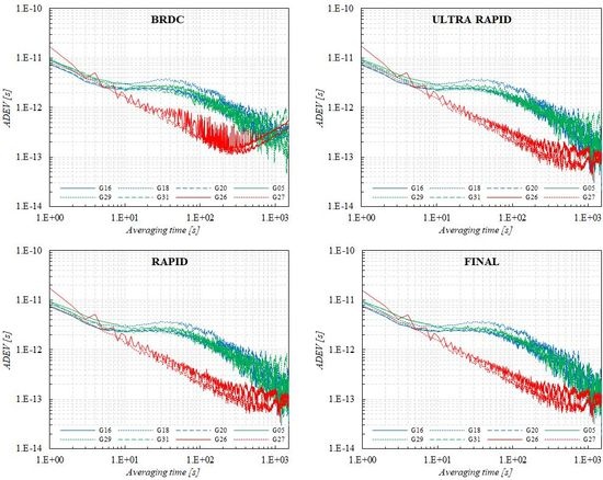
Figure 3 shows ADEV based on calculations according to two different types of orbit: broadcast and ultra-rapid. The results between three precise orbits were negligibly small, therefore the authors in the following part of this paper focused only on the navigation orbit (broadcast) and ultra-rapid (precise orbit available in real time). The ONS1 station clock was applied as a reference one for each solution. In each part of Figure 3 the most stable are the pair of satellites 26 and 27 (SVN 66 and 71), which highlights the advantage of Block IIF’s (red lines) stability in comparison to Blocks IIR (blue) and IIR-M (green). For a G26 satellite, the error bars are calculated that represent standard deviation with a 95% confidence interval. Depending on the averaging time and orbit type adopted for modelling error, the magnitudes are different. In general, a longer averaging time is affected by a larger error due to the smaller number of samples. However, a comparison of broadcast and ultra-rapid orbit dependent results shows a smaller error for a precise one orbit for each analysed averaging time. Moreover, there are no error bars on the figures presenting many τ method due to relatively much greater number of results using the 2n method (Figure 3 and Figure 4 below).
The stabilities of Blocks IIR (blue line) and IIR-M (green line) are very similar. A comparison of the orbit types between them does not show any significant differences. Table 5 presents the ADEV of the selected intervals for two analysed orbit types.
For τ = 1 and 4 s, the frequency stabilities are close to 1 × 10⁻¹² s; for τ = 16 and 64 s, every stability is close to 1 × 10⁻¹³ s; and for bigger averaging intervals stabilities—close to even 7–8 × 10⁻¹⁴ s.
4.2. Allan Deviation: All τ Method
An all τ analysis, demanding superior computational power than standard intervals, is usually applied as a consecutive power of 2, or multiplies of selected numbers. However, this method shows a wider spectrum of oscillator deviations in other than successive powers of the number 2, or other rigidly determined numbers and their multiples.
The many τ (averaging times) method shows similar results to the τ = 2n method, however a greater noise appears, especially for the higher averaging time values. The clock corrections based on precise orbits are slightly more accurate than those based on broadcast ones. Frequency stabilities generally agree with each other for both the 2n and many τ method, except for PRNs 26 and 27 (Block IIF). Analysis of the 2n and τ method graphs (Figure 3) show a very high consistency for all the averaging times between 1 and 256 s included, except for PRN18, which is less stable between 32 s to 128 s averaging times. The reason of the PRN18 stability degradation is not clear at present. For the two highest averaging times, the results are very random; in addition, they are not correlated with the satellite block type. A comparison of the analysed blocks shows almost identical stabilities for Blocks IIR and IIR-M (except for slightly worse results for PRN18). The Block IIF oscillators are slightly more stable than the other two blocks. In the case of the satellite orbit used for the calculations, there are no significant differences, excepting PRN 26 and 27 for the longest 1024 s τ on the basis of BRDC (GPS broadcast ephemeris file) calculations (Figure 3 and Figure 4, top left). Figure 4 presents ADEV calculated using consecutive (with 1 s step) averaging times beginning from 1. This approach is aimed at detecting a possible clock anomaly that was not detected by the 2n averaging times. If detected, it might have been responsible for smoothing the results. The most visible is the PRN26 oscillator stability graph using the broadcast orbit (Figure 4, top left), which is jagged compared to the other graphs, but in Figure 3 the same phenomena is also visible for this satellite only.
4.3. Time Deviation: τ = 2n
Figure 5 presents TDEV of clock products based on the broadcast and ultra-rapid orbits together with the error bars for a G26 satellites. TDEV varies between 3.9 × 10⁻¹² s to 2.9 × 10⁻¹⁰ s for broadcast orbit and between 4.0 × 10⁻¹² s to 1.9 × 10⁻¹⁰ s in case of ultra-rapid one. Analysis shows a similar behavior for a IIR and IIR-M GPS satellites, while IIF satellites (G26 and G27) are characterized by lower stability for the shortest intervals (1 s and 2 s), clearly higher for longer intervals (4–128 s), while for the highest intervals the stability of TDEV is the same. The same can be observed in the case of uncertainty estimates, error bars of results acquired by using broadcast orbit are much bigger than using ultra rapid ones.
4.4. Time Deviation: All τ Method
TDEV values of broadcast and ultra-rapid orbit using the many τ method are visible in Figure 6. The use of the many τ method shows the same results and conclusions as described in Section 4.3. Compared to Figure 4, there are no significant fluctuations in stability between successive intervals; this is due to the fact that TDEV is based on modification of the ADEV. Otherwise, TDEV presents time stability of phase versus observation interval.
5. Conclusions
The novelty of this work compared with other studies and the current state of knowledge results from three elements: an analysis of the orbit type impact on satellite clock stability, the usage of the Allan’s variance all τ method for this type of elaboration, and the high sampling frequency on the basis of 1 s observation data on the IGS stations. The main purpose of the study presented was the determination of the effect of the orbit type used on the stability of GPS clocks. Calculations in BSW on the basis of three precise orbits (ultra-rapid, rapid, and final) show very similar results, thus precise orbits available in less time (ultra-rapid in real time, rapid after 17–41 h) than the final one (after 10–18 days) can be used to analyse clock stability. Unlike in precise positioning, where final orbit is used, ultra-rapid or rapid orbit might be used without loss of results quality for this kind of elaboration. Moreover, in this paper so-called all τ method was use, unlike in all the other similar publications. In this paper, apart from the most widely used averaging times as a consecutive powers of 2 (20 s = 1 s, 21 s = 2 s, 22 = 4 s, etc.) or 10 (100 s = 1 s, 101 s = 10 s, 102 s = 100 s, etc.) or 30/300 s (based on existing clock products), the authors adopted 1 s data. The third element supporting the novelty of this paper compared to existing research is the fact of using clock corrections based on modelling using BSW software with 1 Hz observation frequency. In a future work, the authors plan to analyse clock corrections with higher frequencies than 1 Hz, up to 20 Hz.
An analysis of high-rate 1 Hz satellite clock correction is presented in this paper. IGS’s analysis centres provide rapid and final clock products with 5 s and 30 s correction intervals. For precise elaborations such as PPP, seismology or high-rate GNSS monitoring, 1 s interval clock corrections are required. In this paper, the authors show 1 s elaboration of satellite and stations clock corrections depending on the adopted orbit type and the method of ADEV and TDEV averaging time used. The emphasis has been put on the GPS satellites clock’s stability depending on the type of orbit used. The use of GPS-only signals results from the fact that the adopted software does not allow for the use of BeiDou, Galileo, and QZSS signals in this type of analysis. Currently, Bernese GNSS Software gives the opportunity to compute only GPS and GLONASS (Russian: ГЛОНАСС - Глобальная навигационная спутниковая система, transliteration: Globalnaya navigatsionnaya sputnikovaya sistema) satellite clock corrections. Moreover, this work should be treated as preliminary research in the field of determining the impact of the orbit type in the satellite clock stability analysis. The next part of the research will include analysis using GNSS signals (GPS GLONASS) and, in the future, using all currently available satellite signals (GPS, GLONASS, Galileo, BeiDou, and QZSS).
Four different orbit types were analysed: three precise with 15 min sampling intervals, and broadcast ephemeris with a 30 min sampling interval. The results from the data indicate GPS satellites frequency stability (ADEV) at a level of 1.7 × 10⁻¹¹ s to 7.2 × 10⁻¹⁴ s and time stability (TDEV) at a level of 2.9 × 10¹⁰ s to 3.9 × 10¹² s. The results also show the insignificant advantage of the satellite Block IIF’s frequency and time stabilities in regard to the other two blocks. As used in this article, the many τ method allows for detection of the satellite clock anomaly. This method might also assist in preventing the use of a satellite clock with identified potential instability patterns as a reference clock.
Author Contributions
Conceptualisation, K.M., P.L.; methodology, K.M., P.L.; software, K.M.; validation, K.M., P.L.; formal analysis, K.M., P.L.; investigation, K.M., P.L.; resources, K.M., P.L.; writing—original draft preparation, K.M., P.L.; writing—review and editing, K.M., P.L.; visualisation, P.L.; supervision, K.M., P.L.; project administration, K.M., P.L.
Funding
This paper was made within statutory research 16.16.150.545.
Conflicts of Interest
The authors declare no conflict of interest.
References
- Hordyniec, P.; Kapłon, J.; Rohm, W.; Kryza, M. Residuals of Tropospheric Delays from GNSS Data and Ray-Tracing as a Potential Indicator of Rain and Clouds. Remote Sens. 2018, 10, 1917. [Google Scholar] [CrossRef]
- Wielgosz, P.; Paziewski, J.; Baryła, R. On Constraining Zenith Tropospheric Delays in Processing of Local GPS Networks with Bernese Software. Surv. Rev. 2011, 43, 472–483. [Google Scholar] [CrossRef]
- Xie, X.; Geng, T.; Zhao, Q.; Liu, J.; Wang, B. Performance of BDS-3: Measurement Quality Analysis, Precise Orbit and Clock Determination. Sensors 2017, 17, 1233. [Google Scholar] [CrossRef]
- Yu, X.; Gao, J. Kinematic Precise Point Positioning Using Multi-Constellation Global Navigation Satellite System (GNSS) Observations. ISPRS Int. J. Geo-Inf. 2017, 6, 6. [Google Scholar] [CrossRef]
- Kaloop, M.; Elbeltagi, E.; Hu, J.; Elrefai, A. Recent Advances of Structures Monitoring and Evaluation Using GPS-Time Series Monitoring Systems: A Review. ISPRS Int. J. Geo-Inf. 2017, 6, 382. [Google Scholar] [CrossRef]
- Lv, Y.; Dai, Z.; Zhao, Q.; Yang, S.; Zhou, J.; Liu, J. Improved Short-Term Clock Prediction Method for Real-Time Positioning. Sensors 2017, 17, 1308. [Google Scholar] [CrossRef] [PubMed]
- Shi, J.; Wang, G.; Han, X.; Guo, J. Impacts of satellite orbit and clock on real-time GPS point and relative positioning. Sensors 2017, 17, 1363. [Google Scholar] [CrossRef] [PubMed]
- Gruszczynski, W. Influence of model parameter uncerainties on forecasted subsidence. Acta Geodyn. Geomater. 2018, 15, 211–228. [Google Scholar] [CrossRef]
- Niedojadło, Z.; Gruszczyński, W. The Impact of the Estimation of the Parameters Values on the Accuracy of Predicting the Impacts of Mining Exploitation/Wpływ Oszacowania Wartości Parametrów Modelu Na Dokładność Prognozowania Wpływów Eksploatacji Górniczej. Arch. Min. Sci. 2015, 60, 173–193. [Google Scholar] [CrossRef]
- Malinowska, A.A.; Hejmanowski, R.; Witkowski, W.T.; Guzy, A. Mapping of slow vertical ground movement caused by salt cavern convergence with sentinel-1 tops data. Arch. Min. Sci. 2018, 63, 383–396. [Google Scholar]
- Kampczyk, A. Geodäsie im Investitionsbauprozess auf den Bahngebieten in Polen. Bautechnik 2014, 91, 409–413. [Google Scholar] [CrossRef]
- Kampczyk, A. Technische Spezifikationen für die Interoperabilität und die polnischen Vorschriften in der Projektierung von der Geometrie der Eisenbahnstrecken/Technical specifications for interoperability and Polish regulations in the design of the geometry of railway lines. Bauingenieur 2015, 90, 229–234. [Google Scholar]
- Borowski, L.; Pienko, M.; Wielgos, P. Evaluation of Inventory Surveying of Façade Scaffolding Conducted during ORKWIZ Project. In Proceedings of the 2017 Baltic Geodetic Congress (BGC Geomatics), Gdansk, Poland, 22–25 June 2017; pp. 189–192. [Google Scholar]
- Chrobak, T.; Lupa, M.; Szombara, S.; Dejniak, D. The use of cartographic control points in the harmonization and revision of MRDBs. GEOCARTO Int. 2019, 34, 260–275. [Google Scholar] [CrossRef]
- Ligas, M.; Szombara, S. Geostatistical prediction of a local geometric geoid-kriging and cokriging with the use of EGM2008 geopotential model. Stud. Geophys. Geod. 2018, 62, 187–205. [Google Scholar] [CrossRef]
- Grešlová, P.; Štych, P.; Salata, T.; Hernik, J.; Knížková, I.; Bičík, I.; Jeleček, L.; Prus, B.; Noszczyk, T. Agroecosystem energy metabolism in Czechia and Poland in the two decades after the fall of communism: From a centrally planned system to market oriented mode of production. Land Use Policy 2019, 82, 807–820. [Google Scholar] [CrossRef]
- Bieda, A.; Bieda, A. Renewable energy in the system of spatial planning in Poland. In Proceedings of the Geographic Information Systems Conference and Exhibition (GIS ODYSSEY 2017), Trento, Italy, 4–8 September 2017; pp. 28–42. [Google Scholar]
- Bieda, A.; Adamczyk, T.; Bieda, A. The energy performance of buildings directive as one of the solutions for smart cities. In Proceedings of the Geographic Information Systems Conference and Exhibition—GIS ODYSSEY 2016, Perugia, Italy, 5–9 September 2016; pp. 44–49. [Google Scholar]
- Kukulska-Kozieł, A.; Szylar, M.; Cegielska, K.; Noszczyk, T.; Hernik, J.; Gawroński, K.; Dixon-Gough, R.; Jombach, S.; Valánszki, I.; Kovács, K.F. Towards three decades of spatial development transformation in two contrasting post-Soviet cities—Kraków and Budapest. Land Use Policy 2019, 85, 328–339. [Google Scholar] [CrossRef]
- Hanus, P.; Pęska-Siwik, A.; Szewczyk, R. Spatial analysis of the accuracy of the cadastral parcel boundaries. Comput. Electron. Agric. 2018, 144, 9–15. [Google Scholar] [CrossRef]
- Benduch, P.; Pęska-Siwik, A. Assessing the usefulness of the photogrammetric method in the process of capturing data on parcel boundaries. Geod. Cartogr. 2017, 66, 3–22. [Google Scholar] [CrossRef]
- Busko, M.; Szafranska, B. Analysis of Changes in Land Use Patterns Pursuant to the Conversion of Agricultural Land to Non-Agricultural Use in the Context of the Sustainable Development of the Malopolska Region. Sustainability 2018, 10, 136. [Google Scholar] [CrossRef]
- Busko, M.; Meusz, A. Current status of real estate cadastre in Poland with reference to historical conditions of different regions of the country. In Proceedings of the 9th International Conference Environmental Engineering (9th ICEE)—Selected Papers, Vilnius, Lithuania, 22–23 May 2014. [Google Scholar]
- Noszczyk, T. Land Use Change Monitoring as a Task of Local Government Administration in Poland. J. Ecol. Eng. 2018, 19, 170–176. [Google Scholar] [CrossRef]
- Zumberge, J.; Heflin, M.; Jefferson, D.; Watkins, M.M.; Webb, F. Precise point positioning for the efficient and robust analysis of GPS data from large networks. J. Geophys. Res. Solid Earth 1997, 102, 5005–5017. [Google Scholar] [CrossRef]
- Choy, S.; Bisnath, S.; Rizos, C. Uncovering common misconceptions in GNSS Precise Point Positioning and its future prospect. GPS Solut. 2016, 21, 1–10. [Google Scholar] [CrossRef]
- Chan, F.C.; Joerger, M.; Pervan, B. Stochastic modeling of atomic receiver clock for high integrity GPS navigation. IEEE Trans. Aerosp. Electron. Syst. 2014, 50, 1749–1764. [Google Scholar] [CrossRef]
- Wang, D.; Guo, R.; Xiao, S.; Xin, J.; Tang, T.; Yuan, Y. Atomic clock performance and combined clock error prediction for the new generation of BeiDou navigation satellites. Adv. Space Res. 2018, 63, 2889–2898. [Google Scholar] [CrossRef]
- Bock, H.; Dach, R.; Jäggi, A.; Beutler, G. High-rate GPS clock corrections from CODE: Support of 1 Hz applications. J. Geod. 2009, 83, 1083–1094. [Google Scholar] [CrossRef]
- Dach, R.; Walser, P. Bernese GNSS Software Version 5.2; Astronomical Institute, University of Bern: Bern, Switzerland, 2013. [Google Scholar]
- Cernigliaro, A.; Valloreia, S.; Fantino, G.; Galleani, L.; Tavella, P. Analysis on GNSS space clocks performances. In Proceedings of the 2013 Joint European Frequency and Time Forum & International Frequency Control Symposium (EFTF/IFC), Prague, Czech Republic, 21–25 July 2013; pp. 835–837. [Google Scholar]
- Zhang, B.; Ou, J.; Yuan, Y.; Zhong, S. Yaw attitude of eclipsing GPS satellites and its impact on solutions from precise point positioning. Chin. Sci. Bull. 2010, 55, 3687–3693. [Google Scholar] [CrossRef]
- Daly, P.; Kitching, I.D.; Allan, D.W.; Peppler, T.K. Frequency and time stability of GPS and GLONASS clocks. In Proceedings of the 44th Annual Symposium on Frequency Control, Baltimore, MD, USA, 23–25 May 1990; Volume 9, pp. 127–139. [Google Scholar]
- Delporte, J.; Boulanger, C.; Mercier, F. Short-term stability of GNSS on-board clocks using the polynomial method. In Proceedings of the 2012 European Frequency and Time Forum, Gothenburg, Sweden, 23–27 April 2012; pp. 117–121. [Google Scholar]
- Delporte, J.; Boulanger, C.; Mercier, F. Straightforward estimations of GNSS on-board clocks. In Proceedings of the 2011 Joint Conference of the IEEE International Frequency Control and the European Frequency and Time Forum (FCS) Proceedings, San Francisco, CA, USA, 2–5 May 2011; pp. 1–4. [Google Scholar]
- Qing, Y.; Lou, Y.; Dai, X.; Liu, Y. Benefits of satellite clock modeling in BDS and Galileo orbit determination. Adv. Space Res. 2017, 60, 2550–2560. [Google Scholar] [CrossRef]
- Lee, S.W.; Kim, J.; Lee, Y.J. Protecting signal integrity against atomic clock anomalies on board GNSS satellites. IEEE Trans. Instrum. Meas. 2011, 60, 2738–2745. [Google Scholar] [CrossRef]
- Maciuk, K. Satellite clock stability analysis depending on the reference clock type. Arab. J. Geosci. 2019, 12, 28. [Google Scholar] [CrossRef]
- Maciuk, K. Monitoring of Galileo on-board oscillators variations, disturbances & noises. Measurement 2019, 147, 106843. [Google Scholar]
- Wang, S.; Yang, F.; Gao, W.; Yan, L.; Ge, Y. A new stochastic model considering satellite clock interpolation errors in precise point positioning. Adv. Space Res. 2018, 61, 1332–1341. [Google Scholar] [CrossRef]
- Guo, F.; Zhang, X.; Li, X.; Cai, S. Impact of sampling rate of IGS satellite clock on precise point positioning. Geo-Spat. Inf. Sci. 2010, 13, 150–156. [Google Scholar] [CrossRef]
- Yeh, T.-K.; Hwang, C.; Xu, G.; Wang, C.-S.; Lee, C.-C. Determination of global positioning system (GPS) receiver clock errors: Impact on positioning accuracy. Meas. Sci. Technol. 2009, 20, 075105. [Google Scholar] [CrossRef]
- Elsobeiey, M.; Al-Harbi, S. Performance of real-time Precise Point Positioning using IGS real-time service. GPS Solut. 2016, 20, 565–571. [Google Scholar] [CrossRef]
- Lutz, S.; Beutler, G.; Schaer, S.; Dach, R.; Jäggi, A. CODE’s new ultra-rapid orbit and ERP products for the IGS. GPS Solut. 2016, 20, 239–250. [Google Scholar] [CrossRef] [Green Version]
- Luo, X. Mathematical Models for GPS Positioning. In GPS Stochastic Modelling; Springer: Berlin/Heidelberg, Germany, 2013; pp. 55–116. [Google Scholar]
- Fu, W.; Huang, G.; Liu, Y.; Zhang, Q.; Yu, H. The analysis of the characterization for GLONASS and GPS on-board satellite clocks. Lect. Notes Electr. Eng. 2013, 244, 549–566. [Google Scholar]
- Leick, A.; Rapoport, L.; Tatarnikov, D. GPS Satellite Surveying, 4th ed.; John Wiley & Sons, Inc.: Hoboken, NJ, USA, 2015. [Google Scholar]
- ICD-GPS-870. NAVSTAR GPS Interface Control Document. 2017. Available online: https://www.gps.gov/technical/icwg/ (accessed on 25 October 2019).
- Petovello, M.G.; Lachapelle, G. Estimation of Clock Stability Using GPS. GPS Solut. 2000, 4, 21–33. [Google Scholar] [CrossRef]
- Allan, D.W. Clock characterization tutorial. In Proceedings of the 15th Annual Precise Time and Time Interval (PTTI) Applications and Planning Meeting, Washington, DC, USA, 6–8 December 1983; pp. 459–475. [Google Scholar]
- Allan, D.W. Time and Frequency (Time-Domain) Characterization, Estimation, and Prediction of Precision Clocks and Oscillators. IEEE Trans. Ultrason. Ferroelectr. Freq. Control 1987, 34, 647–654. Available online: https://tf.nist.gov/general/pdf/2082.pdf (accessed on 25 October 2019). [CrossRef]
- Riley, W.J. Handbook of Frequency Stability Analysis; National Institute of Standards and Technology: Washington, DC, USA, 2008. [Google Scholar]
- Allan, D.W.; Weiss, M.A.; Jespersen, J.L. A frequency-domain view of time-domain characterization of clocks and time and frequency distribution systems. In Proceedings of the 45th Annual Symposium on Frequency Control 1991, Los Angeles, CA, USA, 29–31 May 1991; pp. 667–678. [Google Scholar]
- Zhang, X.; Li, X.; Guo, F. Satellite clock estimation at 1 Hz for realtime kinematic PPP applications. GPS Solut. 2011, 15, 315–324. [Google Scholar] [CrossRef]
- Han, S.-C.; Kwon, J.H.; Jekeli, C. Accurate absolute GPS positioning through satellite clock error estimation. J. Geod. 2001, 75, 33–43. [Google Scholar] [CrossRef]
- Delporte, J. Simple methods for the estimation of the short-term stability of GNSS on-board clocks. In Proceedings of the 42nd Annual Precise Time and Time Interval Applications Planning Meeting, Reston, VA, USA, 15–18 November 2010; pp. 215–223. [Google Scholar]
Figure 1.
Distribution of the 14 stations involved in the experiment (generated by http://www.simplemappr.net/).
Figure 1.
Distribution of the 14 stations involved in the experiment (generated by http://www.simplemappr.net/).
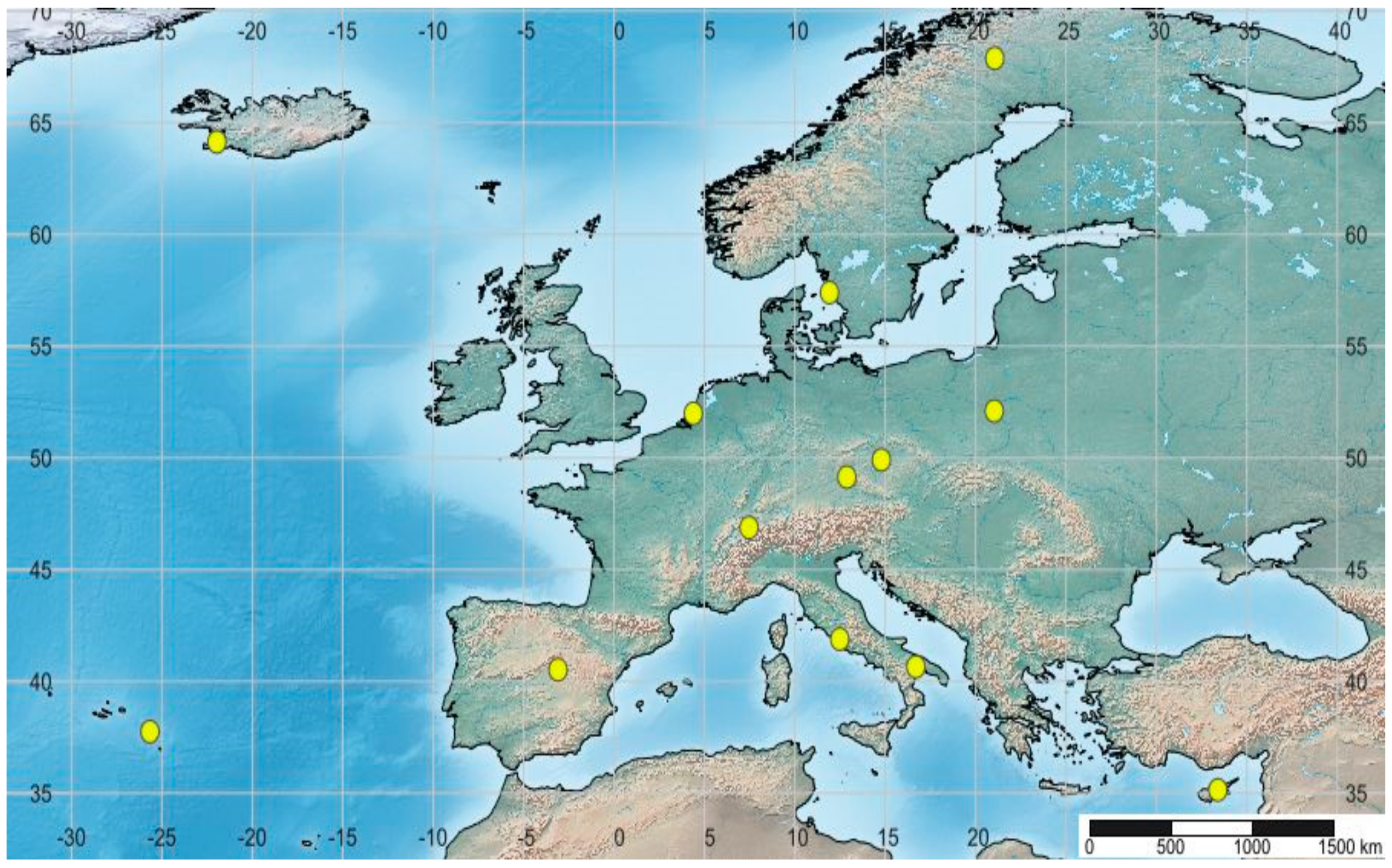
Figure 2.
Allan deviation (ADEV) of H-maser oscillators in the analysed network.
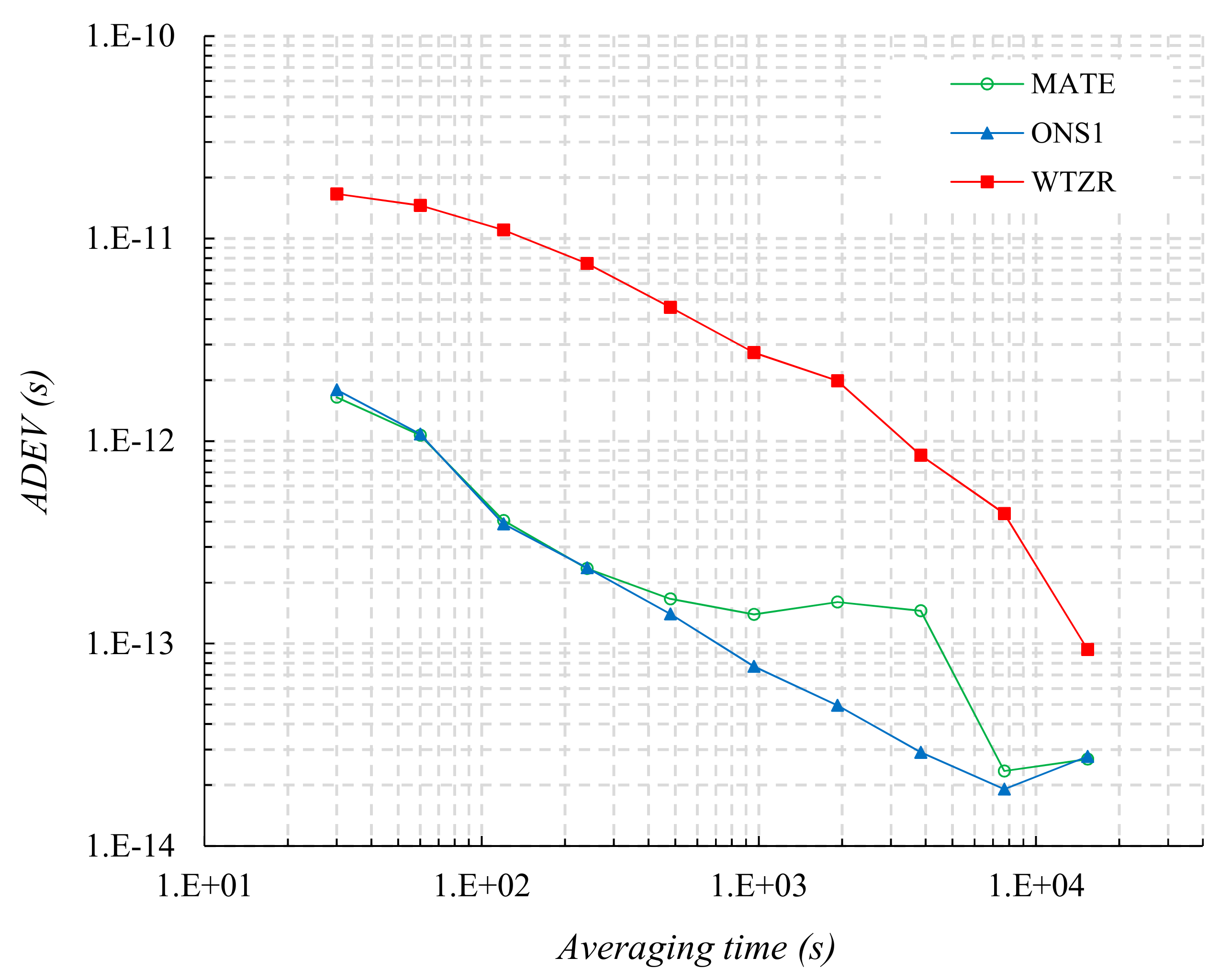
Figure 3.
ADEV depending on orbit type using τ = 2n.
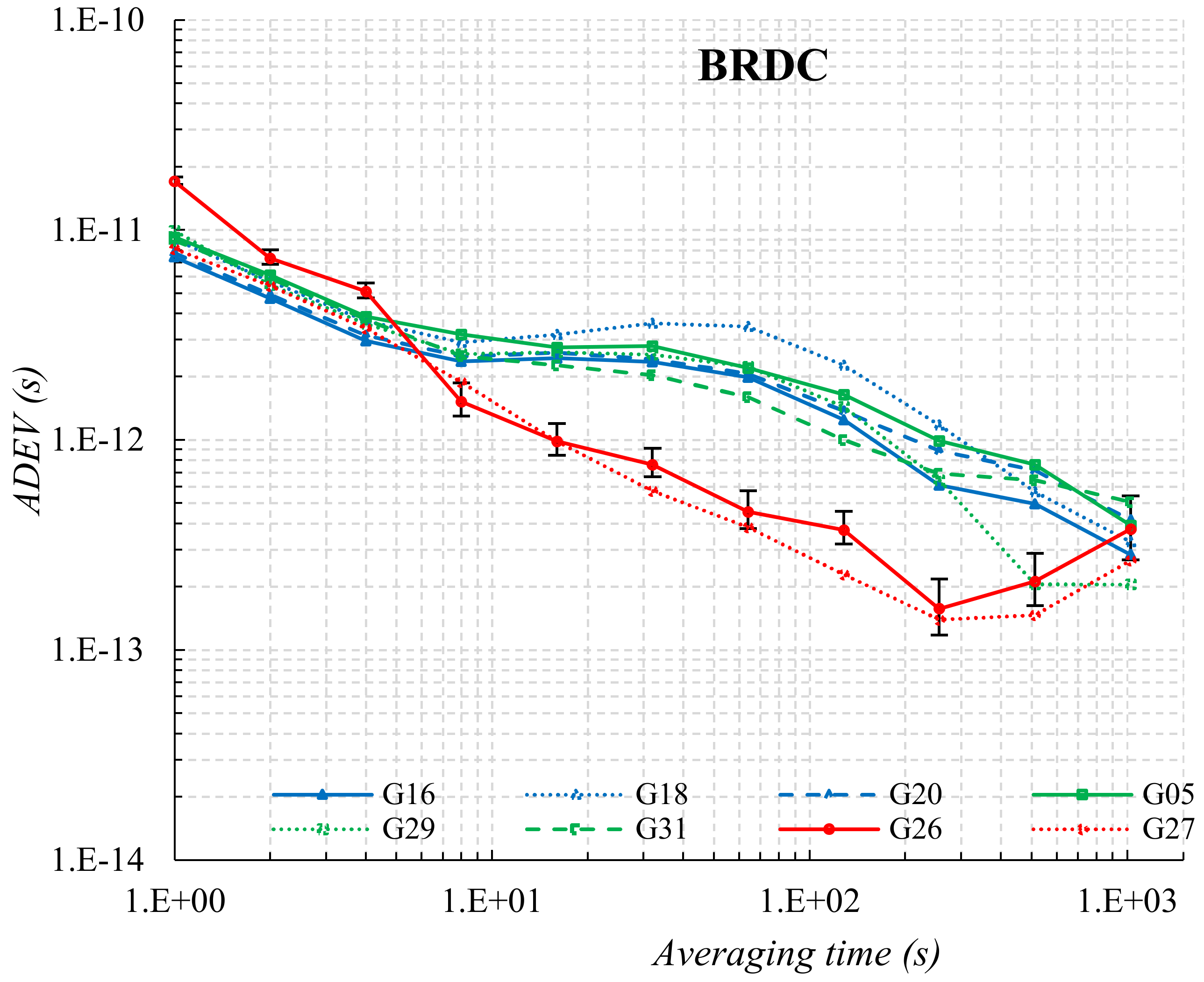

Figure 4.
ADEV depending on orbit type using the many τ method.
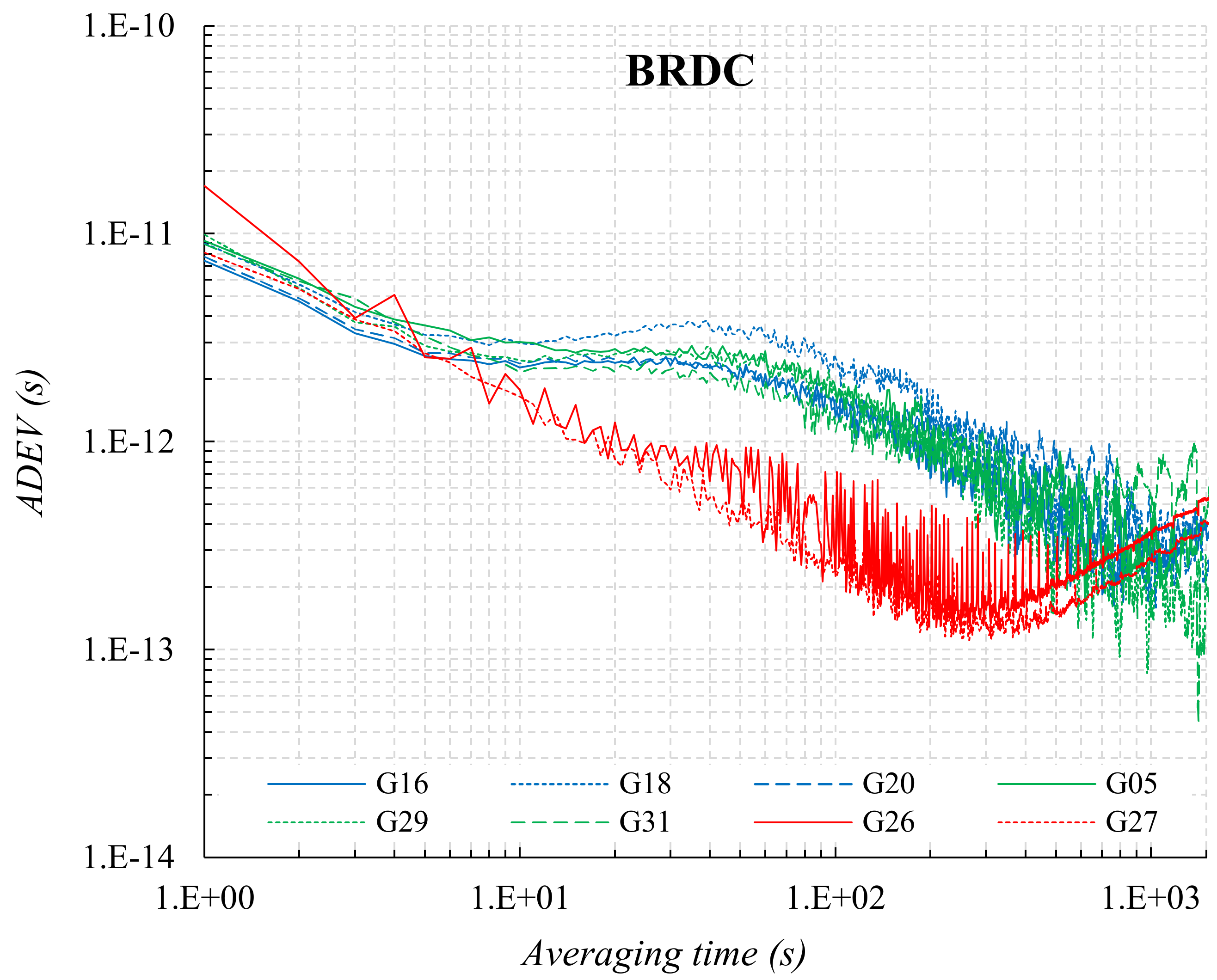
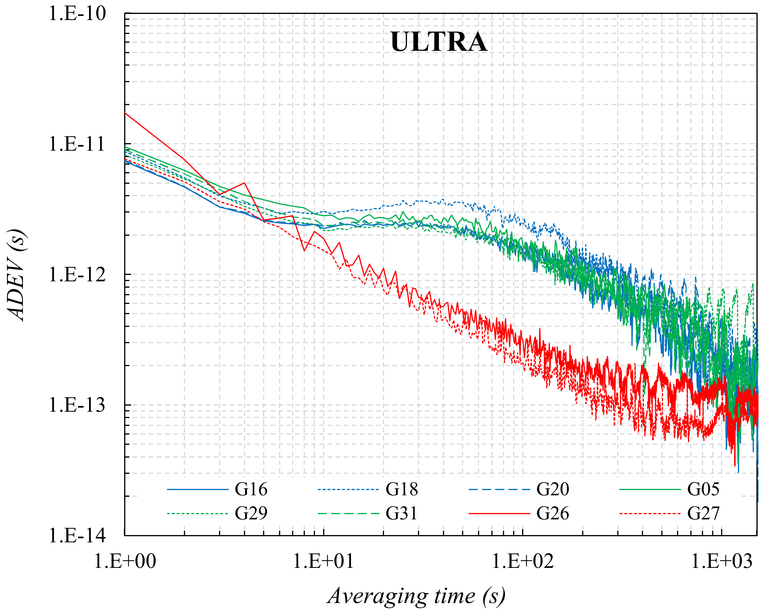
Figure 5.
Time Allan variance (TVAR), with square root (TDEV) depending on orbit type using τ = 2n.
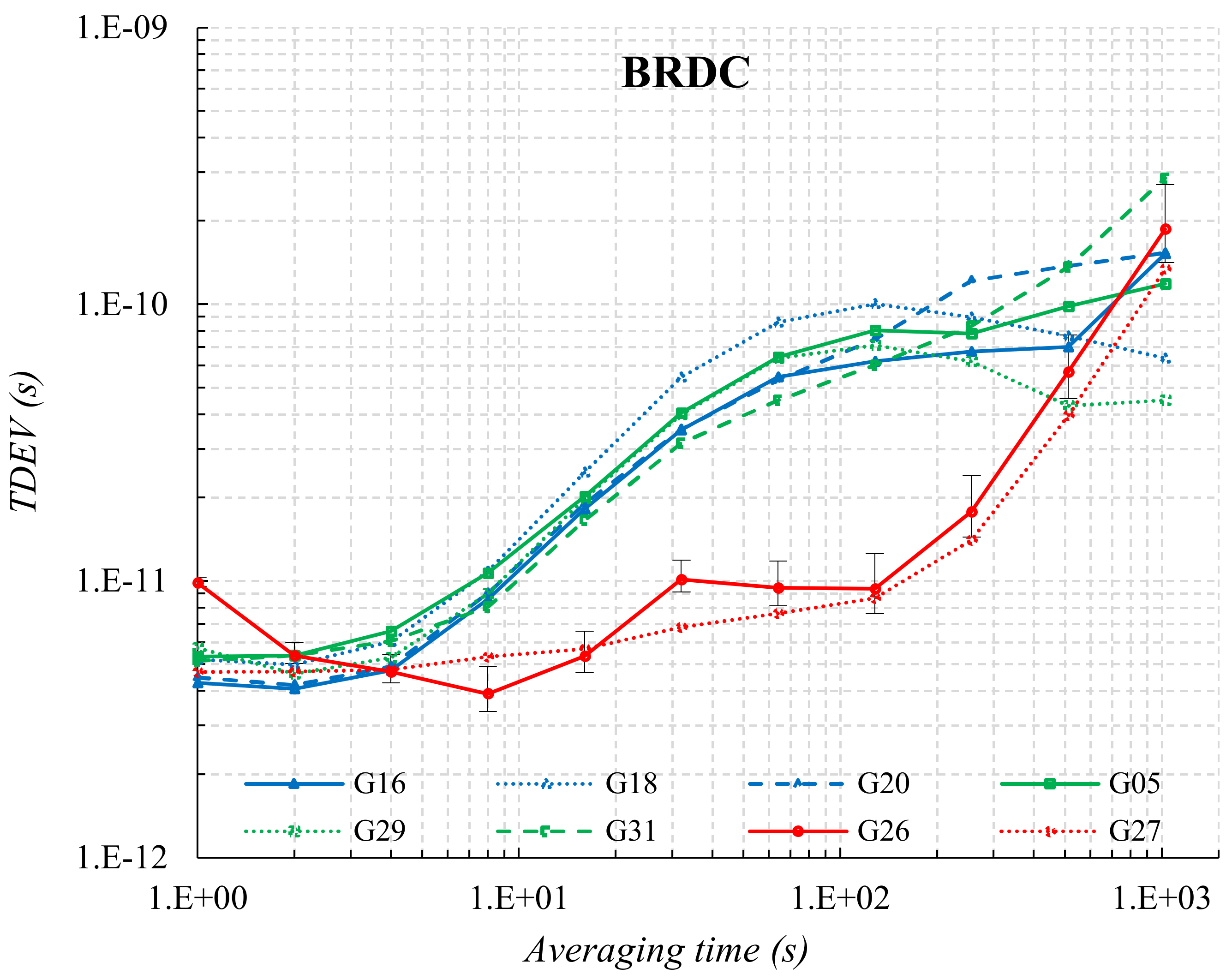

Figure 6.
ADEV depending on orbit type using the many τ method.


Table 1.
GPS satellite ephemeris, satellite and station clocks (http://www.igs.org/products).
Table 1.
GPS satellite ephemeris, satellite and station clocks (http://www.igs.org/products).
| Type | Accuracy | Latency | Updates (Per Day) |
|---|---|---|---|
| Broadcast | ~100 cm | real time | 12 |
| ~5 ns | |||
| Ultra-Rapid (predicted half) | ~5 cm | real time | 4 |
| ~3 ns | |||
| Ultra-Rapid (observed half) | ~3 cm | 3–9 h | 4 |
| ~150 ps | |||
| Rapid | ~2.5 cm | 17–41 h | 1 |
| ~75 ps | |||
| Final | ~2.5 cm | 12–18 days | 1 week |
Table 2.
Selected characteristic features of the different global positioning system (GPS) satellite categories [45].
Table 2.
Selected characteristic features of the different global positioning system (GPS) satellite categories [45].
| Satellite Category | Launches During | SVN a | Atomic Clock | Design Life (Years) |
|---|---|---|---|---|
| Block I | 1978–1985 | 01–11 (07) b | 1 Cs + 2 Rb | 4.5 |
| Block II | 1989–1990 | 13–21 | 2 Cs + 2 Rb | 7.5 |
| Block IIA | 1990–1997 | 22–40 | 2 Cs + 2 Rb | 7.5 |
| Block IIR | 1997–2004 | 41–61 (42) | 3 Rb | 10 |
| Block IIR-M | 2005–2009 | 48–58 | 3 Rb | 10 |
| Block IIF | 2010–2012 | 62–73 | 1 Cs + 2 Rb | 12.7 |
a satellite vehicle number b unsuccessful launches provided in brackets.
Table 3.
Tracking stations involved in the experiment.
| Station | Country | City | Clock |
|---|---|---|---|
| DLF1 | Netherlands | Delft | External Caesium |
| GOP6 | Czech Republic | Ondrejov | External Caesium |
| GOP7 | Czech Republic | Ondrejov | External Caesium |
| JOZ2 | Poland | Jozefoslaw | Internal |
| KIR8 | Sweden | Kiruna | External Rubidium |
| M0SE | Italy | Rome | External Rubidium |
| MATE | Italy | Matera | External H_Maser |
| NICO | Cyprus | Nicosia | Internal |
| ONS1 | Sweden | Onsala | External H-Maser |
| PDEL | Portugal | Ponta Delgada | External Quartz |
| REYK | Iceland | Reykjavik | Internal |
| WTZR | Germany | Bad Koetzting | External H-Maser |
| YEBE | Spain | Yebes | External H-Maser |
| ZIM2 | Switzerland | Zimmerwald | Internal |
Table 4.
Information about the satellites used in the experiment (http://www2.unb.ca/gge/Resources/GPSConstellationStatus.txt, https://www.navcen.uscg.gov/?Do=constellationstatus).
Table 4.
Information about the satellites used in the experiment (http://www2.unb.ca/gge/Resources/GPSConstellationStatus.txt, https://www.navcen.uscg.gov/?Do=constellationstatus).
| PRN a | SVN | Orbit Plane | Block | Freq. Standard | Launch Date | Available (UT) |
|---|---|---|---|---|---|---|
| G20 | 51 | E4 | IIR-4 | Rb1 | 2000-05-11 | 2000-06-01 16:09 |
| G18 | 34 | D6 | IIR-7 | Rb1 | 2001-01-30 | 2001-02-15 15:51 |
| G16 | 56 | B1 | IIR-8 | Rb3 | 2003-01-29 | 2003-02-18 15:53 |
| G31 | 52 | A2 | IIR-M-2 | Rb3 | 2006-09-25 | 2006-10-12 22:53 |
| G29 | 57 | C1 | IIR-M-5 | Rb3 | 2007-12-20 | 2008-01-02 20:41 |
| G05 | 50 | E3 | IIR-M-8 | Rb1 | 2009-08-17 | 2009-08-27 14:40 |
| G27 | 66 | C2 | IIF-4 | Rb2 | 2013-05-15 | 2013-06-21 19:58 |
| G26 | 71 | B5 | IIF-9 | Rb1 | 2015-03-25 | 2015-04-20 22:22 |
a Pseudo Random Noise.
Table 5.
Allan deviation of selected 2n intervals.
| Orbit Type | PRN | τ [s] | |||||
|---|---|---|---|---|---|---|---|
| 1 | 4 | 16 | 64 | 256 | 1024 | ||
| Broadcast | G16 | 7.42 × 10⁻¹² | 2.95 × 10⁻¹² | 2.44 × 10⁻¹² | 1.98 × 10⁻¹² | 6.08 × 10⁻¹³ | 2.85 × 10⁻¹³ |
| G20 | 7.77 × 10⁻¹² | 3.15 × 10⁻¹² | 2.61 × 10⁻¹² | 2.07 × 10⁻¹² | 8.89 × 10⁻¹³ | 4.16 × 10⁻¹³ | |
| G27 | 8.12 × 10⁻¹² | 3.40 × 10⁻¹² | 9.82 × 10⁻¹³ | 3.83 × 10⁻¹³ | 1.39 × 10⁻¹³ | 2.67 × 10⁻¹³ | |
| G18 | 9.02 × 10⁻¹² | 3.68 × 10⁻¹² | 3.18 × 10⁻¹² | 3.46 × 10⁻¹² | 1.18 × 10⁻¹² | 3.27 × 10⁻¹³ | |
| G26 | 1.70 × 10⁻¹² | 5.08 × 10⁻¹² | 9.83 × 10⁻¹³ | 4.55 × 10⁻¹³ | 1.57 × 10⁻¹³ | 3.75 × 10⁻¹³ | |
| G29 | 9.90 × 10⁻¹² | 3.58 × 10⁻¹² | 2.61 × 10⁻¹² | 2.24 × 10⁻¹² | 6.45 × 10⁻¹³ | 2.05 × 10⁻¹³ | |
| G31 | 8.90 × 10⁻¹² | 3.75 × 10⁻¹² | 2.27 × 10⁻¹² | 1.60 × 10⁻¹² | 6.91 × 10⁻¹³ | 5.07 × 10⁻¹³ | |
| G05 | 9.24 × 10⁻¹² | 3.86 × 10⁻¹² | 2.76 × 10⁻¹² | 2.20 × 10⁻¹² | 9.91 × 10⁻¹³ | 3.92 × 10⁻¹³ | |
| Ultra-Rapid | G16 | 7.36 × 10⁻¹² | 2.94 × 10⁻¹² | 2.43 × 10⁻¹² | 1.99 × 10⁻¹² | 6.04 × 10⁻¹³ | 1.93 × 10⁻¹³ |
| G20 | 7.52 × 10⁻¹² | 3.01 × 10⁻¹² | 2.59 × 10⁻¹² | 2.07 × 10⁻¹² | 8.84 × 10⁻¹³ | 2.95 × 10⁻¹³ | |
| G27 | 7.67 × 10⁻¹² | 3.17 × 10⁻¹² | 8.34 × 10⁻¹³ | 3.07 × 10⁻¹³ | 1.18 × 10⁻¹³ | 8.05 × 10⁻¹³ | |
| G18 | 8.76 × 10⁻¹² | 3.51 × 10⁻¹² | 3.12 × 10⁻¹² | 3.41 × 10⁻¹² | 1.03 × 10⁻¹² | 1.88 × 10⁻¹³ | |
| G26 | 1.73 × 10⁻¹¹ | 5.01 × 10⁻¹² | 9.71 × 10⁻¹³ | 4.43 × 10⁻¹³ | 1.82 × 10⁻¹³ | 1.42 × 10⁻¹³ | |
| G29 | 8.31 × 10⁻¹² | 3.32 × 10⁻¹² | 2.31 × 10⁻¹² | 1.75 × 10⁻¹² | 7.33 × 10⁻¹³ | 7.28 × 10⁻¹³ | |
| G31 | 9.05 × 10⁻¹² | 3.61 × 10⁻¹² | 2.50 × 10⁻¹² | 1.88 × 10⁻¹² | 7.56 × 10⁻¹³ | 2.63 × 10⁻¹³ | |
| G05 | 9.49 × 10⁻¹² | 4.04 × 10⁻¹² | 2.76 × 10⁻¹² | 2.03 × 10⁻¹² | 9.72 × 10⁻¹³ | 4.22 × 10⁻¹³ | |
© 2019 by the authors. Licensee MDPI, Basel, Switzerland. This article is an open access article distributed under the terms and conditions of the Creative Commons Attribution (CC BY) license (http://creativecommons.org/licenses/by/4.0/).
Share and Cite
MDPI and ACS Style
Maciuk, K.; Lewińska, P. High-Rate Monitoring of Satellite Clocks Using Two Methods of Averaging Time. Remote Sens. 2019, 11, 2754. https://doi.org/10.3390/rs11232754
AMA Style
Maciuk K, Lewińska P. High-Rate Monitoring of Satellite Clocks Using Two Methods of Averaging Time. Remote Sensing. 2019; 11(23):2754. https://doi.org/10.3390/rs11232754
Chicago/Turabian StyleMaciuk, Kamil, and Paulina Lewińska. 2019. "High-Rate Monitoring of Satellite Clocks Using Two Methods of Averaging Time" Remote Sensing 11, no. 23: 2754. https://doi.org/10.3390/rs11232754
Note that from the first issue of 2016, this journal uses article numbers instead of page numbers. See further details here.