Article

Inter-Calibration of the OSIRIS-REx NavCams with Earth-Viewing Imagers

1
NASA Langley Research Center, Hampton, VA 23666, USA
2
Science Systems and Applications, Inc. 1 Enterprise Pkwy, Hampton, VA 23666, USA
3
NASA Goddard Space Flight Center, Greenbelt, MD 20771, USA
4
Lunar and Planetary Laboratory, University of Arizona, Tucson, AZ 85721, USA
*
Author to whom correspondence should be addressed.
Remote Sens. 2019, 11(22), 2717; https://doi.org/10.3390/rs11222717
Submission received: 21 October 2019 / Revised: 12 November 2019 / Accepted: 12 November 2019 / Published: 19 November 2019
(This article belongs to the Special Issue Remote Sensing: 10th Anniversary)

Abstract

:
The Earth-viewed images acquired by the space probe OSIRIS-REx during its Earth gravity assist flyby maneuver on 22 September 2017 provided an opportunity to radiometrically calibrate the onboard NavCam imagers. Spatially-, temporally-, and angularly-matched radiances from the Earth viewing GOES-15 and DSCOVR-EPIC imagers were used as references for deriving the calibration gain of the NavCam sensors. An optimized all-sky tropical ocean ray-matching (ATO-RM) calibration approach that accounts for the spectral band differences, navigation errors, and angular geometry differences between NavCam and the reference imagers is formulated in this paper. Prior to ray-matching, the GOES-15 and EPIC pixel level radiances were mapped into the NavCam field of view. The NavCam 1 ATO-RM gain is found to be 9.874 × 10⁻² Wm−2sr−1µm−1DN−1 with an uncertainty of 3.7%. The ATO-RM approach predicted an offset of 164, which is close to the true space DN of 170. The pre-launch NavCam 1 and 2 gains were compared with the ATO-RM gain and were found to be within 2.1% and 2.8%, respectively, suggesting that sensor performance is stable in space. The ATO-RM calibration was found to be consistent within 3.9% over a factor of ±2 NavCam 2 exposure times. This approach can easily be adapted to inter-calibrate other space probe cameras given the current constellation of geostationary imagers.

Graphical Abstract

1. Introduction

OSIRIS-REx (Origins, Spectral Interpretation, Resource Identification, and Security–Regolith Explorer) is a NASA mission designed to characterize the geology, texture, morphology, geochemistry, and spectral properties of the near-Earth asteroid (101955) Bennu [1]. Bennu is a carbonaceous asteroid thought to contain remnants of the building blocks of the solar system. Bennu has a mean radius of 246 m and orbits the sun with a semi-major axis of 1.13 astronomical unit (AU), which is situated between Earth (1.0 AU) and Mars (1.52 AU). The probe is designed to map the asteroid surface at a distance between 5 km and 0.7 km above the surface. Once the remote sensing of the asteroid is complete, the probe will return a minimum 60-g sample of pristine carbonaceous asteroid regolith for later lab analysis on Earth. The probe was launched on 8 September 2016 and reached Bennu on 3 December 2018 [2]. The probe will depart Bennu in 2021 and return to Earth to land at the Utah Test and Training Range on 24 September 2023. A more detailed overview of the mission is contained in Lauretta et al. 2017 [3].
The Touch and Go Camera System (TAGCAMS) was included in the spacecraft suite of instruments to support optical navigation during asteroid proximity operations, provide images for on-board natural feature tracking during sample acquisition, and document the asteroid sample stow operations [4]. TAGCAMS contains 3 cameras: NavCam 1, NavCam 2, and StowCam. NavCam 1 is the primary optical navigation camera during most mission phases, acquiring images of star fields and the target asteroid to determine spacecraft ephemerides. NavCam 2 is identical to NavCam 1, except that its boresight is optimized for Natural Feature Tracking (NFT) imaging. It serves as a back-up to NavCam 1 and is the primary natural feature tracking camera. StowCam is identical to NavCam 1 and NavCam 2 except that it is pointed at the Sample Return Capsule (SRC) and includes an integrated Bayer color filter on its detector and its lens is focused to provide optimal imaging of the interior of the OSIRIS-REx sample return capsule. Since there is no auto exposure capability on the cameras, the camera calibration is critical for setting exposure times when observing Bennu or other celestial bodies that are in the camera field of view. Accurately calibrated NavCam images also allow for more exact measurements of Bennu’s albedo. After arrival at Bennu, NavCam 1 imaged a series of point-source objects off the limb of the asteroid [
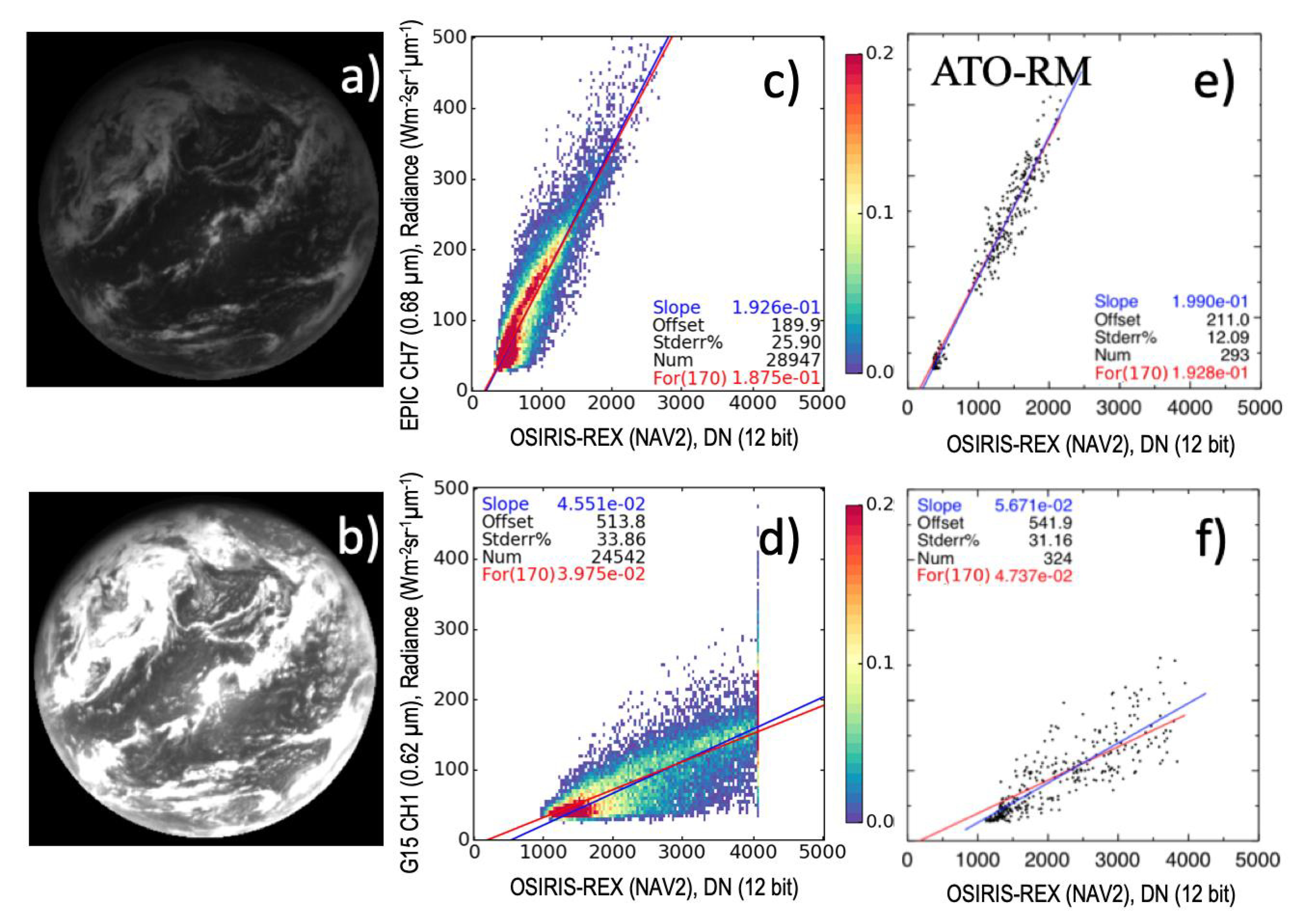
5]. Analysis of these calibrated images suggest that the objects are particles that are accelerated and ejected from the surface. To verify the camera pre-launch radiometric calibration, the spacecraft operations captured 23 NavCam 1 and three NavCam 2 images of Earth during an Earth gravity assist (EGA) flyby maneuver on 22 September 2017. These images contain the nearly-fully illuminated Earth disk centered over the East Pacific Ocean (Figure 1).
The constellation of well-calibrated Earth-viewing satellite imagers provide a calibration reference to radiometrically scale the NavCam response. The most direct inter-satellite calibration approach compares simultaneous nadir overpass (SNO) radiance pairs from two sensors [6,7]. It has now become routine to inter-calibrate operational sensor visible channels with well-calibrated sensors, such as Moderate Resolution Imaging Spectroradiometer (MODIS) and Visible Infrared Imaging Radiometer Suite (VIIRS). For example, the Advanced Very-High-Resolution Radiometer (AVHRR) sensor series [8,9,10,11,12] and the geostationary (GEO) imager [13,14,15] constellation were inter-calibrated with MODIS. Under ideal circumstances, the well-calibrated MODIS or VIIRS sensors could possibly be used to directly inter-calibrate the NavCam images. However, all of the NavCam images were sampled during a period of 1.5 h period, during which only one MODIS or VIIRS swath was available for inter-calibration.
Given the circumstances, the best NavCam inter-calibration opportunity would be with a well-calibrated GEO imager. GEO imagers are located at the equatorial latitude in an Earth-relative stationary orbit, and continuously observe the same spatial extent of Earth below. This setup allows the GEO imager to capture multiple images during the OSIRIS-REx EGA maneuver. This study calibrates the sequence of NavCam images by utilizing coincident ray-matched NavCam and GEO imager radiance pairs. The NavCam images are mostly centered over the Geostationary Operational Environmental Satellite (GOES)-15 geostationary domain, which has a subsatellite longitude of 135° West at 0° latitude. The other neighboring Himwari-8 and GOES-16 GEO imagers, which are located at 140° East and 90° West, respectively, are too far away to provide any near-nadir views of the NavCam geographic domain. Another NavCam inter-calibration prospect used in this study is the Deep Space Climate Observatory Earth Polychromatic Camera (DSCOVR-EPIC) imager [16]. The DSCOVR satellite obit is located at an Earth and sun gravitational minima or Lagrangian point (L1) and has the same sun-relative orbital period as Earth. This configuration enables the EPIC imager to continuously observe the sunlit side of Earth.
This study first radiometrically scales both the GOES-15 and DSCOVR-EPIC imager visible bands to the same Aqua-MODIS C6.1 band 1 (0.65µm) reference calibration using the NASA Clouds and the Earth’s Radiant Energy System (CERES) project GEO/MODIS all-sky tropical ocean ray-matching (ATO-RM) calibration approach [13]. The CERES ATO-RM algorithm was validated using multiple well-characterized desert targets and a deep convective cloud ray-matching (DCC-RM) algorithm, and it was found that the multiple independent calibration approaches were consistent within 1% [13]. This study modifies the ATO-RM algorithm to inter-calibrate the NavCam image response with both the GOES-15 and EPIC sensors. The greatest challenge is finding a balance between the degree of angular matching and sufficient radiance pair sampling across the dynamic range to perform a meaningful linear regression. Another challenge is the NavCam spectral band response, which is very broad compared with the GOES-15 and EPIC spectral response functions. Inadequate angle matching and spectral adjustments may bias the NavCam calibration results.
Section 2 of this paper describes the NavCam, GOES-15 and EPIC datasets. The mapping of the GOES-15 and EPIC pixel-level radiances into the NavCam field of view is discussed in Section 3. Section 4 outlines the modified NavCam ATO-RM approach that optimizes the angle matching and spectral adjustments. The ATO-RM calibration results for the two NavCam imagers are described in Section 5. Section 6 provides the best estimate of the NavCam 1 gain and uncertainty. Section 7 compares the NavCam gain with the pre-launch gain. Conclusions are provided in Section 8.

2. Data

2.1. OSIRIS-REx NavCam Data

A total of 23 NavCam 1 and three NavCam 2 Earth-view images were obtained from the OSIRIS-REx EGA data set [17]. These images were acquired for calibration purposes during the OSIRIS-REx probe EGA maneuver on 22 September 2017. The NavCam images were taken between 21:08:30 and 22:16:35 GMT, during which the probe trajectory was located between 110,500 and 137,200 km away from the surface of the Earth. Both NavCam 1 and 2 have a medium field of view of 44° by 32° and a 2592 × 1944 pixel complementary metal oxide semiconductor (CMOS) detector array [4]. The on-axis pixel scale is 0.28 mrad/pixel. This translates into a 31 km nadir pixel spatial resolution for the NavCam 1 21:08:30 GMT image and a 37 km pixel resolution for the NavCam 2 22:16:38 GMT image. Earth was not centered but, instead, was positioned over many locations across the NavCam field of view (Figure 1a). The Earth disk encompasses ~390 × 390 and ~300 × 300 pixels for the first and last NavCam images taken, respectively. The silicon detector response is limited by a piece of coated fused silica, which provides a band spectral response function having a full width at half maximum between 0.4 µm and 0.7 µm. The detector array has a digitization rate of 12 bits. The flat-fielding of the CMOS array is very good, where the edge of the image has a relative radiance decrease of 1.1% compared to the center. The camera lens introduces barrel distortion at the corners of the field of view, which was measured during in-flight star-field calibrations to be 13.9%. The NavCam on-chip gain amplifier has a commandable gain setting between 1 and 7.75. The exposure time of all the NavCam 1 images and the first NavCam 2 image is 0.1528 milliseconds, and the exposures times of the second and third NavCam 2 images are 0.0764 and 0.3228 milliseconds, respectively.

2.2. GOES-15 Data

Four GOES-15 images acquired on 22 September 2017 were downloaded from the Man computer Interactive Data Access System (McIDAS) servers [18]. This data set includes the 21:00 (identified by the start time) GMT full disk (FD) scan, which ends at 21:22 GMT at the South Pole, and three Northern Hemisphere (NH) scans that start at 21:30, 22:00, and 22:30 GMT and terminate at the Equator 12 min later (Figure 1c). The GOES-15 imager has one visible channel (centered at 0.65 µm with a bandwidth of 0.2 µm) with a nominal pixel resolution of 1 km. The visible image is constructed by an eight-pixel detector array, which scans in the east–west direction and steps north-to-south [19]. The GOES-15 data are sub-sampled at a 4 km resolution by capturing only every fourth line and element. The GOES-15 FD and NH 4 km nominal images are 2705 × 5196 and 1355 × 3312 pixels, respectively.
The CERES ATO-RM calibration approach [13,20] references the GEO imagers to the radiometric scale of the Aqua-MODIS Collection 6.1 band 1 calibration. During OSIRIS-REx’s EGA maneuver, the calibration slope of the GOES-15 imager was computed to be 0.9041 Wm−2sr−1µm−1DN−1 with a 1-σ uncertainty of 1.1% based on ATO-RM. The space offset for GOES-15 imager was 29 DN [21]. The McIDAS software also provides the pixel-level navigation and GMT time for each scan line from which the viewing and solar geometry are computed.

2.3. DSCOVR EPIC Data

The DSCOVR EPIC version 2 L1b data were obtained from the NASA-Langley Atmospheric Science Data Center Distributed Active Archive Center (ASDC DAAC) [22]. Launched on 11 February 2015, the DSCOVR satellite reached its orbit at 1.5 million km away from Earth in the solar direction on 8 June 2015. The DSCOVR satellite orbits at the sun-Earth L1 Lagrangian position, allowing the EPIC imager to view the nearly complete sunlit disk of Earth [16]. The EPIC sensor views Earth between the backscattering angles of 168.5° and 175.5°. The EPIC image is constructed from a 2048 × 2048 charge-coupled device (CCD) array of detectors having a nominal pixel resolution of 18 km (Figure 1d) [23]. The EPIC sensor uses a filter wheel to observe the sunlit side of Earth in 10 visible bands. Band 7 (center wavelength of 680 nm with a 2-nm bandwidth) is used in this study. The EPIC pixel quantization rate is 12 bits, with a per-second photon measuring frequency. Two EPIC images acquired on 22 September 2017 at 20:53 GMT and 22:41 GMT were downloaded. The EPIC version 2 L1B images are not well navigated. The true and observed pixel center latitude and longitude typically differ by an average of 50 km [24]. The EPIC navigation was accounted for in Section 3, where the EPIC image is mapped into the NavCam image.
The EPIC calibration was based on the ATO calibration approach of Doelling et al. 2019 [24], which is very similar to the CERES GOES-15/MODIS ATO-RM approach. For 22 September 2017, the EPIC pixel level DN gain, gain uncertainty, and space offset DN were estimated to be 4.769 × 10⁻³ Wm−2sr−1µm−1(DN/sec)−1, 0.6%, and 0, respectively. The EPIC dataset provides the pixel-level navigation and angular geometry.

3. NavCam Image Navigation and Mapping Methodology

Prior to ray-matching, the GOES-15 or EPIC pixel level radiances have to be collocated with NavCam CMOS pixels. Instead of mapping each of the datasets to a pre-selected geographic projection it was decided to map higher-resolution data (GOES-15 and EPIC) directly into the lower-resolution domain of NavCam image coordinates. This allows the NavCam pixels to retain their original DN thereby reducing errors caused by resampling. Another reason for this decision is the fact that any potential spatial mismatch between the two datasets should be attributed to the unknown alignment of the NavCam images, which in turn is easier to correct for when working within the NavCam image coordinates.
At the time of this study the only verified navigation information about the NavCam imager was the (x,y,z)-coordinates of OSIRIS-REx platform location in space and the tilt angle between the camera’s vertical axis and Earth’s rotational axis. We can define the camera’s coordinate frame with z-axis pointing from the satellite to Earth’s center, y-axis aligned with the apparent Earth’s rotational axis (as viewed by the camera), and x-axis complements the yz-axes to form a right-handed coordinate system. The view vector (0,0,1) pointing from the satellite to Earth’s center can easily be transformed into the Earth-centered rotational (ECR) coordinate frame, which gives us the geolocation for a pixel in the center of the apparent Earth disk. Any other view vector corresponding to a pixel within the Earth disk can be described by two angles, yaw and pitch, defined as deviations from the (0,0,1) vector. These deviations can be calculated as the pixel’s distance from the Earth disk center multiplied by the pixel angular resolution. Thus, if all four parameters (the camera tilt angle, the pixel resolution, and the x and y image coordinates of Earth’s disk center) are known with high accuracy then they are sufficient to define the pixel’s view vector, transform it to the ECR system, and find its intersection with the Earth ellipsoid [25]. This yields the geolocation (latitude and longitude) for any image pixel within the visible Earth disk. We can neglect the ortho-correction here because a typical surface elevation is much smaller than NavCam pixel’s field of view.
The angular resolution in the image center was reported to be 0.288 mrad/pixel, but due to the significant barrel distortion this number varies non-linearly across the image and therefore it was decided that this will be a free variable for which to solve. In addition to the unknown angular resolution, the exact location of the Earth disk center on the image (Figure 1a) also has to be determined. Its approximate location is derived as follows. The pixel brightness in the input image is measured within a circular window of 100-pixel diameter, which is sliding over the image at 60-pixel steps, and location of the highest brightness is used as the initial center point. From that point, 16 rays are cast outwards and the pixel brightness along each ray is measured until it drops to the background level corresponding to the black space. For those NavCam images where the Earth disk was not fully illuminated, the range of angles where the 16 rays were cast is reduced so that all of them cross the lit edge of the disk. Thus, the determined 16 locations describe the apparent location of Earth’s ellipsoid in the image. Assuming that tilt angle is known at least approximately, it is possible to use the least square fitting to derive the x,y-location of the ellipse center and its semi-major axis. The latter can easily be converted into the local angular pixel resolution.
Once the geolocation for each NavCam pixel is resolved, it is then possible to remap the reference dataset (GOES-15 and EPIC), referred to as the “source” below, into the NavCam image coordinate space, referred to as the “destination”, by using the gradient search method [26]. At first, the spatial derivatives of the source latitude and longitude are calculated. Then for each destination pixel, its latitude and longitude are searched in the source by means of the pre-calculated gradients. The obtained fractional coordinates within the source dataset are then used to accurately resample the nearby source pixels by using Gaussian weights with the characteristic kernel width σ = 4. This weighting is designed to implement the spatial convolution of source pixels prior to remapping and thereby to emulate the point spread function of the NavCam imager. The resampled source pixel is finally stored at the destination pixel location and is later used as a reference. During this remapping process, care is needed to limit the valid image area where the gradient search is employed, in both the source and the destination pixel space, as the visible and sun lit Earth coverage is different for the two datasets. This helps to save on searches for non-existent locations and significantly boost the overall performance.
Even if the pixel geolocation was possible to compute exactly, there would still remain some spatial mismatch between the remapped GOES-15 or EPIC data and the original NavCam pixels. This can be due to imperfect georeferencing of GOES-15 or EPIC, the parallax effect on elevated clouds, errors in the NavCam tilt angle, the pixel resolution, and the apparent location of Earth’s center, but mostly that mismatch is caused by advection displacement of clouds, which can be up to 100 km due to difference in the observation times. If the pixel level regression is applied to such spatially mismatched images then the resulting correlation will be too low to allow for a reliable calibration analysis.
All of these spatial differences can be corrected by means of the subpixel image matching technique used for AVHRR georeferencing [27]. In the current study, instead of pre-selected ground control points, the image matching was applied to all image subsets (or chips) of 32 × 32 pixels produced from both input images. For each matching pair of chips, spatial correlation is calculated repeatedly for a range of their possible relative displacements. The highest correlation yields an optimal displacement of one image relative to another at that particular chip location. As a result, this routine produces a 2D vector field of displacements, which is then spatially interpolated to obtain the local displacement for each pixel of the input image [28]. On the last step, the remapping process described above is repeated with each pixel’s fractional position now corrected by the amount of the local displacement derived from the image matching.
The mean of all those displacements serves as an RMS measure of the error in the four input parameters listed above: the NavCam tilt angle, the pixel angular resolution, and the two coordinates of Earth’s disk center in the image. The computed total mean displacement ranges from about 4–5 pixels for image pairs with the observation time difference of 2–3 min and up to 14–16 pixels when the time difference reaches 15-min (e.g., EPIC observation). It should be possible to decrease the total mean displacement and thereby reduce the overall image distortion caused by image matching and subsequent non-linear correction if we find the correct set of the four parameters that would produce the best image matching and, thus, the best georeferencing. The method that minimizes our RMS measure can be implemented as a standard variation routine where each of the four parameters is varied in turn until the solution iteratively converges to the lowest desired amount of the mean displacement, typically on the order of 0.3–0.5 pixels. With such a low subpixel level of the residual spatial errors, it should be possible to facilitate the pixel level ray-matching with a high degree of confidence.

4. NavCam Calibration Methodology

4.1. Spectral Band Adjustment Factor

To account for the radiance difference due to the disparate band spectral response functions (SRF), spectral band adjustment factors (SBAFs) [29] can be applied to the GOES-15 and EPIC reference radiances. The NavCam, GOES-15, and EPIC SRFs are plotted in Figure 2. The NavCam SRF is very broad when compared with the GOES-15 SRF and more so when compared with the EPIC SRF [30]. Earth-reflected spectra are dependent on the incoming solar spectral radiance and the scene condition, which is composed of the surface reflectance, the atmospheric, and cloud conditions. The ATO-RM excludes land, which has very specific geographic reflectance spectra. Except for the brightest DCC, Earth-reflected spectra are not uniform across the NavCam SRF. Since the SRFs are very different, one cannot assume that the reflectance is equal across the spectral bands when attempting to predict the difference in radiance due to the SRF differences.
The SBAFs were computed using the NASA-Langley SCanning Imaging Absorption SpectroMeter for Atmospheric CHartographY (SCIAMACHY) SBAF tool [31,32]. For the 0.65-µm spectral bands, a 2nd-order regression was found to provide accurate SBAFs as a function of radiance across the many scene conditions observed over ATO, without having to stratify by scene type [33]. The NavCam/GOES-15 and NavCam/EPIC 2nd-order SBAF has standard error of 1.9% and 3.1%, respectively. The NavCam/EPIC SBAF uncertainty is larger than the NavCam/GOES-15 SBAF, since the EPIC SRF is extremely narrow. The GOES-15 radiance is spectrally adjusted to match the NavCam SRF. The GOES-15 radiance is also normalized to the NavCam solar conditions by the cosine of the solar zenith angle ratio.

4.2. NavCam ATO-RM Algorithm

4.2.1. Image Angular Geometry

The success of ray-matching calibration is based on the degree of matching that can be achieved in space and time, as well as spectrally, and angularly. Non-rigorous matching will result in biases due to field of view, anisotropic reflectance, wavelength, time induced cloud advection, and parallax mismatches [36]. Large inter-calibration footprints reduce the navigation errors, barrel distortion effects, pixel field of view differences, and time-induced advection radiance differences. The impact of angular matching can be reduced by using Earth targets that are more Lambertian, such as bright clouds, which can be identified by their large visible radiance values. Most of the Earth-viewed radiances are typically dark and are located over partly cloudy conditions. These dark pixels usually have anisotropic reflectance features especially near sun-glint conditions and require precise ray-matching.
A graduated angle matching (GAM) approach should provide a complete dynamic range of Earth-viewed radiances [37]. This is achieved by applying broad angle matching over bright cloud conditions and strict angle matching over dark radiance conditions. Fortunately, there is much greater sampling over dark radiances than over bright radiances conditions. Typically, the brightest observed tropical radiances have a value of ~500 Wm−2sr−1µm−1. The GAM radiances are stratified as follows: the 1st quartile (<125 Wm−2sr−1µm−1), 2nd quartile (125–250 Wm−2sr−1µm−1), and the top half (>250 Wm−2sr−1µm−1). The 1st quartile angular thresholds are incrementally tightened in 5° steps. The increment before all the clear-sky radiance pairs are eliminated, determines the angular thresholds for the 1st quartile. For the top half the angular thresholds are tightened until the linear regression standard deviation is no longer reduced. The 2nd quartile angular thresholds are set between the 1st quartile and top half angular thresholds. Unlike the CERES GEO/MODIS ATO-RM static GAM thresholds, the GAM angular thresholds vary across the NavCam and EPIC or GOES-15 matched image pairs.
Figure 3 shows the viewing zenith angle (VZA) and relative azimuth angle (RAA) for the NavCam 2 (22:38 GMT), EPIC (22:41 GMT), and GOES-15 (22:30 GMT) images. The EPIC and GOES-15 pixels have been mapped into the NavCam 2 field of view. The satellite is located at the VZA minima. Additionally, the GOES-15 NH image does not extend into the Southern Hemisphere. Most of the NavCam, EPIC, and GOES-15 pixels are located in backscatter conditions (0° is forward scatter), except for an elliptically-shaped feature, where the ends are located at the nadir VZA and overhead solar zenith angle (SZA) locations. The SZA is not plotted because the SZA distribution is mostly the same for all three sensors and may slightly differ due to the time difference. Ray-matching involves finding similar VZA and RAA across the sensor images.
Figure 4 shows the corresponding Figure 3 NavCam projection, with EPIC and GOES-15 VZA and RAA differences overlaid. The green locations are within 10° in VZA and 20° in RAA. Most of the matched RAA locations occur in backscatter conditions, whereas, the matching VZA domain looks like a bow-tie pattern. Oblique VZA are avoided while ray-matching. The portion of the NavCam 2 image where both the NavCam 2 and EPIC or GOES-15 images are within 40° VZA is shown in Figure 4e or Figure 4f, respectively. The remaining Figure 4g,h plots show the NavCam 2 image after applying the GAM angular thresholds for the top half radiance conditions.

4.2.2. Impact of ATO-RM Thresholds

Figure 5 and Figure 6 demonstrate the ATO-RM methodology. The NavCam pixel level DN are plotted on the x-axis and the EPIC SBAF adjusted and cosine of the SZA normalized radiances are plotted on the y-axis. The vertical line feature is where the NavCam response saturates at 4095 DN, the maximum 12-bit DN value. The radiance pair scatter is greater for GOES-15 (Figure 5a) than for EPIC (Figure 5b). More than likely, EPIC has more-similar viewing conditions and therefor a greater extent where the view and azimuthal angles matches are closer to zero with NavCAM, than with GOES-15 (see Figure 4). The NavCam sensor response is known to be linear. However, the linear regression traverses the mass of clear-sky dark radiance values but does not follow the mass of brighter pixel radiances. The non-linear pixel pair response is more than likely due to angular dependencies of the collocated radiances. Two linear regressions are shown. The blue line is the orthogonal linear regression (slope), which minimizes the distance to the line, with the associated slope and x-axis offset displayed in the lower right corner. The red line is the force fit or the linear regression through the NavCam space view DN of 170, which was based on the average pixel level DN of observed space. The ray-matching thresholds should cause the orthogonal regression to more align with the observed space offset of 170 DN and reduce the overall radiance pair scatter.
Figure 5c,d limit the number of collocated pixel matches by removing the NavCam 2 saturated pixels. A homogeneity filter is applied to limit the effects of spatial mismatching of complex scenes. The spatial standard deviation (σ2D) is derived by computing the standard deviation divided by the mean of the eight surrounding pixels and the center pixel. Pixels with σ2D > 0.7 are eliminated. Additionally, sun-glint pixels, land pixels, and pixels with VZA > 40° for either sensor are avoided. Less than a quarter of the Earth-viewed pixels remain, but the distribution of radiance pairs becomes more linear. Figure 5e,f continue to limit the number of collocated pixel matches by rejecting pixels with σ2D > 0.2. Applying a spatial homogeneity filter reduces the regression standard deviation by removing outliers and reducing the impact of mis-navigation, cloud shifts due to the time mismatch, and complex scene types. Figure 6a,b show the results after the application of GAM. With each added ATO-RM filtering parameter further reduces the regression standard error and mostly moves the regression offset closer to the space DN.

4.3. ATO-RM Calibration Validation

Under perfect ATO-RM conditions, the orthogonal linear regression offset should equal to the NavCam space DN. Additionally, the force fit should intersect the cluster of clear-sky radiances. For Figure 6a,b the orthogonal regression offset is 199 and 212, which is closer to the NavCam space DN of 170 and transects the clear-sky radiance pairs located in the lower left of the plot. The Aqua-MODIS reference calibration was first transferred to the EPIC and GOES-15 sensors using ATO-RM. This three-way comparison of ATO-RM calibration transfers can be validated by comparing the resulting MODIS/EPIC/NavCam (Figure 6a) and MODIS/GOES-15/NavCam (Figure 6b) force fit gains, which were found to be within 2.6%.
To evaluate the SBAF effectiveness in accounting for the radiance difference due to the SRF disparity, the Figure 6c,d EPIC and GOES-15 ATO-RM radiances were not adjusted by the SBAF. The ATO-RM radiances pairs without SBAF reveal that the orthogonal slope does not intersect the observed NavCam space offset of 170. The orthogonal regression offset is approximately twice the space DN, unlike the offset with SBAF applied.
To make sure that the cluster of the more anisotropic clear-sky radiances is not biasing the overall regression gain due to broad angular matching, a gain is computed using only the more Lambertian bright radiance pairs (<200 Wm−2sr−1µm−1) and is shown in Figure 6e,f. The force fit gain difference between ATO-RM and the bright radiance range is 0.3%–1.3%, which indicates gain consistency across the full radiance range.

5. Results

5.1. NavCam Calibration Table

Table 1 contains the NavCam ATO-RM statistics. The first column lists times for the twelve out of twenty-three NavCam 1 images and all three NavCam 2 images that were calibrated. Not all NavCam 1 images could be matched with GEO images in both space and time. The second column contains the EPIC and GOES-15 image times that were matched with the NavCam images. The two NavCam 1 and EPIC matched images were 15 (row 1) and 25 (row 12) minutes apart. Ten NavCam 1 images (rows 2–11) were matched with three GOES-15 images and all matches were within 7 min. The first NavCam 2 image is listed twice (rows 13–14), because it was inter-calibrated with both EPIC and GOES-15 images. The last two NavCam 2 images (rows 15–16) were taken at different exposure times and were matched with the same GOES-15 NH image. The 3rd and 4th columns list the GAM thresholds. The next 3 columns list the force fit gains for ATO-RM, for ATO-RM for radiances >200, and for ATO-RM without SBAF. The next four columns contain the orthogonal regression standard error and x offset for ATO-RM and for ATO-RM without SBAF.
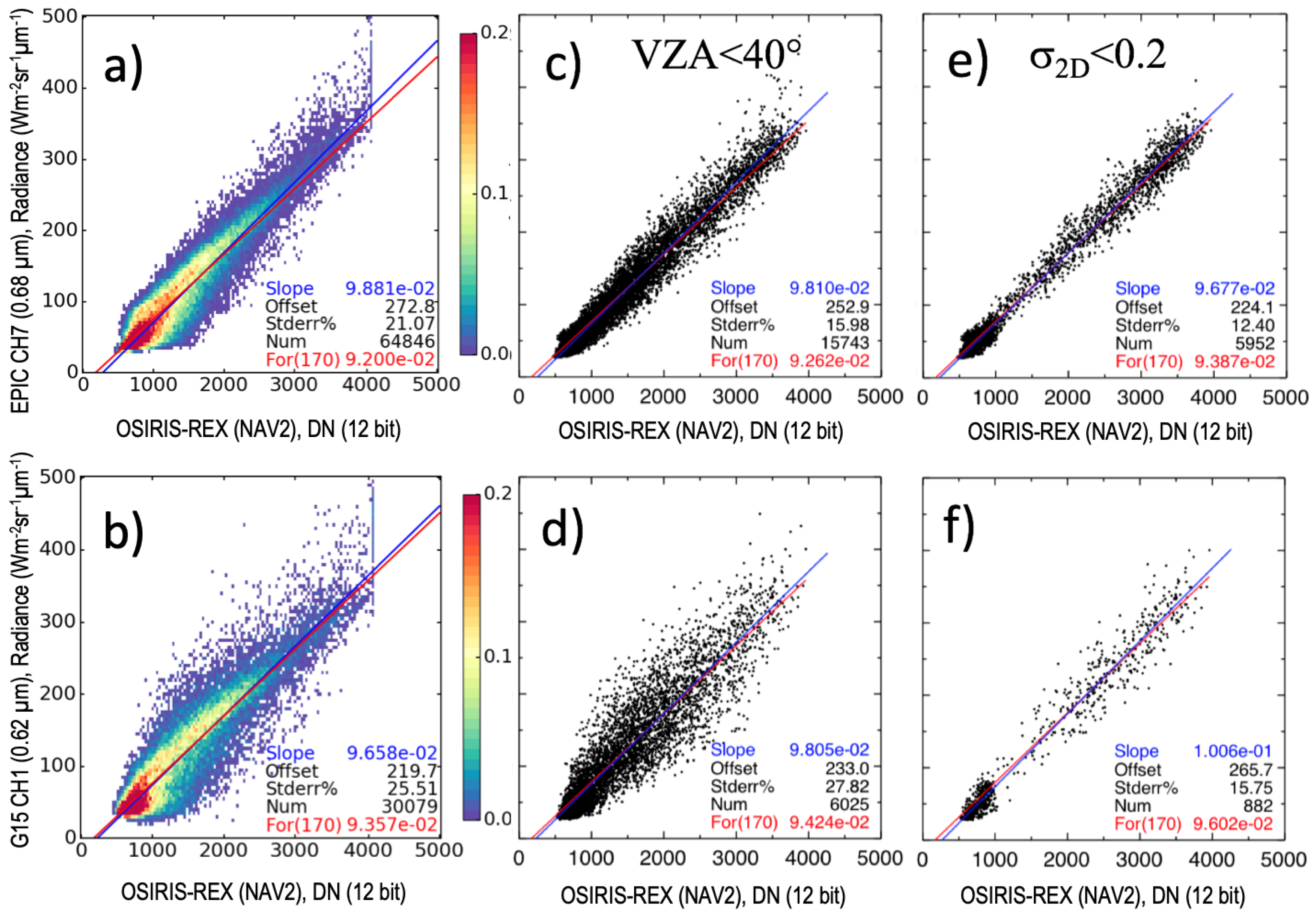
To assess the impact of angle matching tolerance on the NavCam 1 gains, the three GOES-15 images were matched with a sequence of NavCam 1 images, which were coincident within seven (rows 2–5), two (rows 6–8), and three (rows 9–11) minutes. The GAM angular thresholds were consistent for each sequence of NavCam 1 images. The top half angular thresholds were nearly the same; however, the 1st quartile angular thresholds were the most restrictive for the 22:05 GMT NH image (rows 9–11), less restrictive for the 21:13 GMT FD image (rows 2–5), and the least restrictive for the 21:35 GMT NH image (rows 6–8). The NavCam 1 gain standard deviations for each GOES-15 NH image are 0.2% (22:05 GMT, most restrictive), 0.5% (21:13 GMT, less restrictive), and 1.3% (21:35 GMT, least restrictive). As expected, increasing the angular threshold tolerance increases the uncertainty in the gain. The fact that the NavCam gains are consistent across a sequence of images and that the Earth was centered across various locations in the NavCam field of view suggests that the NavCam 1 CMOS flatfielding is very good.
To determine whether the angular thresholds were effective, the ATO-RM gains are compared to the top half radiance gains (>200), which have a more Lambertian reflection than ATO, for the ten GOES-15/NavCam 1 images (rows 2–11). The ATO-RM minus the ATO-RM top half (>200) gain was –0.4%, thus confirming adequate angle matching across the dynamic range. To evaluate the SBAF gain impact, the ATO-RM minus the ATO-RM no SBAF (noSB) gain was +1.5%. The NavCam 1 10-image average ATO-RM and ATO-RM no SBAF offsets were 164 and 278, respectively. The ATO-RM offset nearly equals the space DN of 170, which suggests that the application of SBAF when performing ATO-RM mitigated the spectral band differences. The NavCam 1 10-image average standard errors for ATO-RM and ATO-RM no SBAF are 12.0% and 12.7%, respectively. The consistency between the ATO and >200 gain, a regression offset that nearly equals the space DN, and the reduction of the standard error all indicate that both the SBAF and angular matching criteria were sufficient.

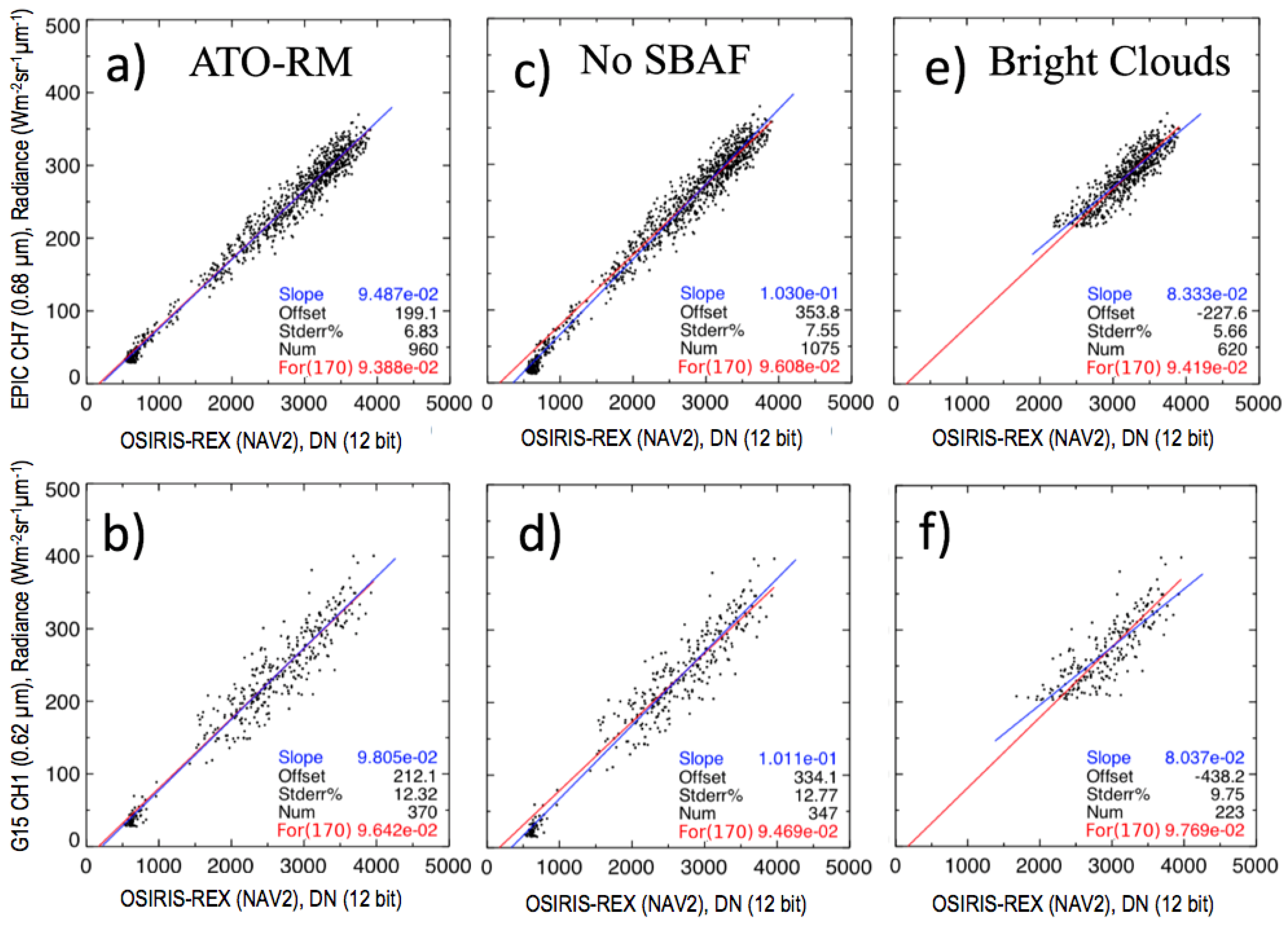
5.2. NavCam 2 Calibration Gains

The last two NavCam 2 images provide an opportunity to assess the impact of the NavCam exposure time settings on the ATO-RM algorithm. Figure 7a,b display the last two NavCam 2 images and can be compared to the first NavCam 2 image shown in Figure 1b. The 3 NavCam 2 images were inter-calibrated with the same GOES-15 NH image. The pixel pair density plots reveal similar features as Figure 5b but are compressed (Figure 7c) or expanded (Figure 7d) across the NavCam DN axis. A total of 75% of the Figure 7b NavCam 2 image pixels are saturated.
The NavCam 2 pixel DN and GOES-15 radiance ATO-RM pairs are displayed in Figure 6b and Figure 7e,f. Figure 6b and Figure 7e have the GAM and σ2D thresholds applied, whereas Figure 7f simply splits the radiance range at 75 Wm−2sr−1µm−1 and applies a σ2D < 0.3. Figure 7e is very consistent with Figure 6b where the standard error and offset are nearly identical. The exposure time ratio for these two NavCam 2 images is 2 = 0.1528 × 10⁻³/0.0764 × 10−3 s. The Figure 7e and Figure 6b NavCam 2 force fit gain ratio is 1.9996, which is nearly identical to the exposure time ratio. The NavCam 2 saturated image lacks the bright cloud pairs and must exclusively rely on the 1st and 2nd quartile radiances, which require stricter angular matching but only broad angular matching is geometrically possible with this NavCam 2 and GOES-15 image configuration. The 1st quartile radiances are not sufficiently matched in angle and therefore do not intersect the force fit line, and the regression standard error was not significantly reduced with the ATO-RM thresholds. The force fit gain is a much better estimate than the slope gain, since it only solves for the gain rather than the gain and offset simultaneously, which may introduce bias in the gain [38]. For this case, the NavCam exposure time ratio is 0.473 = 0.3228 × 10⁻³/0.1528 × 10−3 and the ATO-RM force fit gain ratio is 0.491, which is within 3.9%. The NavCam ATO-RM force fit gains are able to provide consistent gains within 3.9% across exposure times of a factor of ± 2.

6. NavCam 1 ATO-RM Gain Discussion

It is difficult to estimate the true NavCam 1 gain given a very limited number of inter-satellite matches. The twelve NavCam 1 images were matched with two EPIC and three GOES-15 images. Each of the GOES-15 images was matched with multiple NavCam 1 images. The average NavCam 1 gain based on the ten GOES-15 and two EPIC matches is 9.831 × 10⁻² Wm−2sr−1µm−1DN−1 ± 2.2%. Some of the NavCam 1 gain differences may be due to the intrinsic GOES-15 and EPIC radiance value difference. If the EPIC gain were first radiometrically scaled with the GOES-15 gain based on the NavCam 2 22:38:27 image using a scaling factor of 9.642 × 10⁻² (GOES-15)/9.388 × 10−2 (EPIC) = 1.0271, then the NavCam 1 mean gain is 9.874 × 10⁻² Wm−2sr−1µm−1DN−1 ±1.8%. The GOES-15/MODIS ATO-RM radiances are considered more accurate than the EPIC/MODIS ATO-RM radiances, due to the large EPIC navigation error, narrow EPIC band 7 SRF, and greater matching time difference.
The ATO-RM calibration gain uncertainty is based on many factors. For this study, the NavCam barrel lens distortion, flat-fielding, and linear response were not considered. The ground-to-orbit Aqua-MODIS calibration reference uncertainty for band 1 is 1.65% [39]. The MODIS calibration drift adds another 1% [40]. The Figure 1b GOES-15 calibration uncertainty is 1.1% (Section 2.2). The SBAF standard error is 1.9% (Section 4.1). The NavCam 1 12-image gain standard deviation is 1.8% (after scaling the EPIC radiance to GOES-15) and is considered the ATO-RM algorithm uncertainty. The spatial matching error is estimated by the linear regression slope uncertainty. The slope uncertainty is considered the upper limit of the matching error, given the spatial matching error increases the radiance pair noise along with angular mismatching. The slope uncertainty of Figure 6a,b was 0.50% and 1.41%, respectively. The spatial mismatch error is estimated at 1.41%. The resulting ATO-RM calibration gain uncertainty is 3.71% for the NavCam 1 calibration gain of 9.874 × 10⁻² Wm−2sr−1µm−1DN−1.

7. Comparison with Pre-Launch Calibration

Prior to launch, the radiance responsivities of the two NavCams were characterized at Malin Space Science Systems (MSSS) using an integrating sphere illuminated with a quartz-tungsten-halogen (QTH)–based broadband light source [4]. Due to the broad SRF of the NavCam imager, the pre-launch calibration was derived in terms of in-band radiance by integrating the sensor response over the pass band of the NavCam SRF. In addition, the pre-launch calibration coefficients are normalized by the mean exposure time to facilitate the radiometric comparison of NavCam images acquired at different exposure times. The pre-launch radiometric gains for NavCam 1 and NavCam 2 were estimated to be 100,965 (DN/s)/(Wm−2sr−1) and 102,685 (DN/s)/(Wm−2sr−1), respectively.
The in-flight calibration results based on the ATO method are compared with the pre-launch values to identify any temporal drift in the radiometric responsivity of NavCams after launch. The ATO-based radiometric gains of NavCam 1 and NavCam 2 are derived in the units of spectral radiance and are found to be 9.874 × 10⁻² Wm−2sr−1µm−1DN−1 (Section 6) and 9.642 × 10⁻² Wm−2sr−1µm−1DN−1 (Table row 14), respectively. These gains are multiplied by the equivalent width (343 nm) of the NavCam SRF to adjust to the units of in-band radiance [41]. By further normalizing these gain values by the imaging exposure time (0.1528 × 10⁻³ s), the ATO gains for NavCam 1 and NavCam 2 turn out to be 193,237 (DN/s)/(Wm−2sr−1) and 197,886 (DN/s)/(Wm−2sr−1), respectively. These numbers are significantly higher than the ground-based calibration.
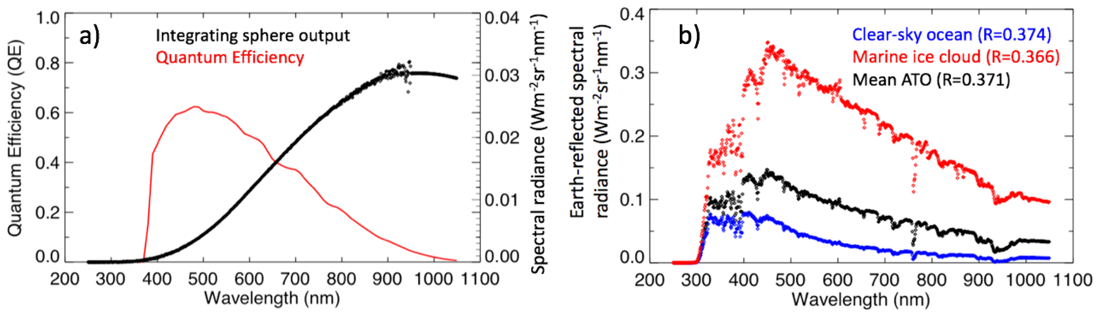
The integrated in-band response of an imaging sensor is dependent upon the illuminating spectra. Figure 8a shows the reference spectral radiance coming out of the exit port of the integrating sphere that was used for the pre-launch calibration. The reference spectra maximize at near-infrared wavelengths where the quantum efficiency (QE), plotted in red, of the NavCam imaging sensor is very small. On the other hand, the ATO-RM method utilizes the Earth-reflected solar spectra that have a peak in the visible part of the spectrum, where the QE also maximizes. To facilitate a direct comparison between the ground-based and in-flight calibration results, the difference in the two reference spectra must be taken into account. A correction factor is derived using the relative ratio (R) of the in-band sensor response to the total over pass band input radiance for each reference spectrum, as defined by the following equations:
RSphere = [LSphere(λ) × QE(λ) dλ]/[LSphere(λ) dλ]
RATO = [LATO(λ) × QE(λ) dλ]/[LATO(λ) dλ]
where LSphere and LATO are the spectral radiance spectra at the integrating sphere output and the Earth-reflected ATO spectra, respectively, and QE is the quantum efficiency of the sensor. The integration is performed over the spectral range of the filter pass band. The value of RSphere is computed to be 0.198. The Earth-reflected ATO spectra are a combination of the clear-sky ocean and bright cloud targets. Figure 8b shows the top-of-atmosphere spectral radiance spectra of clear-sky ocean, marine ice cloud, and ATO scene conditions derived from SCIAMACHY footprints. It is interesting that the value of R is nearly the same (within 2%) for the clear-sky, marine ice cloud, and the combined ATO spectra. This is because the relative spectral distribution of the reflected solar energy is nearly the same for these scene types. So, the mean ATO spectrum is used for correction. The value of RATO is found to be 0.371. The NavCam 1 ATO gain after correcting for the difference in input spectra is, therefore, computed as:
GainATO(NavCam 1) = 193,237 (DN/s)/(Wm−2sr−1) × (RSphere/RATO) = 103,129 (DN/s)/(Wm−2sr−1)
The adjusted NavCam 1 and pre-launch gain differ by only 2.1%. Similarly, the NavCam 2 ATO calibration of 197,886 (DN/s)/(Wm−2sr−1) is adjusted and found to be 105,610 (DN/s)/(Wm−2sr−1), which is consistent with the pre-launch gain within 2.8%. As a final check on the ground calibration, the ratio of the pre-launch NavCam 1 and NavCam 2 gains (0.9833) was compared with the ATO-RM gain ratio (0.9765) and was found to be within 0.7%. The consistent pre-launch and on-orbit NavCam gains denote a stable performing sensor, while in space.

8. Conclusions

The Earth-viewed OSIRIS-REx NavCam images captured during an EGA maneuver provided an opportunity to validate the NavCam pre-launch ground-based calibration. GOES-15 and DSCOVR-EPIC imager radiances were found most suitable to inter-calibrate the NavCam images. First the GOES-15 and EPIC pixel-level radiances were mapped to the EPIC field of view. An optimized ATO-RM inter-calibration algorithm accounted for spectral band differences, navigation errors, radiance field changes due to the time matching difference, and angular geometry differences by incorporating SBAFs, spatial homogeneity tests, and radiance stratified angle matching thresholds.
Twelve NavCam 1 images were inter-calibrated with two EPIC and three GOES-15 images, which were first radiometrically scaled to the Aqua-MODIS reference calibration. The GOES-15 reference radiances were considered more accurate than the EPIC reference radiances, owing to the large EPIC navigation error, exceptionally narrow SRF, and greater matching time difference. After radiometrically scaling the EPIC radiances to GOES-15, the NavCam 1 mean gain is 9.874 × 10⁻² Wm−2sr−1µm−1DN−1 ± 1.8%. After accounting for known uncertainties in the NavCam ATO-RM algorithm, the total gain uncertainty is estimated at 3.7%. The ATO-RM orthogonal regression offset of 164 is close to the true space DN of 170. When strict angular matching thresholds are possible between multiple NavCam 1 and two matched GOES-15 images, the standard deviation of the ATO-RM NavCam gains were within 0.2%–0.5%, suggesting that the NavCam 1 CMOS detector flatfielding is very good. The ATO-RM calibration was able to provide gains that are consistent within 3.9% across a factor of ±2 exposure times. The ATO-RM calibration method can be verified by using both GOES-15 and EPIC to independently transfer the Aqua-MODIS reference calibration to NavCam 2 and the resulting gains were consistent within 2.6%.
The ATO-RM NavCam 1 and NavCam 2 gains were compared with the pre-launch gains. The pre-launch gains were based on using an integrating sphere and a QTH lamp. After accounting for the difference of the solar and lamp spectra, the pre-launch and ATO-RM NavCam 1 and NavCam 2 gains were within 2.1%–2.8%. The estimated ATO-RM gain uncertainty was 3.7%, indicates that the pre-launch and the ATO-RM gain difference is less than what can be significantly resolved using the ATO-RM calibration method. Finally, the NavCam 1 and NavCam 2 calibration gain ratios based on ATO-RM and pre-launch were within 0.7% of each other, indicating consistent NavCam 1 and 2 optical performance while in space. The ATO-RM calibration results verify that the on-orbit NavCam calibration gain is very similar to the pre-launch gain, indicating that no significant NavCam performance changes have occurred during space flight.
This work provides an independent, in-flight absolute radiometric calibration of NavCam 1 and 2. This aided the NavCam exposure time planning for Bennu observations. The small 3% radiometric uncertainty we found also benefits asteroid analyses that rely on absolute radiometric information in NavCam imagery. For example, NavCam images of Bennu provide an independent measurement of the body’s albedo, in concert with the other imagers onboard the OSIRIS-REx spacecraft. It also informs how accurately we can estimate from NavCam images the sizes of unresolved particles ejected from Bennu’s surface. Size measurements of these objects has become important to the OSIRIS-REx mission since their first detection in January 2019 [5].
This study has demonstrated that images of the sunlit Earth disk taken during an EGA maneuver by a solar-system probe, such as OSIRIS-REx, can be inter-calibrated using Earth-orbiting imagers. Due to the limited number of NavCam images and coarse pixel resolution, geostationary imagers are the most suited sensors for this task. The GEO imagers operationally scan at least every half hour and the most current sensors scan a full disk every 15 min. The current constellation of GEO satellites provides contiguous imagery across Earth, which offers inter-calibration opportunities no matter where the probe observes, except over the poles, where GEO satellite views are not possible.

Author Contributions

D.D. formulated and directed the methodology, validation, results analysis, and prepared the manuscript. K.K. referenced the NavCam 1 images with respect to Earth coordinates, mapped and aligned the EPIC and GOES-15 images into the NavCam 1 field of view. C.H. processed, plotted, and analyzed all of the NavCam, GOES-15, and EPIC images. R.B. scaled the NavCam pre-launch and satellite inter-calibration gains. B.B. processed the NavCam images and provided and interpreted the pre-launch NavCam results. B.S. and A.G. determined the SBAF. All authors reviewed the manuscript.

Funding

This material is based upon work supported by NASA under Contract NNM10AA11C issued through the New Frontiers Program.

Acknowledgments

TAGCAMS images are available via the Planetary Data System (PDS) (https://sbn.psi.edu/pds/resource/orex/) [17]. This study was supported by NASA ROSES proposal NNH14ZDA001N-DSCOVR.

Conflicts of Interest

The authors declare no conflict of interest.

References

  1. “OSIRIS-REx Factsheet” (PDF). NASA/Explorers and Heliophysics Projects Division. Available online: https://ehpd.gsfc.nasa.gov/documents/552572main_OSIRIS_REx_Factsheet.pdf (accessed on 26 August 2019).
  2. “OSIRIS-REx The Mission”. Available online: https://www.asteroidmission.org/mission/ (accessed on 26 August 2019).
  3. Lauretta, D.S.; Balram-Knutson, S.S.; Beshore, E.; Boynton, W.V.; Drouet D’Aubigny, C.; DellaGiustina, D.N.; Enos, H.L.; Golish, D.R.; Hergenrother, C.W.; Howell, E.S.; et al. OSIRIS-REx: Sample return from asteroid (101955) Bennu. Space Sci. Rev. 2017, 212. [Google Scholar] [CrossRef]
  4. Bos, B.J.; Ravine, M.A.; Caplinger, M.; Schaffner, J.A.; Ladewig, J.V.; Olds, R.D.; Norman, C.D.; Huish, D.; Hughes, M.; Anderson, S.K.; et al. Touch and Go Camera System (TAGCAMS) for the OSIRIS-REx Asteroid Sample Return Mission Space. Sci. Rev. 2018. [Google Scholar] [CrossRef]
  5. Lauretta, D.S.; Hergenrother, C.W. Episodes of particle ejection from the surface of the active asteroid (101955) Bennu. Science. in press. [CrossRef]
  6. Heidinger, A.K.; Cao, C.; Sullivan, J. Using Moderate Resolution Imaging Spectrometer (MODIS) to calibrate Advanced Very High Resolution Radiometer (AVHRR) reflectance channels. J. Geophys. Res. 2002, 107. [Google Scholar] [CrossRef]
  7. Cao, C.; Weinreb, M.; Xu, H. Predicting Simultaneous Nadir Overpasses among Polar-Orbiting Meteorological Satellites for the Intersatellite Calibration of Radiometers. J. Atmos. Ocean. Technol. 2004, 21, 537–542. [Google Scholar] [CrossRef]
  8. Bhatt, R.; Doelling, D.R.; Scarino, B.R.; Gopalan, A.; Haney, C.O.; Minnis, P.; Bedka, K.M. A consistent AVHRR visible calibration record based on multiple methods applicable for the NOAA degrading orbits, Part I: Methodology. J. Atmos. Ocean. Technol. 2016, 33, 2499–2515. [Google Scholar] [CrossRef]
  9. Doelling, D.R.; Bhatt, R.; Scarino, B.R.; Gopalan, A.; Haney, C.O.; Minnis, P.; Bedka, K.M. A consistent AVHRR visible calibration record based on multiple methods applicable for the NOAA degrading orbits, Part II: Validation. J. Atmos. Ocean. Technol. 2016, 33, 2517–2534. [Google Scholar] [CrossRef]
  10. Heidinger, A.K.; Straka, W.C., III; Molling, C.C.; Sullivan, J.T. Deriving an inter-sensor consistent calibration for the AVHRR solar reflectance data record. Int. J. Remote Sens. 2010, 31, 6493–6517. [Google Scholar] [CrossRef]
  11. Li, C.; Xue, Y.; Liu, Q.; Guang, J.; He, X.; Zhang, J.; Wang, T.; Liu, X. Post calibration of channels 1 and 2 of long-term AVHRR data record based on SeaWiFS data and pseudo invariant targets. Remote Sens. Environ. 2014, 150, 104–119. [Google Scholar] [CrossRef]
  12. Wu, A.; Xiong, X.; Angal, A. Deriving a MODIS-based calibration for the AVHRR reflective solar channels of the NOAA KLM operational satellites. IEEE Trans. Geosci. Remote Sens. 2013, 51, 1405–1413. [Google Scholar] [CrossRef]
  13. Doelling, D.; Haney, C.; Bhatt, R.; Scarino, B.; Gopalan, A. Geostationary Visible Imager Calibration for the CERES SYN1deg Edition 4 Product. Remote Sens. 2018, 10, 288. [Google Scholar] [CrossRef]
  14. Inamdar, A.K.; Knapp, K.R. Intercomparison of Independent Calibration Techniques Applied to the Visible Channel of the ISCCP B1 Data. J. Atmos. Ocean. Technol. 2015, 32, 1225–1240. [Google Scholar] [CrossRef]
  15. Meirink, J.F.; Roebeling, R.A.; Stammes, P. Inter-calibration of polar imager solar channels using SEVIRI. Atmos. Meas. Tech. 2013, 6, 2495–2508. [Google Scholar] [CrossRef]
  16. Marshak, A.J.; Herman, S.; Adam, B.; Karin, S.; Carn, A.; Cede, I.; Geogdzhayev, D.; Huang, L.; Huang, Y.; Knyazikhin, M. Earth Observations from DSCOVR EPIC Instrument. Bull. Am. Meteorol. Soc. 2018, 99, 1829–1850. [Google Scholar] [CrossRef]
  17. Bos, B.; Jackman, C.; Lauretta, D.S. Origins, Spectral Interpretation, Resource Identification, Security, Regolith Explorer (OSIRIS-REx): Touch-and-Go Camera Suite (TAGCAMS) Bundle, urn:nasa:pds:orex.tagcams, NASA Planetary Data System. 2019. Available online: https://pds.nasa.gov/datasearch/subscription-service/SS-20190630.shtml (accessed on 12 November 2019).
  18. Lazzara, M.A.; Benson, J.M.; Fox, R.J.; Laitsch, D.J.; Rueden, J.P.; Santek, D.A.; Wade, D.M.; Whittaker, T.M.; Young, J.T. The Man computer Interactive Data Access System: 25 years of interactive processing. Bull. Am. Meteorol. Soc. 1999, 80, 271–284. [Google Scholar] [CrossRef]
  19. Weinreb, M.; Jamieson, M.; Fulton, N.; Chen, Y.; Johnson, J.-X.; Bremer, J.; Smith, C.; Baucom, J. Operational calibrationof Geostationary Operational Environmental Satellite-8 and -9 imagers and sounders. Appl. Opt. 1997, 36, 6895–6904. [Google Scholar] [CrossRef]
  20. CERES Edition 4 Calibration Coefficients. Available online: https://satcorps.larc.nasa.gov/cgi-bin/site/showdoc?mnemonic=CALIB-ED4 (accessed on 26 August 2019).
  21. CERES Updated Realtime GEO Calibration. Available online: https://satcorps.larc.nasa.gov/cgi-bin/site/showdoc?mnemonic=CALIB-UPRT# (accessed on 26 August 2019).
  22. DSCOVR Earth Sensors Science Team: DSCOVR EPIC Level 1B Dataset. Available online: https://eosweb.larc.nasa.gov/project/dscovr/dscovr_epic_l1b_2 (accessed on 21 November 2018).
  23. Geogdzhayev, I.V.; Marshak, A. Calibration of the DSCOVR EPIC visible and NIR channels using MODIS Terra and Aqua data and EPIC lunar observations. Atmos. Meas. Tech. 2018, 11, 359. [Google Scholar] [CrossRef]
  24. Doelling, D.; Haney, C.; Bhatt, R.; Scarino, B.; Gopalan, A. The Inter-Calibration of the DSCOVR EPIC Imager with Aqua-MODIS and NPP-VIIRS. Remote Sens. 2019, 11, 1609. [Google Scholar] [CrossRef]
  25. 2014: NOAA KLM User’s Guide, Appendix I. Available online: https://www1.ncdc.noaa.gov/pub/data/satellite/publications/podguides/N-15 thru N-19/pdf/ (accessed on 26 August 2019).
  26. Khlopenkov, K.V.; Trishchenko, A.P. Implementation and Evaluation of Concurrent Gradient Search Method for Reprojection of MODIS Level 1B Imagery. IEEE Trans. Geosci. Remote Sens. 2008, 46, 2016–2027. [Google Scholar] [CrossRef]
  27. Khlopenkov, K.V.; Trishchenko, A.P. Achieving Subpixel Georeferencing Accuracy in the Canadian AVHRR Processing System. IEEE Trans. Geosci. Remote Sens. 2010, 48, 2150–2161. [Google Scholar] [CrossRef]
  28. Khlopenkov, K.; Doelling, D.; Okuyama, A. MTSAT-1R visible imager point spread function correction, Part II: Theory. IEEE Trans. Geosci. Remote Sens. 2015. [Google Scholar] [CrossRef]
  29. Chander, G.N.; Mishra, N.; Helder, D.L.; Doelling, D.R.; Aaron, D.B.; Angal, A.; Choi, T.; Xiong, X. Applications of spectral band adjustment factors (SBAF) for cross-calibration. IEEE Trans. Geosci. Remote Sens. 2013, 51, 1267–1281. [Google Scholar] [CrossRef]
  30. Spectral Response Function Database. Available online: https://satcorps.larc.nasa.gov/cgi-bin/site/showdoc?docid=194&c=home2 (accessed on 26 August 2019).
  31. Bovensmann, H.; Burrows, J.P.; Buchwitz, M.; Frerick, J.; Noël, S.; Rozanov, V.V.; Chance, K.V.; Goede, A.P.H. SCIAMACHY: Mission objectives and measurement modes. J. Atmos. Sci. 1999, 56, 127–150. [Google Scholar] [CrossRef]
  32. Scarino, B.D.; Doelling, R.; Gopalan, A.; Chee, T.; Bhatt, R.; Haney, C. Enhancements to the open access spectral band adjustment factor online calculation tool for visible channels. Proc. SPIE 2018. [Google Scholar] [CrossRef]
  33. Scarino, B.R.; Doelling, D.R.; Minnis, P.; Gopalan, A.; Chee, T.; Bhatt, R.; Lukashin, C.; Haney, C.O. A Web-Based Tool for Calculating Spectral Band Difference Adjustment Factors Derived From SCIAMACHY Hyperspectral Data. IEEE Trans. Geosci. Remote Sens. 2016. [Google Scholar] [CrossRef]
  34. GOES-8 through GOES-15 Imager Spectral Response Functions. Available online: https://www.ospo.noaa.gov/Operations/GOES/goes-imager-srfs.html (accessed on 6 November 2019).
  35. Herman, J.; Huang, L.; McPeters, R.; Ziemke, J.; Cede, A.; Blank, K. Synoptic ozone, cloud reflectivity, and erythemal irradiance from sunrise to sunset for the whole earth as viewed by the DSCOVR spacecraft from the earth–sun Lagrange 1 orbit. Atmos. Meas. Technol. 2018, 11, 177–194. [Google Scholar] [CrossRef]
  36. Wielicki, B.A.; Doelling, D.R.; Young, D.F.; Loeb, N.G.; Garber, D.P.; MacDonnell, D.G. Climate quality broadband and narrowband solar reflected radiance calibration between sensors in orbit. In Proceedings of the IGARSS 2008 IEEE International Geoscience and Remote Sensing Symposium, Boston, MA, USA, 7–11 July 2008. [Google Scholar]
  37. Doelling, D.R.; Haney, C.O.; Scarino, B.R.; Gopalan, A.; Bhatt, R. Improvements to the geostationary visible imager ray-matching calibration algorithm for CERES Edition 4. J. Atmos. Ocean. Technol. 2016, 33, 2679–2698. [Google Scholar] [CrossRef]
  38. Ignatov, A.; Cao, C.; Sullivan, J.; Levin, R.; Wu, X.; Galvin, R. The usefulness of in-flight measurements of space count to improve calibration of the AVHRR solar reflectance bands. J. Atmos. Ocean. Technol. 2005, 22, 180–200. [Google Scholar] [CrossRef]
  39. Xiong, X. MODIS Reflective Solar Calibration and Uncertainty Assessment. Available online: http://gsics.atmos.umd.edu/pub/Development/20110322/Day2pm_GRWG_Xiong_MODIS.pdf (accessed on 26 August 2019).
  40. Doelling, D.R.; Wu, A.; Xiong, X.; Scarino, B.R.; Bhatt, R.; Haney, C.O.; Morstad, D.; Gopalan, A. The radiometric stability and scaling of collection 6 Terra- and Aqua-MODIS VIS, NIR, and SWIR spectral bands. IEEE Trans. Geosci. Remote Sens. 2015, 53, 4520–4535. [Google Scholar] [CrossRef]
  41. Solar Constants Comparison. Available online: https://satcorps.larc.nasa.gov/cgi-bin/site/showdoc?mnemonic=SOLAR-CONSTANT-COMPARISONS (accessed on 26 August 2019).
Figure 1. (a) The OSIRIS-REx NavCam 2 22 September 2017 22:38:27 GMT image. (b) The same as (a) except with Earth centered and zoomed at 425 × 425 pixels. The NavCam-relative Earth North and South Poles are located along the upper left and lower right corner diagonal. (c) The 22:30 GMT GOES-15 NH imager visible channel. (d) The 22:41:14 GMT DSCOVR-EPIC band 7 (0.68 µm) image.
Remotesensing 11 02717 g001
Figure 2. The NavCam [17], GOES-15 imager band 1 [34] and EPIC band 7 [35] normalized spectral response functions.
Remotesensing 11 02717 g002
Figure 3. The NavCam 2 22:38:27 GMT (a) viewing zenith angle (VZA) and (b) relative azimuth angle (RAA) images corresponding to Figure 1b. The 22:41:14 GMT EPIC (c) VZA and (d) RAA images corresponding to Figure 1c. The 22:30 GMT GOES-15 (e) VZA and (f) RAA NH images corresponding to Figure 1d). The color bar units are in degrees.
Remotesensing 11 02717 g003
Figure 4. (a) The 22:38:27 GMT NavCam 2 minus 22:41:14 GMT EPIC VZA difference in degrees. (b) The 22:38:27 GMT NavCam 2 minus 22:30 GMT GOES-15 VZA difference in degrees. (c,d) Same as (a) and (b) except with RAA difference in degrees. (e) NavCam 2 image pixel DN where both NavCam 2 and EPIC field of views are limited to a VZA< 40°. (f) Same as (e) except for NavCam 2 and GOES-15. (g) NavCam 2 image pixel DN where both NavCam 2 and EPIC fields of view are ray-matched according to Table 1 row 13 under the GAM top half. (h) NavCam 2 image pixel DN where both NavCam 2 and GOES-15 fields of view are ray-matched according to Table 1 row 14 under the GAM top half.
Remotesensing 11 02717 g004
Figure 5. (a) The 22:38:27 GMT NavCam 2 pixel DN and 22:41:14 GMT EPIC pixel radiance collocated pairs displayed as a relative density plot. The color bar units are in relative frequency. (b) The 22:38:27 GMT NavCam 2 pixel DN and 22:30 GMT GOES-15 pixel radiance collocated pairs displayed as a relative density plot. (c,d) Same as (a) and (b) except for also applying VZA < 40.0 and σ2D < 0.7 thresholds. (e,f) Same as (c) and (d) except including the σ2D < 0.2 threshold. The slope, offset, and stderr% are the orthogonal linear regression gain, x-offset in DN, and associated standard error in percent, respectively. For(170) is the force fit gain or the linear regression through the NavCam 2 space DN of 170. Num is the number pairs for the month.
Remotesensing 11 02717 g005
Figure 6. (a) The 22:38:27 GMT NavCam 2 pixel DN and 22:41:14 GMT EPIC pixel radiance ATO-RM using GAM. (b) The 22:38:27 GMT NavCam 2 pixel DN and 22:30 GMT GOES-15 pixel radiance ATO-RM using GAM. (c,d) Same as (a) and (b) except for without applying SBAF. (e,f) Same as (a) and (b) except excluding radiances < 200 Wm−2sr−1µm−1.
Remotesensing 11 02717 g006
Figure 7. The (a) 22:43:33 GMT and (b) 22:43:41 GMT NavCam 2 images. The sensor exposure time of (a) is half that of Figure 1b and the exposure time of (b) is approximately twice that of Figure 1b. The NavCam 2 DN at 4095 are considered saturated. The (c) 22:43:33 GMT and (d) 22:43:41 GMT NavCam 2 DN and 22:30 GMT GOES-15 pixel radiance collocated pairs displayed as a relative density plot. The color bar units are in relative frequency. (e,f) Same as (c) and (d) except for the ATO-RM pairs. See Figure 5 for explanation of the upper left statistics.
Remotesensing 11 02717 g007
Figure 8. (a) The spectral radiance output (black) from the integrating sphere and the QE plot (red). (b) Comparison of the clear-sky ocean, marine ice cloud, and ATO spectra.
Remotesensing 11 02717 g008
Table 1. lists the individual NavCam image calibration gains. From left to right: The times in GMT in which the NavCam images calibrated in this study were taken on 22 September 2017. The NavCam 2 times are bold. The matched EPIC (E) or GOES-15 (FD, NH) image time is given in GMT. For GOES-15, the time is expressed at the equator. The GAM (VZA, RAA, SCAT) thresholds in degrees are given for the top half and 1st quartile radiances. Shown next are the NavCam gains (Wm−2sr−1µm−1DN−1) based on the ATO-RM (ATO), ATO-RM for radiances <200 Wm−2sr−1µm−1 (<200), and ATO-RM without SBAF applied (noSB). The ATO-RM and ATO-RM without SBAF (no SBAF) orthogonal regression standard errors (σ) are shown in percent and x-offsets (Off) in DN.
NavCamEPIC/GAMGain × 10−2ATO-RMno SBAF
1/2GOES-15top half1st QATO>200noSBσOffσOff
21:08:3020:53:11 E15,20,2010,15,159.4879.5799.66910.922112.5338
21:10:5421:13 FD15,30,2010,25,1510.08010.1109.92013.118714.1312
21:13:1710.04010.0809.87113.519414.7317
21:15:3510.07010.1109.90114.319615.4321
21:20:5210.15010.1909.96113.419814.8322
21:32:0621:35 NH15,30,2015,30,209.9559.9779.81211.611512.0239
21:35:269.7949.8359.65110.813711.4261
21:37:419.7099.7819.55910.418510.9314
22:04:3222:05 NH15,25,205,15,109.6739.7209.54310.815311.2276
22:06:509.7119.7509.57511.513312.0252
22:09:149.7159.7499.57910.114210.6266
22:16:3522:41:14 E15,20,2010,15,159.5849.6099.7846.81357.6279
22:38:2722:41:14 E20,25,3015,20,259.3889.4199.6086.81997.6354
22:38:2722:35 NH25,30,1515,20,59.6429.7699.46912.321212.8334
22:43:3319.28019.54018.99012.121112.7271
22:43:414.7375.3934.33331.254236.7771

