A Review of Progress and Applications of Pulsed Doppler Wind LiDARs
by
 , , and
Zhengliang Liu
1,* ,
,
Janet F. Barlow
2,
Pak-Wai Chan
3, 
Jimmy Chi Hung Fung
4,
Yuguo Li
5,
Chao Ren
6,
Hugo Wai Leung Mak
7 and
Edward Ng
1,† 1
Institute of Environment, Energy and Sustainability, Chinese University of Hong Kong, Hong Kong, China
2
Department of Meteorology, University of Reading, P.O. Box 243, Reading RG6 6BB, UK
3
Hong Kong Observatory, Hong Kong, China
4
Department of Mathematics, Hong Kong University of Science and Technology, Hong Kong, China
5
Department of Mechanical Engineering, University of Hong Kong, Hong Kong, China
6
Faculty of Architecture, University of Hong Kong, Hong Kong, China
7
Faculty of Engineering, Chinese University of Hong Kong, Hong Kong, China
*
Author to whom correspondence should be addressed.
†
Current address: School of Architecture, Chinese University of Hong Kong, China.
Remote Sens. 2019, 11(21), 2522; https://doi.org/10.3390/rs11212522
Submission received: 6 September 2019
/
Revised: 19 October 2019
/
Accepted: 20 October 2019
/
Published: 28 October 2019
(This article belongs to the Special Issue Remote Sensing: 10th Anniversary)
Abstract
:Doppler wind LiDAR (Light Detection And Ranging) makes use of the principle of optical Doppler shift between the reference and backscattered radiations to measure radial velocities at distances up to several kilometers above the ground. Such instruments promise some advantages, including its large scan volume, movability and provision of 3-dimensional wind measurements, as well as its relatively higher temporal and spatial resolution comparing with other measurement devices. In recent decades, Doppler LiDARs developed by scientific institutes and commercial companies have been well adopted in several real-life applications. Doppler LiDARs are installed in about a dozen airports to study aircraft-induced vortices and detect wind shears. In the wind energy industry, the Doppler LiDAR technique provides a promising alternative to in-situ techniques in wind energy assessment, turbine wake analysis and turbine control. Doppler LiDARs have also been applied in meteorological studies, such as observing boundary layers and tracking tropical cyclones. These applications demonstrate the capability of Doppler LiDARs for measuring backscatter coefficients and wind profiles. In addition, Doppler LiDAR measurements show considerable potential for validating and improving numerical models. It is expected that future development of the Doppler LiDAR technique and data processing algorithms will provide accurate measurements with high spatial and temporal resolutions under different environmental conditions.
1. Introduction
Wind field measurements are fundamental observations in several scientific areas such as meteorology and aerodynamics. Numerical simulations, reduced-scale wind tunnel tests and full-scale field measurements are widely adopted in analyzing wind field patterns. Both simulations and wind tunnel tests are only capable of representing part of the reality, and validation and verification are required to assure their respective accuracy and reliability. In contrast, although field measurements have their own limitations, they are able to capture flow features affected by various factors, such as land use, radiation and cloud activities. In addition, field measurements can be taken as references to validate numerical models and wind tunnel tests.
There are several categories of instruments for field measurement of wind flow pattern, and some of them were invented in the 18th and 19th centuries [1]. They are roughly classified into two categories: local anemometers that include mechanical and sonic anemometers, and remote sensors that include Sound Detection and Ranging Devices (SODARs) and Doppler wind LiDARs. While wind measurements carried out by local anemometers have high spatial resolutions and are often considered as references to evaluate the performance of remote sensors, they are limited to a small spatial coverage and limited heights. On the other hand, remote sensors measure air in a probe volume within a large range of spatial coverage. The advantages and disadvantages of several techniques for the purpose of wind measurement are briefly summarized in Table 1.
Doppler LiDAR is a relatively new technique for obtaining wind measurements and was developed rapidly over the past decades [11]. Instead of acoustic energy utilized in SODARs, LiDARs obtain wind field measurements based on the light energy backscattered by aerosols. The primary advantage of Doppler LiDARs is their unique capability to remotely measure atmospheric winds with relatively higher resolutions compared to SODARs [10]. Beneficial from the development of optical fibre amplifiers, the maximum measurement range of modern LiDARs can exceed 10 km. LiDAR measurements can cover a larger spatial region depending on environmental conditions and provide information at different vertical levels.
According to methods used to determine the frequency shift, the Doppler LiDAR system can be divided into two broad categories: coherent (or heterodyne) detection LiDAR and direct detection LiDAR. In the coherent LiDAR systems, frequency shifts are measured by comparing the return signal to a reference signal; while in the direct detection systems, the return signal is filtered or resolved into its spectral components to obtain frequency shifts. Compared to the direct detection system, the coherent detection system has several advantages: (1) Only the spectral components close to the reference signal are unfiltered, therefore the coherent system has high tolerance of background light [12,13]; (2) The uncertainties are independent of temperature and properties of optical components in the system [14]; (3) The enhanced receiver sensitivity reduces the time required for wind measurements [15,16]. In the coherent LiDAR system, the laser beam can be in the form of continuous wave (CW) or pulses [17,18,19]. Pulsed LiDARs have great capacity for remote measurements, e.g., for distances of more than 10 km [20]. Depending on pulse duration and range gate width, pulsed LiDARs have blind measurement regions of tens to several hundred meters near the beam source. Although CW LiDARs do not have such blind measurement regions, their range resolution is poor beyond a few hundred meters [21]. The range uncertainty of CW LiDARs highly depends on the measurement distance. For example, the range uncertainty of a CW LiDAR with a telescope diameter of 500 mm is around 2 m at a distance of 100 m, which increases to more than 200 m at a distance of 1000 m [14].
This paper overviews fundamentals and applications of pulsed coherent Doppler LiDARs. The sections are organized as follows: basic concepts are introduced to offer a glimpse of LiDAR measurements in Section 2; Section 3 gives a report of LiDAR applications in the areas of aerospace, wind energy and meteorology; and in Section 4, challenges and trends for future LiDAR research are discussed.
2. Fundamentals of Coherent Doppler Wind LiDAR
The acronym LiDAR (Light Detection And Ranging) for measurements using light pulses was first introduced in 1953 and developed rapidly due to the invention of high-energy lasers in recent decades [22]. Depending on the interaction processes of the emitted radiation, different types of LiDARs are capable of performing a diverse range of tasks, which include determination of forest density, river bed elevation, as well as measuring atmospheric variables such as particle depolarization (depolarization LiDAR), concentration of various gaseous compounds (absorption LiDAR), organic compounds (fluorescence LiDAR) and winds (Doppler LiDAR) [23,24].
Doppler LiDAR systems that measure wind along the line of sight by determining frequency shifts were first demonstrated in the mid-late 1960s [10]. By 1970s, pulsed coherent LiDARs with a wavelength of 10.6 m has become a choice for wind measurement [25]. For eye safety reasons, solid-state lasers with a wavelength of 2 m are more frequently used in modern LiDAR systems after 1990 [26]. More recently, fibre lasers with wavelengths of 1.5–1.6 m have been used to improve the compactness and efficiency of coherent LiDAR systems [10]. Nowadays, Doppler LiDAR is a powerful technique for measuring wind vectors from ground-based, shipborne and airborne platforms.
2.1. Measurement Principles and Uncertainties
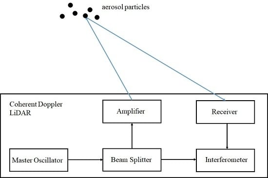
A Doppler wind LiDAR estimates the component of wind velocity projected onto the laser beam propagation direction, named line-of-sight velocity or the radial velocity , based on the measurement of Doppler wavelength shift distribution. The schematic diagram of a coherent Doppler wind LiDAR is shown in Figure 1. In the LiDAR system, the master oscillator laser emits a laser pulse with wave length and frequency , where c is the speed of light. Generally, of a LiDAR system is in the near infrared spectral range (from 1.4 to 2.5 m) to achieve the highest possible transmission of light signals, at the same time ensuring eye safety [27]. The output of the master oscillator laser is split into two parts. The first part seeds an amplifier to create a transmit light beam, while the second part is used as the reference light beam, named local oscillator beam, which may be created by a separate laser in some systems [10]. The radiation transmitted to the atmosphere is backscattered by moving particles, and part of the radiation is captured by the receiving optics. The return signal with frequency is mixed with the reference light in the interferometer. Then the combined single field is focused onto a detector. Using the Doppler shift obtained from the mixed signal by fast Fourier transform or other methods [28,29], the radial velocity is then calculated by
Since the width of the laser beam is finite, the radial velocity is measured in a probe volume along the beam direction. In contrast to CW LiDARs, of which the spatial resolution is dependent on the measurement range, the spatial resolution of pulsed LiDARs is determined by the pulse width and the distance the pulse travels during the sampling time [30]. Although reducing pulse duration can improve spatial resolution, a reasonable sampling duration is required to promise the accuracy of velocity estimation. Currently, the spatial resolution of commercial LiDARs are typically from 30 to 100 m [29]. As shown in Figure 2, if the LiDAR is placed at the origin of the Cartesian coordinate system, the beam orientation is defined in terms of the azimuth angle and the elevation angle . Generally, a set of radial velocity measurements are combined with appropriate assumptions to extract useful information for wind field analysis, such as wind speeds and directions.
The accuracy of estimates is dependent on uncertainties that are tied to the hardware or introduced by atmospheric effects. Due to the nature of coherent detection, prevailing noise in the coherent LiDAR system is proportional to the power of the local oscillator, e.g., relative intensity noise, while noise sources that are independent of the power of local oscillator are negligible [12,19]. Inherent uncertainties of the LiDAR system are also influenced by errors in identifying sensing distance and elevation angle [31]. Environmental conditions, such as turbulence intensity and precipitation, introduce additional uncertainties in velocity measurements. In flat terrain, the turbulence only introduces a random error on the measurement (represented by standard deviation), while in complex terrain, both absolute and relative biases can be introduced. Presence of rain will introduce a strong negative bias on vertical velocities since the radiation backscattered by raindrops will also be measured by the LiDAR system [32].
The ratio between the average signal power and the average noise power, or signal-to-noise ratio (SNR), is commonly used to assess the accuracy of LiDAR measurements [33]. SNR is dependent on both the instrument and atmospheric variabilities within the resolution volume [34]. For example, Gryning et al. [35] found that high SNR was generally associated with high wind speed conditions during long-term measurements. Following Rye and Hardesty [36], Pearson et al. [37] estimated the standard deviation of the Doppler velocity in the weak signal regime using:
where is the ratio of the LIDAR detector photon count to the speckle count; is the spectral width of the signal; is the accumulated photon count; M is the number of points per range gate; and n represents the number of pulses averaged. is explicitly calculated by:
with B being the bandwidth of the receiver. Pearson et al. [37] confined their approximation below −5 dB, and O’Connor et al. [38] found that the influence of SNR on the estimated was insignificant when SNR was larger than 0 dB. The recommended value of was 1.5 m/s and and 2 m/s in the study of Pearson et al. [37] and O’Connor et al. [38], respectively. Since increases monotonically for low values of SNR [38], a tolerable error on can be determined according to such SNR. A threshold SNR, below which data will be discarded, can be provided by the manufacturer or test measurements. Manufacturer Halo Photonics suggests a threshold SNR of −18.2 dB for their StreamLine LiDAR, while tests under quiescent atmospheric conditions suggest a value of −20 dB for the same instrument, resulting in a increase in data availability [34]. In addition, to better estimate the ratio of the wind gust speed to the mean wind speed, Suomi et al. [39] suggested using the spike removal technique instead of SNR threshold for data filtering.
2.2. Scan Patterns
Since a LiDAR system measures the radial velocity, the vertical component of a velocity vector can be directly obtained through a LiDAR measurement at an elevation angle of . To retrieve two-dimensional (2D) or three-dimensional (3D) flow fields, a sequence of radial velocities measured by beams of different directions through LiDAR scanning are required. The scan patterns of LiDAR systems can be categorized according to the number of degree of freedom (DOF) [40].
In the staring mode (zero DOF), the laser beam is fixed in a certain direction. Information obtained from staring is sufficient to estimate SNR [34], vertical wind component [41], backscatter intensity [42] and wind fluctuations in the mean wind direction [43]. In addition, staring can be used in the pre-test to detect regions with high turbulence intensity in turbulence structure studies [44].
Scan patterns in one DOF include complete cone, arc sector and vertical slice scans. In conical scanning, named plan position indicator (PPI) (In some studies, the PPI is also called velocity azimuth display (VAD). In this paper, the VAD is a method for wind retrieval described in Appendix A.1.), is kept constant while the laser beam scans a number of discrete positions within a complete cone (i.e., full ). The PPI scan (see Figure 3a) is the most widely used pattern in LiDAR experiments (see Table A1 in Appendix B). In the arc sector scan in Figure 3b, the laser beam sweeps a range of (less than ) at a constant . Since only a limited range of is scanned, the temporal sampling rate of the arc sector scan is higher than that of PPI [45]. The arc sector scan has been adopted in studies on wind turbine wakes where only flow fields behind the turbine were of interest [46,47]. LiDAR beam can also be swept through a slice, as shown in Figure 3c. This pattern is known as the range height indicator (RHI) and is commonly used in dual or multiple LiDAR systems [48,49,50,51]. In addition, the vertical structure of flow field obtained from RHI scans provides valuable information for the analysis of aircraft/turbine wake features [52,53], as well as for validation of 3D flow features obtained from 2D data [54]. Figure 3d illustrates the scan geometry employed at Hong Kong International Airport to detect the wind shear to be encountered by the airplane [55]. In this scan pattern, the laser beam slides along the glide path.
A typical two DOF scan is Doppler beam swinging (DBS). As shown in Figure 4, several measurements are taken at different along with one measurement in the vertical direction. Since only a few measurements have to be taken, the DBS is fast and simple in terms of hardware and for the purpose of data analysis, but it lacks sufficient information to evaluate the reliability of the results [14]. The minimum requirement of DBS is having 3 orthogonal line of sight scans, i.e., vertical, tilted to the north and tilted to the east respectively. Sathe et al. [56] proposed a DBS scheme with five tilted and one vertical beams, called the “six beam scheme” in their study, and the corresponding retrieval method for calculating six components of the Reynolds stress tensor. Other types of two DOF scans can be made up of a sequence of simple scans [40], e.g., a combination of the staring, PPI, DBS and RHI.
2.3. Methods for Wind Field Retrieval
As a single LiDAR system only measures a single component (i.e., ) of the wind vector (i.e., ) over an area or within a volume, retrieval approaches are commonly required to obtain horizontal components (i.e., u and v) or all three components (i.e., and w) of from the LiDAR observations.
The velocity azimuth display (VAD) [57] and volume velocity processing (VVP) [58] techniques based on the linear least squares regression are widely used to retrieve wind field from LiDAR measurements. In VAD, basis functions are determined by Fourier expansion; while in VVP, basis functions are depending on parameters of interest (i.e., velocity and its gradient). Because of the inherent orthogonality of Fourier series, the VAD is robust. Due to the linear assumption, velocity estimates are normally inaccurate under flow conditions with high nonlinearities [59]. Thus, the number of radial velocity data points and their distribution should be carefully considered to avoid violation of the linear assumption. It is suggested to use equally spaced measurements with five to seven distributed azimuth angles [47,60].
Some efforts have been made to retain the nonlinear properties of the wind field. The optimal interpolation (OI) uses covariance functions and statistical interpolation technique to retrieve wind field [61]. This method can retain local features of the wind field [62] and is suitable for wind retrieval in both simple and complex terrains [63]. Since the estimated covariance function is assumed to hold on a horizontal plane, OI is only valid for wind retrieval at low elevation angles (generally for ). Instead of minimizing the variance of interpolation error in OI, variational methods solve the minimization problem of the cost function [64]. The velocity components can be modeled by orthonormal functions [65] or obtained by minimizing the difference between observations and physical models [66]. Physically based variational methods demonstrate great potential to analyze the performance of computational fluid dynamics (CFD) methods, but are computationally expensive compared to other methods. A detailed description of these retrieval methods is provided in Appendix A.
2.4. Limitations and Precautions
The performance of Doppler LiDARs is significantly affected by four atmospheric factors, namely aerosol backscatter, humidity, precipitation and atmospheric refractive turbulence [67]. The actual range of Doppler wind LiDARs depends on the strength of radiation signals backscattered by aerosol particles. As aerosols above the atmospheric boundary layer (ABL) are in low concentrations, it is beyond the capability of LiDARs to measure the wind velocity above the ABL, except in the presence of desert dust or volcanic plumes at high altitudes [68]. In very clean sky conditions, e.g., after rain brings aerosols to the ground, the returning signal will be too weak for LiDARs to provide meaningful estimates when aerosol particles are absent [69]. The study conducted by Risan [43] indicated that the strength of backscattered signal was proportional to humidity. Iungo et al. [44] suggested increasing the number of laser ray emissions for each velocity profile, as a result enhancing the accuracy even when aerosol concentration is low. Due to strong attenuation of laser beams, the maximum range of LiDARS is limited in fogs and the laser beam cannot penetrate through thick clouds. The maximum horizontal range of LiDARs will decease during sunny days, which is caused by the negative effects of refractive index turbulence on the efficiency of heterodyne detection [68].
As discussed in Section 2.1, the accuracy of a LiDAR system relies on hardware and atmospheric conditions. Therefore, methods for LiDAR measurements should be validated individually against well-defined reference measurements, especially when conditions change, otherwise unanticipated discrepancies may arise [68]. Scan patterns (Section 2.2) and retrieval methods (Section 2.3) also have impacts on bias and precision of the retrieved wind fields. Bonin et al. [70] compared the performance of three scan patterns on turbulence measurements (i.e., turbulence kinetic energy and velocity variances). In their study, DBS measurements provided the best estimates; PPI measurements had a negative bias decreasing with the height; and the precision of RHI measurements was low but their bias was insignificant. In the study on tropical cyclones [71], wind velocities retrieved by the VVP were problematic in high gradient regions, i.e., the tropical cyclone center. Thus, it is important to select appropriate scan patterns and retrieval methods according to desired flow properties and their applications.
Site or platform conditions should also be taken into consideration during LiDAR measurements. If the view of a site is limited by obstacles such as buildings and trees, a larger should be adopted to decrease the impacts of the obstacles. In addition, signals originating from obstacles need to be excluded from measurements [68]. To reduce influences of electromagnetic radiation (e.g., by mobile radio or cellular phone networks), the LiDAR system should be shielded properly [68]. It is suggested to install the LiDAR system at least 3 m above the ground, preferably on a grass-covered ground, to reduce impacts of turbulence on its performance [68]. When the LiDAR system is installed on a ship, motion stabilization system is necessary to derive reliable measurements [72]. For the airborne LiDAR system, corrections to beam directions are required to compensate for aircraft roll and pitch angles [73].
3. Applications of Doppler Wind LiDARs
Pulsed Doppler LiDARs developed by scientific institutes such as Deutsches Zentrum für Luft- und Raumfahrt (DLR), literally German Center for Aviation and Space Flight, and National Oceanic and Atmospheric Administration (NOAA) and commercial companies such as Leosphere (France), Halo Photonics (UK) and Lockheed Martin Coherent Technologies (USA) have been used worldwide to study wake vortices (e.g., generated by an aircraft, a wind turbine or a building), strong wind phenomena (e.g., wind shear and cyclones), and aerosol backscatters. Representative examples in the areas of aerospace, wind energy and meteorology are provided in this section.
3.1. Aviation Safety
Takeoff and landing are considered the most difficult stages of flight. According to existing database, more than half of aviation accidents occurred at these two stages [74]. Many of these accidents are related to the complex flow conditions near the airport, which have important impacts on aircraft performance during takeoff and landing. Doppler wind LiDARs are installed in around a dozen airports to detect wake vortices and dangerous wind shears [27].
3.1.1. Aircraft Wake Vortex
Strong vortices generated by a heavy aircraft (see Figure 5) are potentially hazardous to other flying vehicles. Real-time detection and tracking positions and intensities of wake vortices are prerequisites to optimize separation distances dynamically, which potentially reduce accidents and increase airport capacity. In addition, it provides valuable information for aircraft design. Up to now, Doppler wind LiDAR is the only device recommended by the International Civil Aviation Organization (ICAO) for vortex detection in clear air [75].
Several techniques have been developed to derive the strength of wake vortices from LiDAR measurements. The velocity envelope method extracts the positive and negative velocity envelopes with the aid of a spectrum threshold [77]. The threshold is dependent on SNR and the circulation, which needs to be fine-tuned to optimize the performance of the envelope method. The vortex core position can be determined from the extrema of the velocity spectrum. The vortex circulation is calculated by integrating the envelope in a specified area near the vortex core, e.g., radius of region between 5 m and 15 m. The radial velocity method proposed by Smalikho and Banakh [78] solves several minimization and maximization problems that identify the distance between the LiDAR and the vortices. The vortex circulation is obtained by fitting the velocity measured by LiDAR to that computed by the Burnham-Hallock vortex model. In the study conducted by Smalikho et al. [79], the radial velocity method and the velocity envelope method showed similar performance in predicting the vortex position, while the error of vortex circulation estimated by the radial velocity method was 5 times higher. Computationally expensive methods that make use of estimators on spectrum-based analytical models are more accurate. For example, the bias in vortex circulation given by the maximum likelihood estimator was found to be less than [80]. Since estimator-based methods take signal response functions into consideration, they are suitable for vortex identification when SNR is low [75]. To provide accurate vortex estimation in a reasonable time frame, a hybrid method was developed to use the velocity envelopes to locate aircraft wake vortices and employ the maximum likelihood algorithm to estimate the vortex circulation [81]. The root mean square error in circulation estimated by such hybrid method was less than [82].
In the past three decades, LiDAR measurements have provided extensive data collection for the analysis of vortex formation, movement and decay. According to long-term measurements obtained by Doppler LiDARs, at least 3% of wake vortices generated by landing aircraft is within a distance of 25 m to the following aircraft at Charles de Gaulle airport [83]. Körner and Holzäpfel [84] analyzed 8052 aircraft landings recorded by Doppler LiDARs at several international airports, concluding that 3.7% of the landing vortices were generated below 50 m. To artificially accelerate wake vortex decay or destruct wake vortices for the purpose of aviation safety, it is crucial to uncover the physical mechanism of wake vortex decay, particularly during landing phase and the touchdown process. LiDAR observations indicated that continuous vortex decay was associated with strong turbulence [85] while the two-phase decay, i.e., an initial phase of moderate decay followed by a phase of rapid decay, occurred in weakly turbulence environments [86], corroborating the vortex evolution found in corresponding CFD simulations [87]. With the help of LiDAR measurements, it was found that the radii of vortex cores were almost constant during the decay process [88] and this process could be accelerated by ground effects [75]. To increase the decay rate of wake vortices, Holzäpfel et al. [89] suggested installing a plate line on the ground surface. A reduction of 3% in the lifetime of strong vortices was recorded by a Doppler LiDAR, demonstrating the capacity of surface modification for vortex decay acceleration [89]. With increasing understanding of wake vortices generated by aircraft, new separation standards based on dynamic detection and individual wake characterisation are expected to be implemented worldwide in the foreseeable future [90].
3.1.2. Low Level Wind Shear
Low level wind shear, defined as the sudden change of wind velocity and/or direction in 600 m by the ICAO, may be associated with the frontal surface, convective clouds, microbursts, surrounding terrain, or thermal instabilities. It may affect aircraft performance and present a hazard to aviation safety [91]. Reliable and timely alerts can help pilots to recognize quickly and respond appropriately when wind shear occurs. Over recent years, the Doppler LiDAR technique has been verified to be effective in low-level wind shear alerting under clear air conditions.
The first Doppler LiDAR System for wind shear alerting was installed at the Hong Kong International Airport in August 2002. Chan and his collaborators [55,92,93,94,95,96] have conducted comprehensive studies on wind shear events observed by the LiDAR system, which is a part of the wind shear and turbulence warning system at the Hong Kong International Airport. An automatic wind shear detection algorithm dependent on glide path scan (Section 2.2) has been developed and successfully applied for detection and alerting of terrain-induced wind shear [55]. Hit rates of around 70%, defined as the ratio of the number of wind shear alerts based on the headwind profiles measured by the LiDAR system to the number of wind shear reported by pilots, were achieved for several departure and approach corridors when the availability of LiDAR data was promised [92]. When the headwind gradient was introduced into the alert system by a windshear hazard factor, the hit rate increased to more than 80% [94,95]. Then, a simple smoothing algorithm was employed to reduce the time cost in processing headwind data, resulting in a similar performance as in the previous study using flight simulator software for data smoothing [96].
In the last decade, LiDAR systems for wind shear detection have been tested at several international airports besides the Hong Kong International Airport. Yoshino [97] analyzed the flight record data and LiDAR measurements from PPI scans, concluding that the low level wind shear recorded at the Narita International Airport on 20 June 2012 was caused by horizontal roll vortices. At the Lanzhou Zhongchuan International Airport, wind shear conditions observed by a Doppler LiDAR in PPI scan mode with an elevation angle of were used to assist an aircraft to modify its flight path on 31 May 2016 [27]. At the Beijing Capital International Airport, DBS scans were used to retrieve background wind field, and the step-wise scans shown in Figure 6 were used to identify wind shear events [91]. During the field campaign in 2015 and 2016, more than 2000 scans were analyzed and 14 wind shear events identified from LiDAR measurements were confirmed by pilot reports [91].
As discussed in Section 2.4, raindrops have negative effects on LiDAR performance. Therefore, Doppler radars, which perform well in the rain, should be incorporated into the alerting system to detect wind shear in rainy days [98]. In addition, in case of less common weather conditions, such as fog, other measurement systems are required. A wind shear alert system based on the LiDAR system, the terminal Doppler weather radar, ground-based anemometers, weather buoys and wind shear warnings issued by the aviation weather forecasters has demonstrated its capability for detecting severe wind shear events at the Hong Kong International Airport, covering more than 90% wind shear events reported by pilots from 2002 to 2015 [99].
3.2. Wind Energy
Due to the rapid development of wind industry, wind farms are being built both further offshore and in complex terrain, leading to increasing research on assessment of wind resources under inhomogeneous flow conditions. To better estimate potential power output in different terrains, Wagner et al. [100] suggested using wind speed measurements at different heights instead of the hub-height wind speed measurement. However, conventional in-situ measurements commonly used in the wind energy industry are only capable of characterizing the wind velocity at a limited number of measurement locations. Remote sensors, such as LiDARs, provide promising alternatives to the in-situ techniques for wind measurements at the turbine hub height and beyond. The ability of Doppler LiDAR to measure wind vector remotely is beneficial to the assessment of wind resources, the understanding of wake physics and turbine control.
3.2.1. Wind Resource Assessment
Analysis of wind resources is desired before installation of wind turbines as well as during their operations. In recent years, LiDAR technique has grown in popularity for wind resource assessment because it can quantify wind velocity at several vertical levels to investigate possible impacts on turbine power output.
Kim et al. [101] evaluated the performance of a pulsed Doppler LiDAR for wind resource assessment in three different kinds of terrains on Jeju Island. In their study, the ruggedness index (The ruggedness index is defined as the percentage fraction of the terrain along the prevailing wind direction over a threshold slope [102]. A threshold slope of 0.3 was assumed in [101].) was introduced to identify the complexity of a given terrain. Results showed that the differences in ten-minute averaged wind speed between LiDAR measurements and mechanical anemometer measurements in terrains with ruggedness indices of 2.91%, 2.05% and 0% were 6.02%, 4.75% and 2.23%, respectively [101]. Based on LiDAR measurements, Krishnamurthy et al. [103] generated an averaged wind map on a terrain layer at the hub height of 80 m within an area of around 100 km, locating a region that showed great potential for power production, where the mean wind speeds were higher than 12 m/s. Then, the spatial distribution of wind speeds was applied in a simple topology gradient algorithm to optimize a wind farm layout that maximizes power output. According to their results, the estimate of power output based on wind speed measurement at the hub height (i.e., 80 m) is 0.49% lower than that based on a combination of wind speeds measured at three different heights, as shown in Figure 7. Therefore, they suggested predicting potential power output based on wind profiles at several vertical levels.
As a part of the European Wind Atlas project [104], a series of experiments including the Kassel, Reducing Uncertainty of Near-shore wind resource Estimates (RUNE), Østerild, Terry LiDAR and Perdigão experiments have been conducted in different terrains in Europe. These experiments aimed at evaluating the performance of numerical models for estimating site-specific wind resources in Europe. The Kassel experiment [105] conducted in 2014 demonstrated the capability of multi-LiDAR configuration for measuring turbulent flow in forested complex terrain, providing valuable data to validate forest models. In 2015 and 2016, the RUNE experiment [106] was conducted at the west coast of Denmark close to a test station of wind turbines. Besides providing database for model validation, this campaign aimed at evaluating the performance of different strategies on near-shore wind measurements. Results showed that ten-minute averaged wind speeds estimated by LiDARs in PPI and arc-sector scan modes compared well with those measured by dual-LiDAR systems. In addition, the data availability of ground-based LiDARs in the PPI scan mode was the highest, generally above 95%. In the experiment performed at Østerild test station for large wind turbines in 2016 [107], Doppler LiDARs were installed on the balconies of light towers at 50 m and 200 m above the ground. Data obtained from horizontal scans at 50 m above the ground were categorized according to the inflow velocity measured from a sonic anemometer situated at 37 m above the ground. Analysis of the wind categories along with tree and terrain height maps indicated that mean wind speeds over flat and bare terrains, i.e., non-vegetated areas and water bodies, were higher than those over forested terrains. In the Ferry LiDAR experiment [108], a shipborne LiDAR system was deployed to measure the wind speeds and directions along a regular ferry route across the Baltic Sea from 7 February to 8 June 2017. The initial analysis revealed that low-level jet events occurred more frequently in spring than in winter, owing to the huge difference in temperature between the land and the sea. In the Perdigão 2017 campaign [109], 49 meteorological towers, 27 LiDARs and many other sensors were deployed in the valley and on the two parallel ridges to capture multiscale flow interactions. Initial results indicated that the interaction of synoptic flow with the complex terrain led to surprisingly complex microscale flows.
Due to the complexity of engineering structures in marine environments, deployment of a meteorological tower for assessment of nearshore or offshore wind resources is extremely expensive. As an attractive and applicable alternative to meteorological towers, Doppler LiDARs have been mounted on different platforms to measure wind speeds and directions over the sea. Shimada et al. [110] used two ground-based LiDARs to investigate coastal wind modifications, known as the fetch effect, to determine the optimal distance from the coast for a nearshore wind farm. Their results indicated that the wind speed increased with the increase of the fetch length within 5 km of the coast. They suggested installing wind turbines a few kilometers away from the coast. To assess offshore wind resources efficiently, preliminary measurements can be taken by shipborne [111] or airborne [112] LiDARs within a large region. Then, ground-based [113] or floating [114] LiDARs may be used for obtaining long-term measurements at selected sites.
3.2.2. Turbine Wake
Since turbine induced wakes can reduce power output and increase structural fatigue of downstream turbines, a better understanding of wake properties is helpful in optimizing the performance of wind turbines and the layout of wind farms. Moreover, by taking into account the influence of turbine wakes in wind resource assessment process, predictions of future power production will likely be improved [115]. Doppler LiDAR is an ideal instrument to measure turbine wakes that cover a large downstream volume [116], which has been applied to investigate wakes generated by an individual turbine as well as interactions between multiple turbine wakes [117,118].
In the Turbine Wake and Inflow Characterization Study (TWICS) experiment [119,120,121] took place at the National Wind Technology Center in Colorado in 2011, a high-resolution Doppler LiDAR developed by the National Oceanic and Atmospheric Administration (NOAA) was used to investigate wakes generated by a 2.3 MW turbine with a rotor diameter of 101 m and a height of 80 m. According to data from arc sector and PPI scans, Smalikho et al. [119] found that the lengths of wind turbine wakes ranged from 120 m to 1180 m under different atmospheric conditions. They concluded that the wake length was proportional to the turbulence energy dissipation rate. The study of Aitken et al. [120] focused on analyzing the velocity deficit and the wake boundaries. It was shown that the vertical deficit was 50–60% immediately behind the turbine and reduced to 15–25% at 657 m away from the turbine. The vertical width of turbine wakes increased significantly slower than the horizontal width because of the presence of ground. Banta et al. [121] developed procedures to characterize the 3D structure of turbine wakes and presented a case study based on the data sampled in the TWICS experiment. In their study, maximum deficits of up to 80% were observed at 60 m–200 m behind the turbine rotor.
The Crop Wind Energy Experiment (CWEX) [122,123,124] was conducted within a wind farm with 200 1.5-MW turbines in central Iowa in United States. In summer 2011, flux stations and Doppler LiDARs were deployed to investigate the atmospheric influence of wind turbines on surrounding crops. It was found that wind turbine wakes modified the surface micro climate, resulting in higher CO flux down into the crop canopy during daytime and higher temperature during nighttime [122]. Analysis of wind velocities measured upwind and downwind of a turbine indicated that wake propagation was sensitive to inflow wind direction [123]. The maximum velocity deficit was observed near the hub height at different inflow wind speeds, consistent with existing research results [123]. Mirocha et al. [124] validated CFD simulations implemented with the generalized actuator disk (GAD) model against the CWEX observations in the near wake region, and concluded that the GAD model was unable to capture the variance of the streamwise velocity.
Iungo et al. [44] measured wakes generated by a 2-MW turbine located in Canton de Valais, Switzerland, and observed a sharp increase in turbulence at the turbine top tip height. This represents a typical feature of wind turbine wakes and has been observed in wind tunnel tests [125] and numerical simulations [126]. In the LiDAR experiment conducted in the offshore wind farm Alpha Ventus in Germany, Bastine et al. [127] observed homogeneous isotropic turbulence in the inner wake region of a wind turbine under the free flow condition of anisotropic turbulence. The isotropic turbulence might result from the formation of a new turbulent cascade near the rotor, hence the flow features inside the turbine wake are independent of the surrounding atmospheric flow [127]. In the same wind farm, Dorren et al. [128] tested a non-synchronous dual LiDAR system and demonstrated the capacity of their proposed multiple-LiDAR wind field evaluation algorithm for turbine wake measurements. LiDAR experiments conducted in three wind farms in China from 2013 to 2015 indicated that the differences in velocity deficit, wake length and dissipation rate between day and night were significant, while the difference in turbulence intensity was insignificant [129].
In the Smart Rotors to Improve Wind Energy Efficiency and Sustainability (SMARTEOLE) project, two nacelle-mounted LIDARs were deployed to investigate wakes generated by two wind turbines [117]. It was observed that the turbine wakes were aligned with the wind direction, and the far wake of the upstream turbine merged with the wake generated by the downstream turbine. The CWEX campaign in 2013 focused on a region characterized by strong diurnal cycles of atmospheric stability and frequent jets [118]. Doppler LiDARs were deployed to study wakes generated by a row of four turbines, as shown in Figure 8. The results indicated that the velocity deficits of the outer turbines was lower than that of the inner ones. Moreover, outer turbines showed larger angular changes of wake centerlines, which were related to the wind veer, compared to the inner ones [118].
3.2.3. Turbine Control
Wind turbine control is widely used in the wind energy industry to ensure long structural life and efficient performance of wind turbines operating under complex environmental conditions [130]. In recent decades, Doppler LiDAR technique has received considerable interest in the possibility of improving wind turbine control by providing look-ahead wind measurements in front of the rotor plane [131].
Nacelle mounting and spinner mounting are two main options for LiDAR installation [21]. The numerical study conducted by Bossanyi et al. [132] indicated that the performance of nacelle mounted LiDAR and spinner mounted LiDAR was similar. Although the rotating blades can block the laser beam at some instant, nacelle mounted LiDAR is popular for turbine control due to its simplicity since a proof-of-principle experiment in 2003 [21]. The first spinner mounted LiDAR was deployed in the spinner of a 2.5 MW wind turbine in the “Tjæreborg Spinner-lidar Experiment” in 2009 [133]. CW LiDARs were used in the pioneered experimental studies in 2003 [21] and in 2009 [133]. In the past few years, field tests [134,135] also demonstrated the capacity of pulsed LiDARs mounted on turbine nacelle for upstream wind measurements (Figure 9). In addition, numerical simulations indicated pulsed LiDARs were suitable for spinner mounting configuration in turbine control applications [132,136].
Generator torque control, yaw control and blade pitch control are three typical strategies of wind turbine control [137]. In the LiDAR-assisted control system, the PPI scan pattern is generally used and the optimal scan configurations are dependent on control objectives. For example, in the study of Bossanyi et al. [132], LiDAR scanning at smaller , i.e., larger half cone angle between the laser beam and the centerline, provided better wind direction estimates, which were important for yaw control; while the accuracy of estimated longitudinal wind speed and shear gradients was worse. Schlipf et al. [138] used a brute force method to search for the optimal scan configuration for collective pitch feedforward control, noting that the pulsed LiDAR performed well when it scanned at a half cone angle of , with 6 beam directions, the first range gate at 0.625 rotor diameter and a range gate distance of 0.125 rotor diameter.
Simulations conducted by Schlipf et al. [139] showed that the improvement in power output by introducing LiDAR measurements to assist variable speed control was insignificant since the standard variable speed control was already well optimized. In addition, the torque control strategy led to a dramatic increase in loads on the shaft [140]. Experimental and numerical studies indicated that yaw control and pitch control could benefit from wind fields obtained from LiDAR measurements [131]. Fleming et al. [135] estimated an increase of 2.4% in annual energy production if LiDAR data was used to correct wind vane measurements in yaw control. LiDAR-assisted pitch control can improve rotor speed regulation as well as reduce structural loads [141]. Bossanyi et al. [132] performed simulations to investigate collective pitch control and individual pitch control, concluding that both control strategies were improved by LiDAR measurements.
3.3. Meteorological Research
Doppler wind LiDAR is well suited to measure boundary layer and mesoscale variations in the wind field, which are essential to meteorology and climate studies [142]. An individual Doppler LiDAR system can measure atmospheric parameters such as boundary layer height and wind profiles, while more meteorological quantities can also be obtained when Doppler LiDAR is collocated with other devices. Full-scale wind field measurements are helpful in the improvement and validation of numerical models.
3.3.1. Boundary Layer
Observations of the mixed layer height (MLH) are helpful to improve weather and air quality predictions since MLH is an important parameter in numerical modeling of pollutant dispersion [69] and cloud development [41]. Two LiDAR based parameters, i.e., the velocity variance and backscatter coefficient, can be used to derive MLH [37,143]. Since the velocity variance is more closely connected to the driving process of entrainment, it will provide better estimates of MLH [144]. Through comparing with 141 MLHs derived from radiosonde measurements with the bulk Richardson number method, Schween et al. [69] concluded that the velocity variance was more appropriate for MLH estimation than the aerosol backscatter coefficient. Barlow et al. [145] observed that the backscatter-derived boundary layer lagged approximately two hours behind the velocity-derived boundary layer, as shown in Figure 10. However, when the velocity variance was poorly defined due to the weakly unstable conditions over the water, aerosol backscatter was useful to estimate MLH [146].
Due to the blind measurement region near the beam source of pulsed LiDARs, vertical velocity variance derived from data measured by a LiDAR in staring or scan modes with high elevation angles were insufficient to identify boundary layers below the minimum measurement range. In the experiment conducted in 2015 and 2016, Vakkari et al. [147] derived the MLH from radial velocity variance measured by PPI scans at low elevation angles. Their results showed that the MLHs estimated from PPI scans compared well with those estimated from vertical staring when there was overlapping coverage. In the experiment, MLH was below the lowest vertical range for more than 40% of the time at Limassol, Cyprus and Loviisa, Finland [147]. To take advantage of different scan patterns, Bonin et al. [148] proposed a fuzzy logic–based composite technique to estimate MLH from the surface up to several kilometers. They applied this technique to analyze the MLH in suburban Indianapolis in 2016, revealing that the afternoon MLH was larger around the summer solstice, while the nocturnal MLH was larger in winter because of stronger near-surface winds in winter. In contrast, Halios and Barlow [149] found that the night-time MLH in London was lower in winter than that in summer, reflecting the annual cycle of thermal forcing.
Hogan et al. [150] used higher order moments such as vertical velocity skewness to reveal “upside down” convective mixing caused by stratocumulus clouds. Harvey et al. [151] went on to develop a boundary layer classification scheme to better understand the physics of boundary layer dynamics based on the backscatter coefficient, the vertical velocity skewness and the vertical velocity variance estimated from LiDAR measurements, as well as the surface flux measured by a sonic anemometer. Analysis of data measured by a vertical staring LiDAR and a sonic anemometer at the Chilbolton Observatory in southern England from 1 June 2008 to 31 May 2011 indicated that the stable boundary layer with clear skies was the most common type, occurring 40% of the time [151]. Following Harvey et al. [151], Manninen et al. [152] proposed a method to classify turbulent mixing within the boundary layer and identified a turbulent source with the aid of the attenuated backscatter coefficient, the vertical velocity skewness, the dissipation rate of turbulent kinetic energy, the vertical profiles of horizontal wind, and the vectorial wind shear estimated from LiDAR measurements. Analysis of data measured at Hyytiälä, Finland and Jülich, Germany in 2015 and 2016 showed that surface-driven convection was a dominant source of turbulent mixing during spring, summer and autumn. In addition, low level jets were also an important source of nocturnal mixing [152].
3.3.2. Urban Meteorology
Doppler LiDARs are suitable for operation in urban areas, with focus on detecting aerosols emitted from human activities. Besides urban boundary layer identification [42,143,149,153,154], they have also been deployed to measure wind speeds in urban areas.
Drew et al. [155] deployed a Doppler LiDAR to determine wind speed profiles over central London from May 2011 to January 2012, aiming at evaluating models to assist calculations of potential wind loading on buildings. It was found that the mean wind speed during the entire experiment fitted well with a logarithmic wind profile below 1000 m. Above 1000 m, the wind speed increased sharply and deviated significantly from the logarithmic profile. In addition, the wind profile during low wind speed periods where neutral conditions occurred 6% of the time showed poor agreement with the logarithmic profile, while that during high wind speed periods where neutral conditions occurred 30% of the time compared well with the logarithmic profile. By comparing results of Engineering Sciences Data Unit (ESDU) models with LiDAR measurements in strong wind conditions, Drew et al. [155] suggested conducting assessments regarding the nature of urban surface when ESDU models are adopted to estimate urban wind profiles, as a result the wind loading on tall buildings can be effectively calculated. In the study of Kent et al. [156], wind speeds predicted by a logarithmic model, the Deaves and Harris model, a non-equilibrium model, the power law and the Gryning profile were extrapolated to 200 m above the canopy for comparison with LiDAR observations. When the height variability estimated by morphometric models was taken into consideration, results of the Deaves and Harris model and the Gryning profile showed better agreement with LiDAR measurements compared to all other considered models [156]. Sepe et al. [157] used the vertical wind profiles measured by a Doppler LiDAR to search for optimal parameters in the logarithmic model and the Deaves and Harris mode, via curve fitting approaches. Although the optimized logarithmic model and Deaves and Harris model compared well with experimental data, the optimal values of roughness length were tied to the wind direction and were larger than standard values adopted in the field of wind engineering. In addition, both models overestimated the amount of turbulence [157]. LiDAR measurements taken in Aversa, Italy during the period from October 2015 to July 2016 were used to optimize parameters of the logarithmic model and the Deaves and Harris wind model [157]. It was found that when the mean wind speed at 50 m was less than 4 m/s, the wind direction changed frequently due to thermal effects, while the variability of the wind direction was small when the wind speed exceeded 10 m/s [157]. To better estimate approaching wind velocity in wind-driven ventilation assessment, a Doppler LiDAR was placed on a building rooftop in Tokyo to determine the wind profile [158,159]. It was found that the power law index for estimating the potential of natural ventilation was time dependent, having a value of 0.2–0.3 in evenings, nights and mornings, but decreasing to less than 0.1 during daytime because of the diurnal cycle in convection [158]. In addition, the power law produced poor estimates of wind profiles under low wind speed conditions due to significant deviation in wind direction at different altitudes [159].
Wood et al. [160] investigated airflow channeling along the River Thames with a Doppler LiDAR for better understanding of ventilation within central London. The speed of the air flow over the river showed obvious diurnal variation on sunny days, while the variation on cloudy days was insignificant [160]. On 27 May 2008, a well-developed sea-breeze front was observed in the Tokyo metropolitan area [161]. The propagation speed of the sea breeze estimated from Figure 11 was 4.7 m/s, which was higher than that of 3.7 m/s predicted by a theoretical model. A strong updraft with the maximum vertical velocity of 5 m/s was observed when the sea breeze front was approaching the LiDAR, as shown in Figure 11b. Another sea breeze was captured by a Doppler LiDAR in the Fukuoka–Kitakyushu metropolitan area on 11 September 2015 [162]. The observations were used to evaluate the performance of the Weather Research and Forecasting model when it was combined with different land-use datasets [162].
3.3.3. Tracking Atmospheric Flows
Doppler LiDARs are capable of investigating intense wind phenomena such as cyclones, because they possess relatively high spatial and temporal resolutions. Several studies have employed combined systems including Doppler LiDARs and other devices to gather certain information, e.g., mass flux, in the atmosphere.
During the Observing system Research and Predictability Experiment (THORPEX) Pacific Asian Regional Campaign (T-PARC) in 2008, airborne LiDAR systems were first applied to observe Typhoon Nuri [163] and Typhoon Sinlaku [164]. Afterwards, airborne LiDAR systems were employed to collect wind profiles in Hurricane Earl (2010) [165], Tropical Storm Erika (2015) [166], and Tropical Cyclones Danny (2015), Erika (2015), Earl (2016), and Javier (2016) [71]. In these studies, LiDAR measurements showed good agreement with dropsonde measurements. In the study of Zhang et al. [166], a tilt of the Erika vortex was observed when the altitude was greater than 750 m, as shown in Figure 12. Compared to a typical hurricane, the boundary layer in the Tropical Storm Erika was deeper and the asymmetry of the tangential and radial winds in Erika was more significant.
In 2009 and 2010, a Doppler LiDAR and a X-band Doppler radar was mounted on a truck to identify tornadoes in Oklahoma, Texas, Kansas and Colorado respectively. It was found that the tornadogenesis was not correlated with the appearance of horizontal convective rolls or their orientations. In southwestern Germany, 12 extratropical cyclones were observed by a ground-based LiDAR in 2016 and 2017 [167]. Initial results indicated that wind gusts might be caused by sting jets or convection embedded in the cold front [167].
As a part of the German Vertical Transport and Orography project, an airborne Doppler wind lidar, a rawinsonde, a dropsonde, a wind-temperature radar, a ground-based aerosol LiDAR, and two pilot balloons were used to analyze the vertical structure of Alpine pumping. The mass flux quantified by the Doppler LiDAR indicated that the entire layer of air up to 1900 m between Munich (80 km north of the Alps) and the Alpine rim was transported to the Alps on a sunny day in summer (19 July 2002) [168]. Kiemle et al. [73] measured latent heat fluxes over the Black Forest mountains with water vapour differential absorption and Doppler wind LiDARs installed on a Falcon research aircraft. Their results showed that the latent heat flux was roughly constant with height, while varied significantly between flight legs in the range of 100–500 W/m [73]. A Doppler wind LiDAR and in-situ instruments, including particle impactors were used to investigate the properties of the ash plume from the Eyjafjalla volcano [169]. During the period from April to May 2010, the volcano emitted about 3 Tg of SO and spread over large parts of Central Europe. The ash mass concentrations derived from measurements were used to predict ash loading and support aviation agencies, especially for their airspace decisions when volcanic ash is present, for example air traffic decisions and judgments [169].
3.3.4. Model Validation and Improvement
Validation is a crucial part in terms of numerical studies. It is important to validate numerical models before their corresponding predictions can be adopted in complicated assumptions and initial conditions. Davies et al. [42] compared boundary layer heights determined by national and local air-quality forecasting models with corresponding LiDAR observations of 5 days. They found that both models overestimated the boundary layer height by 100% in the day prior to thunderstorms [42]. Risan et al. [43] validated detachment eddy and Reynolds-averaged Navier–Stokes simulations against LiDAR measurements in complex terrain. In their study, velocities were measured directly in the direction aligned with the mean flow velocity (staring pattern in Section 2.2) to avoid errors introduced by retrieval methods. Chen [170] investigated the air flow that passed through a tall cylinder building in Tainan with the aid of LiDAR measurements and CFD simulations, and emphasized the importance of inflow boundary conditions in CFD simulations.
Some efforts have been made to use LiDAR measurements to improve the accuracy of numerical models [171]. Pu et al. [163] evaluated the performance of an advanced research version of the Weather Research and Forecasting model [172] in predicting the formation and intensity of Typhoon Nuri. They found that when the model was initialized with the wind field retrieved from airborne Doppler LiDAR measurements, better numerical predictions were obtained. A comprehensive study [164] on assimilation of LiDAR measurements in global models for typhoon forecasts showed that LiDAR observations led to a 9% reduction of 12 h–120 h track errors in the European Centre for Medium-Range Weather Forecasts (ECMWF) modeling system. Moreover, an improvement of 3% in 2–4 day forecasts of geopotential height over Europe was achieved when LiDAR measurements were assimilated in the ECMWF modeling system [173].
4. Summary and Outlook
Remote sensors are appealing alternatives to traditional anemometers for wind field measurements. Doppler LiDARs estimate the radial velocity by measuring the frequency shift between a reference laser beam (i.e., local oscillator beam) and the radiation backscattered by aerosols. Due to their capabilities to estimate atmospheric parameters from a large distance, Doppler LiDARs have been installed on ground-based, airborne, shipborne and truck-mounted platforms and undertake different tasks. Corresponding studies show great potential of Doppler LiDARs for aeronautical, wind energy and meteorological applications.
Since a Doppler LiDAR only measures radial velocities, some assumptions are required to retrieve three velocity components of the wind field from LiDAR data (Section 2.3). In single LiDAR applications, the uncertainties of LiDAR measurements over complex terrain are of great importance, where the homogeneous assumption used in retrieval methods is violated. Many efforts have been made to correct LiDAR data based on linear models or CFD simulations. An improvement of around 1.5% can be achieved when the LiDAR measurements are corrected with a flow model for the inhomogeneities [174]. However, the performance of model corrections is case dependent, which may result from insufficiently specified terrain complexity. Therefore, it is suggested to validate LiDAR measurements individually against well-defined reference measurements, especially in complex terrains. In addition, numerical simulations can be conducted in advance of a measurement campaign to support the experiment design under local conditions. Another way to reduce uncertainties related to inhomogeneous flow is the use of multi-LiDAR configuration. The major drawback of synchronized multi-LiDAR measurements is the low availability of data due to blockage (e.g., the available data from dual LiDARs scanning ridges was 50–70% [175]). Recently, new LiDAR systems with three spatially separated emitters [176] or with three receiving units [177] have been developed to measure 3D wind vector with high spatial and temporal resolutions. These systems show considerable potentials for conducting wind measurements in complex terrain, as well as for gust detection where high temporal resolution is desired. To pave the way for LiDAR applications in the airborne wind shear detection and alert system, or the nacelle-based wind turbine control system, Doppler LiDAR technique needs to be better developed to meet cost, size and weight constrains.
Doppler LiDARs have played important roles in uncovering the physical mechanism of formation and decay of aircraft induced vortices, and they have shown remarkable performance for vortex detection. In particular, the probability of detecting an aircraft induced vortex in the first LiDAR scan was found to be about 94% in a 9-month experiment at Lanzhou Zhongchuan Airport [27]. Further investigations on vortex behavior are expected to support the concepts of dynamic distance separation of aircraft and acceleration of wake vortex decay. Data from Doppler LiDAR can provide insights to long-distance vortex transport, the interaction of wake vortices with the ground and influences of atmospheric conditions on vortex intensity. These studies will pave the way for quantification of the degree of vortex hazard and prediction of the vortex lifetime, thus serving as prerequisites for dynamic separation. Although several field campaigns have demonstrated the capacity of Doppler LiDARs for wind shear detection and alert, it is difficult to evaluate the performance of Doppler LiDARs quantitatively, because the intensity and location of wind shear reported by pilots is highly dependent on their experience. Further analysis of long term wind shear statistics based on data recorded by airborne sensors, ground-based ultrasonic anemometer and Doppler LiDARs is necessary to improve the hit rate of wind shear alert. In addition, airborne LiDARs at cruise altitude show great potential for improving air data system reliability and flight safety, such as providing a sufficient advance warning of air dynamics hazards. Moreover, studies that focus on fulfilling functional needs from pilot points of view will be beneficial to the ongoing development of commercial airborne LiDAR systems.
In the wind industry, Doppler LiDARs have been accepted as alternatives of the traditional mast-based wind sensors for wind resource assessment, power performance estimation and turbine wake analysis. Doppler LiDARs are popular for offshore applications because of their mobility and capacity to measure wind remotely. According to the report on International Energy Agency (IEA) Wind Task 32, the use of Doppler LiDARs to detect and measure complex flow, to estimate second-order statistics for load verification and to assist turbine control has to be further developed [178]. As mentioned previously, incorporating numerical models in reconstruction of wind fields from LiDAR measurements will generally provide better estimates. However, the development of combining simulation outputs and LiDAR measurements, as well as methods for uncertainty estimation is still at an early stage. Clear guidance on scan pattern choice, model correction and uncertainty characterization are required to support LiDAR practices and standards in the wind industry. Since most models were originally developed over land, more offshore observations are suggested to validate and improve these models for offshore applications. Long-term records of wind variations, e.g., caused by storms, gusts or coastal irregularities, will be helpful to estimate the wind loading in fatigue testing of turbine blades. Due to the multidisciplinary nature of turbine control, scan patterns and retrieval methods have to be optimized to satisfy data requirements for the control system, e.g., quick assessment of the rotor effective wind speed. Taking full advantage of the pulsed Doppler LiDAR scanning over a large spatial area, LiDAR-based algorithms targeted at controlling the entire wind farm would be helpful to maximize power output and reduce damages caused by severe wind events.
Doppler LiDARs provide possibilities to better understand atmospheric wind, to improve numerical forecasts, and to validate models with more available observations. It is a challenging task to deduce atmospheric turbulence from raw LiDAR data, especially from near ground measurements, where the influence of probe volume averaging is significant. Development of scan patterns and corresponding retrieval methods for turbulence measurement is still an active research topic in the last two decades [179]. In the future, synchronized multi-LiDAR configurations and LiDAR systems with three emitting or receiving units may provide possibilities to remove the impediment to turbulence measurements, thus improving our understanding of turbulence. Due to the high concentration of aerosol, Doppler LiDAR is a promising technique for boundary layer and wind measurements in urban areas, especially above the urban canopy. LiDAR measurements are expected to provide valuable information in studies on urban ventilation, air pollution dispersion, sea breezes, heat island and flow disturbances caused by tall buildings. Wind profiles obtained by Doppler LiDARs would considerably improve the setting up of initial and boundary conditions for conducting numerical simulations, particularly in complex circumstances, such as assessing ventilation at the pedestrian level. In addition, measurements of winds, temperature and moisture profiles with a deployment of instruments including Doppler LiDARs are valuable for model validations.
Author Contributions
Conceptualization: Z.L., J.F.B., P.-W.C., J.C.H.F., Y.L., H.W.L.M., C.R., E.N.; Methodology: Z.L., J.F.B., H.W.L.M, P.-W.C.; Formal Analysis: Z.L., J.F.B., H.W.L.M.; Writing-Original draft preparation: Z.L.; Writing-Review and Editing: H.W.L.M., J.F.B.; Supervision: J.F.B., E.N.; Funding acquisition: E.N.
Funding
This research received no external funding.
Acknowledgments
We thank the reviewers for the constructive comments which helped us a lot in the revision of paper and in making a better presentation of our work.
Conflicts of Interest
The authors declare no conflict of interest.
Abbreviations
The following abbreviations are used in this manuscript:
| 2D | two-dimensional |
| 3D | three-dimensional |
| 4DVAR | four-dimensional variational data assimilation |
| CFD | computational fluid dynamics |
| CW | continuous wave |
| CWEX | Crop Wind Energy Experiment |
| DBS | doppler beam swinging |
| DLR | Deutsches Zentrum für Luft- und Raumfahrt |
| DOF | degree of freedom |
| ECMWF | Medium-Range Weather Forecasts |
| ESDU | Engineering Sciences Data Unit |
| ICAO | International Civil Aviation Organization |
| LiDAR | Light Detection And Ranging |
| MLH | mixed layer height |
| NOAA | National Oceanic and Atmospheric Administration |
| OI | optimal interpolation |
| PPI | plan position indicator |
| RHI | range height indicator |
| RUNW | Reducing Uncertainty of Near-shore wind resource Estimates |
| SNR | Signal-to-Noise Ratio |
| SODAR | Sound Detection and Ranging Device |
| TWICS | Turbine Wake and Inflow Characterization Study |
| VAD | velocity azimuth display |
| VVP | volume velocity processing |
Appendix A. Wind Retrieval Methods
This section describes retrieval methods based on the linear least squares regression (velocity azimuth display in Appendix A.1 and volume velocity processing in Appendix A.2) and two data assimilation techniques (optimal interpolation in Appendix A.3 and variational methods in Appendix A.4). Methods to retrieve wind fields from datasets obtained by multiple LiDARs are discussed in Appendix A.5.
Appendix A.1. Velocity Azimuth Display
Based on the assumption that the wind field is horizontally homogeneous, the basic idea of the velocity azimuth display (VAD) is to fit the observed wind velocity at a given elevation angle to a sinusoidal curve [180]. Assuming that the velocity vector varies linearly around the center of the circle being scanned, the first order Taylor approximation of 3 velocity components are given by
where , and are velocity components at the center of the circle being scanned by LiDAR. As shown in Figure A1, the Cartesian coordinates is converted to the spherical coordinates by
Here r denotes the radial distance from the LiDAR, is the elevation angle and is the azimuthal angle. The radial velocity is expressed as:
Neglecting vertical derivatives, i.e., and , and derivatives of w in Equation (A4) gives a Fourier series in :
with coefficients:
When n radial velocity observations (, ) are obtained, Equation (A4) is converted to:
where is the parameter vector that consists of basis functions; is the combination of Fourier coefficients; and represents the model error. Then, a linear least squares regression can be used to estimate , which is related to the velocity components and kinematic information of the wind field. If the flow is assumed to be uniform, can be calculated using the first harmonics in Equation (A5).
Figure A1.
Schematic overview of Doppler LiDAR used to measure wind profiles. is the wind velocity vector at the measurement point, is the reference velocity vector at the center of the circle being scanned by LiDAR, is the radial velocity, r is the radial distance from the LiDAR, is the elevation angle, and is the azimuthal angle.

Appendix A.2. Volume Velocity Processing
Instead of using Fourier series (Equation (A5)), volume velocity processing (VVP) technique determines a set of basis functions that are dependent on desired parameters. With the assumption that varies linearly with (the same as the VAD in Appendix A.1), the vector that consists of all kinematic parameters K is denoted by:
and the vector of corresponding functions P is given by:
Similar to VAD described in Appendix A.1, the least squares fit is employed to estimate . The primary difference between the VAD and VVP lies on the method to choose parameters (i.e., ) and the corresponding basis functions (i.e., ). In VVP, is not inherent orthogonality, which may lead to numerical instability. To cope with this problem, Boccippio [181] suggested to neglect vertical shear terms (i.e., ). The diagnostic analysis shows that the influence of neglecting vertical shear terms is insignificant and can be further mitigated by increasing spatial resolution in the vertical direction, i.e., z direction [181].
Appendix A.3. Optimal Interpolation
In the optimal interpolation (OI), the wind velocity is projected onto the analyzed coordinate system (). As shown in Figure A2, the l axis is parallel to and the t axis is perpendicular to the l axis. is the angle between the x axis and the l axis. and are components of in the l and t directions, respectively. Velocity components are related to through , where denotes the rotation matrix [182]. The covariance function of velocities, i.e., and at positions and respectively, is defined as
where is the statistical mean. If strict isotropy holds true [61], the relation between covariance tensors in the and the coordinate systems is given by:
where and are diagonal elements of the covariance tensor . With the assumptions of homogeneity and isotropy, elements in are functions of and are independent of . Similarly, the covariance function of the radial velocity is given by
where is the velocity component perpendicular to the radial velocity .
Figure A2.
Decomposition of velocities at two points and .

To determine the covariance function , it is further assumed that the observation errors are uncorrelated with background errors and are not auto-correlated when , where represents the range of observation error correlation [183]. The innovation correlation is defined as [183]:
where is the normalized innovation of the ith observation point; is the innovation; is the observed radial velocity; is the background radial velocity; is the innovation variance; and is the averaged innovation variance over all available observations points. The background field can be provided by another instrument [183] or retrievals from VAD [62,103]. Then, the background error covariance matrix and observation error covariance matrix are estimated based on the innovation correlation in the range of and , respectively [62].
Based on the assumption that the background and observation errors are Gaussian random and independent of each other [184], the variational cost function is written as:
where is the vector of desired variables in the analysis space; is the vector of background information in the analysis space; is the vector of observations in the observation space; and are respectively the background and observation error covariance matrices; and is the matrix consisting of linear observation operators that maps vectors in the observation space to the corresponding analysis space [61]. To minimize the cost function in Equation (A14), the velocity increment should satisfy the following two conditions [185]:
where is a vector containing n normalized innovation defined previously. The increment in can be obtained with:
Appendix A.4. Variational Methods
In variational methods, weak or penalty constraints can be directly added to the cost function. According to models that compute analytical variables in Equation (A14), variational methods can be classified into two types [186]: function fitting-based methods, e.g., two-step variational method (2SVAR); and physical-based method, e.g., four-dimensional variational data assimilation (4DVAR).
In the 2SVAR, the cost function is defined as:
where is predicted by control functions; is the background velocity; is the grid spacing; and denotes summation over a 2D space. The third, fourth and fifth terms on the right hand side of Equation (A17) are smoothing terms involving divergence, vorticity and Laplacian of the velocity field, respectively. The last term is a conservation constraint [93]. The weights in Equation (A17) are chosen to ensure all the terms having the same order of magnitudes [186]. To model velocity components (), the second order orthonormal functions are employed:
where and are Legendre polynomials [187]. The first step of the 2SVAR is to determine coefficients and for , which can be done via minimizing the cost function in Equation (A17) by setting . Then, based on the background velocity field obtained in the previous step, a similar minimization procedure is adopted to retrieve the velocity field.
In the 4DVAR, the cost function is defined as:
where is predicted by the incompressible Navier–Stokes equations; and denotes summation over time and 3D space, respectively; is the temperature; and is a coefficient related to the quality of the observational dataset. The second term on the right hand side of Equation (A19) is a penalty constraint to suppress divergence of the initial field with [188]. is adjusted dynamically to ensure the contribution of the last term is less than . Due to the unpredictable nature of turbulence, the impact of background variables is difficult to predict and is omitted in the 4DVAR system [188]. A gradient-based optimization method is employed to minimize the cost function in Equation (A19) [189].
Appendix A.5. Retrieval Methods of Multiple LiDARs
In order to fully characterize the wind vector , three linearly independent measurements are required. Efforts have been made to combine space and time synchronized measurements from two or three LiDARs at different locations. Figure A3 illustrates a dual LiDAR scan with 4 intersecting points. Multi-LiDAR configurations can improve time resolution by sampling the same volume simultaneously from different directions, thus decrease the uncertainties caused by inhomogeneity of fluid [40].
Based on simple trigonometry, Collier et al. [190] computed velocity components at a limited number of intersecting points of two LiDAR beams. A similar method was used by Calhoun et al. [48] and Cheynet et al. [191] to retrieve the wind field by solving 2D linear equations. This idea provides a simple way to calculate velocity components on the plane determined by the intersecting laser beams. Since only two linearly independent have been measured, the linear system with three orthogonal velocity components (i.e., and w) is underdetermined. In order to obtain 3D wind fields from dual LiDAR observations, Drechsel et al. [50] and Newsom et al. [192] incorporated the incompressible continuity equation (i.e., ) into the linear system by employing a central difference numerical scheme or by minimizing a cost function. When dual LiDAR observations were used in 4DVAR retrievals, the accuracy of 4DVAR increased from 80–90% to 90–94% compared to the single LiDAR system.
A semi-synchronized system with three LiDARs was used by Berg et al. [193] to increase the temporal resolution of mean wind estimates. In the study on instantaneous wind estimates [194], the turbulent quantities measured by three LiDARs staring at a point close to a sonic anemometer compared well with corresponding sonic anemometer measurements. In synchronized trinal LiDAR configurations, 3D wind velocity variance can be directly obtained by solving 3D linear equations [195,196].
Figure A3.
Schematic diagram of a dual LiDAR scan. Blue solid circles represent the intersecting points of two LiDAR beams.
Figure A3.
Schematic diagram of a dual LiDAR scan. Blue solid circles represent the intersecting points of two LiDAR beams.

Appendix B. Summary of Literature on Pulsed Doppler Wind LiDARs

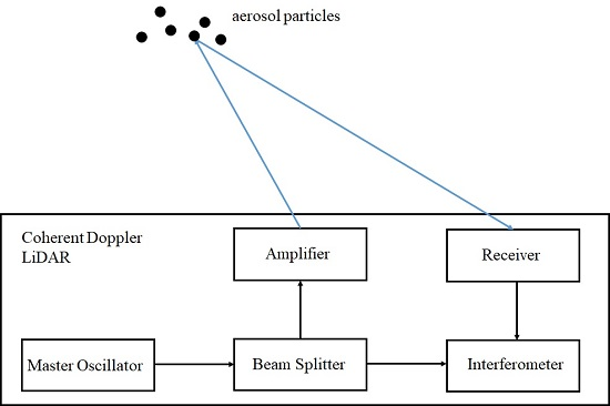
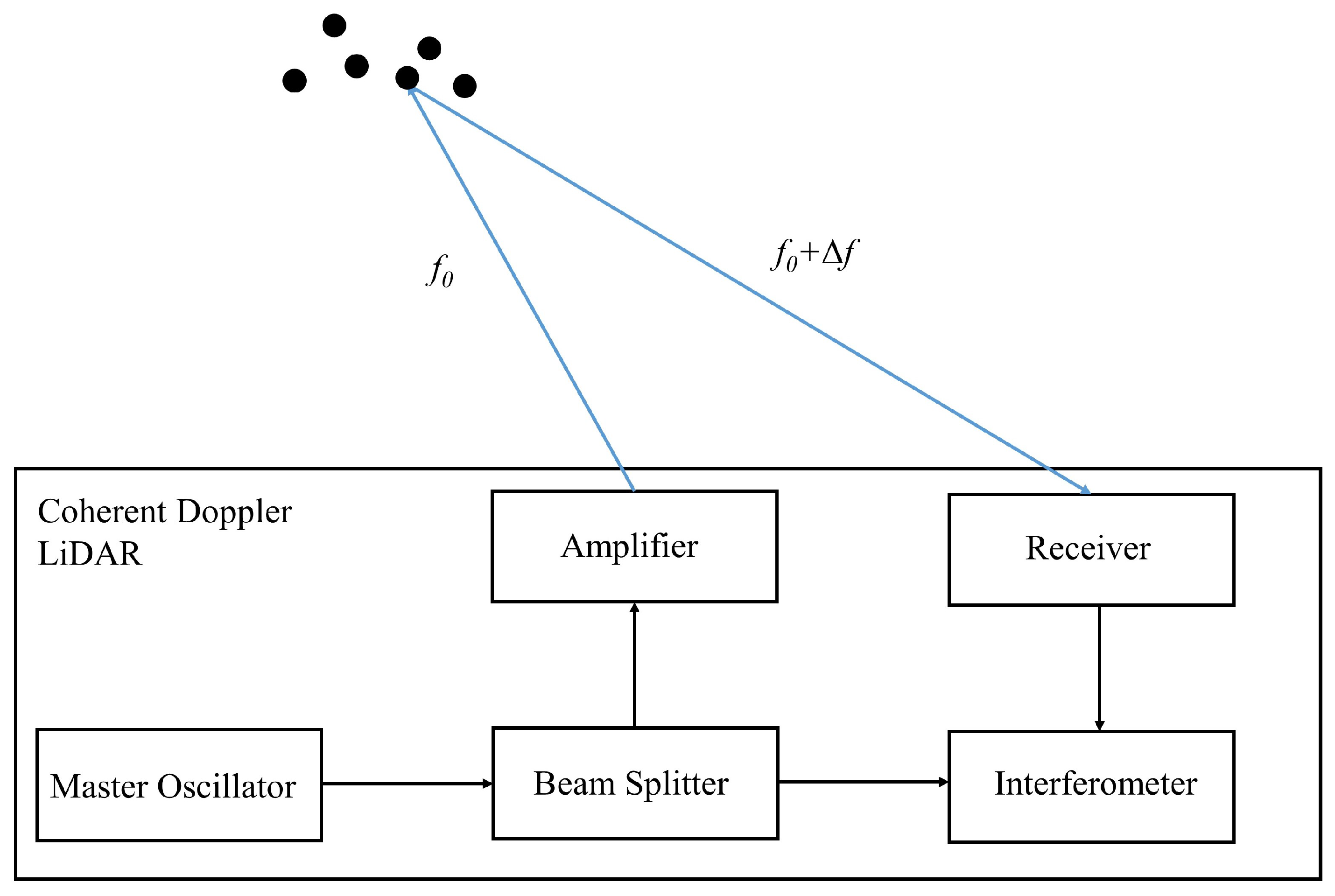
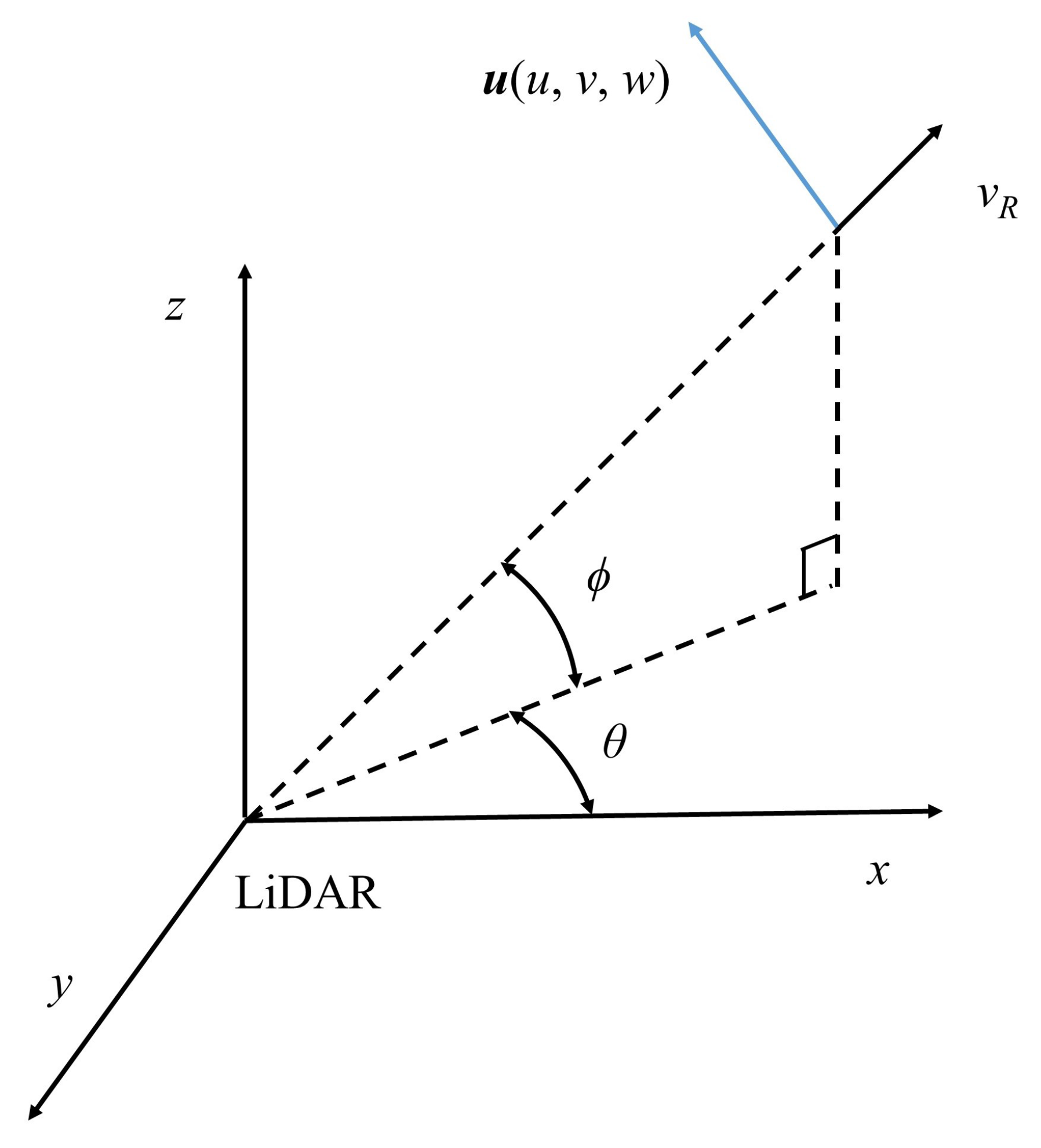
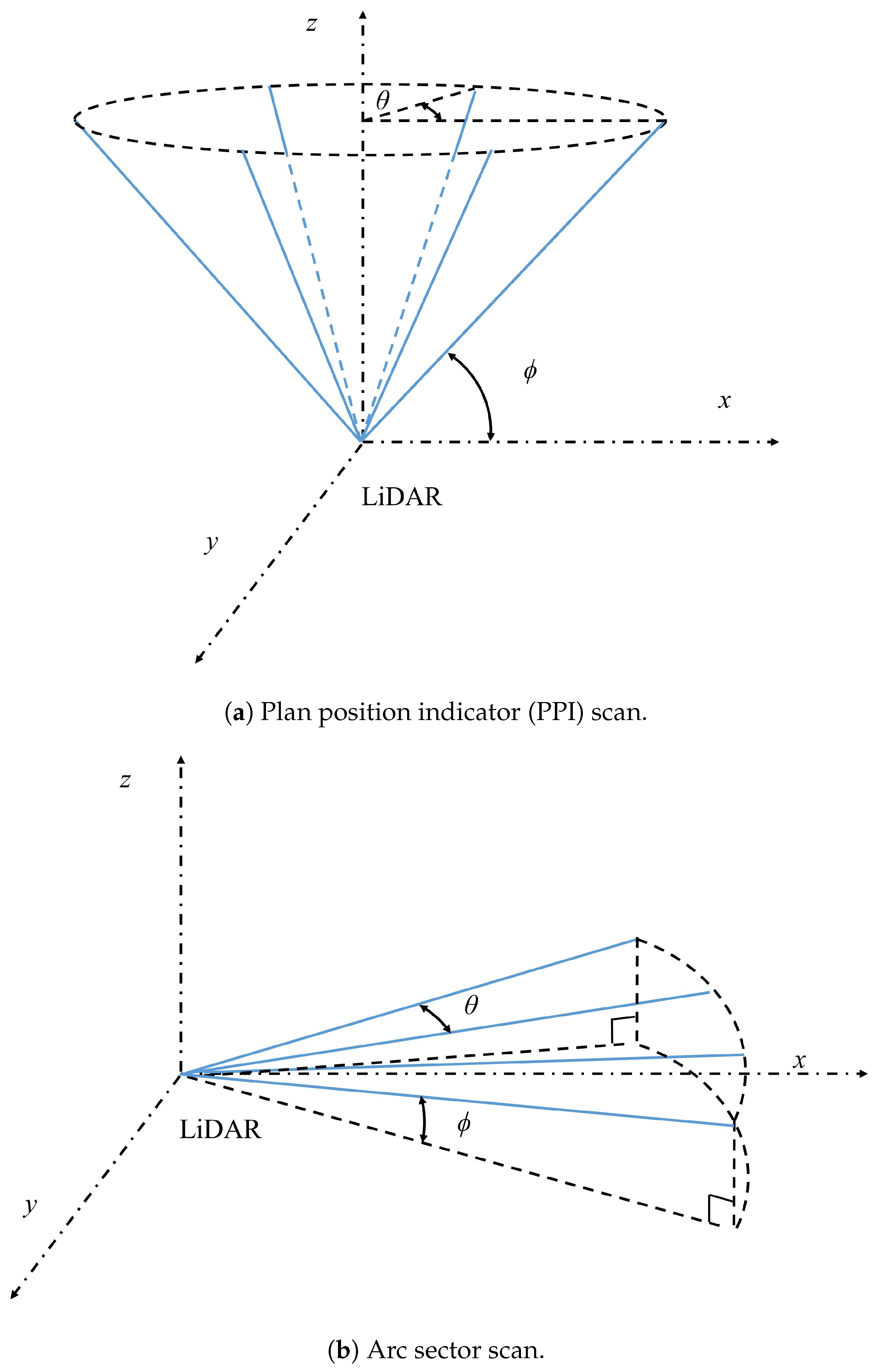
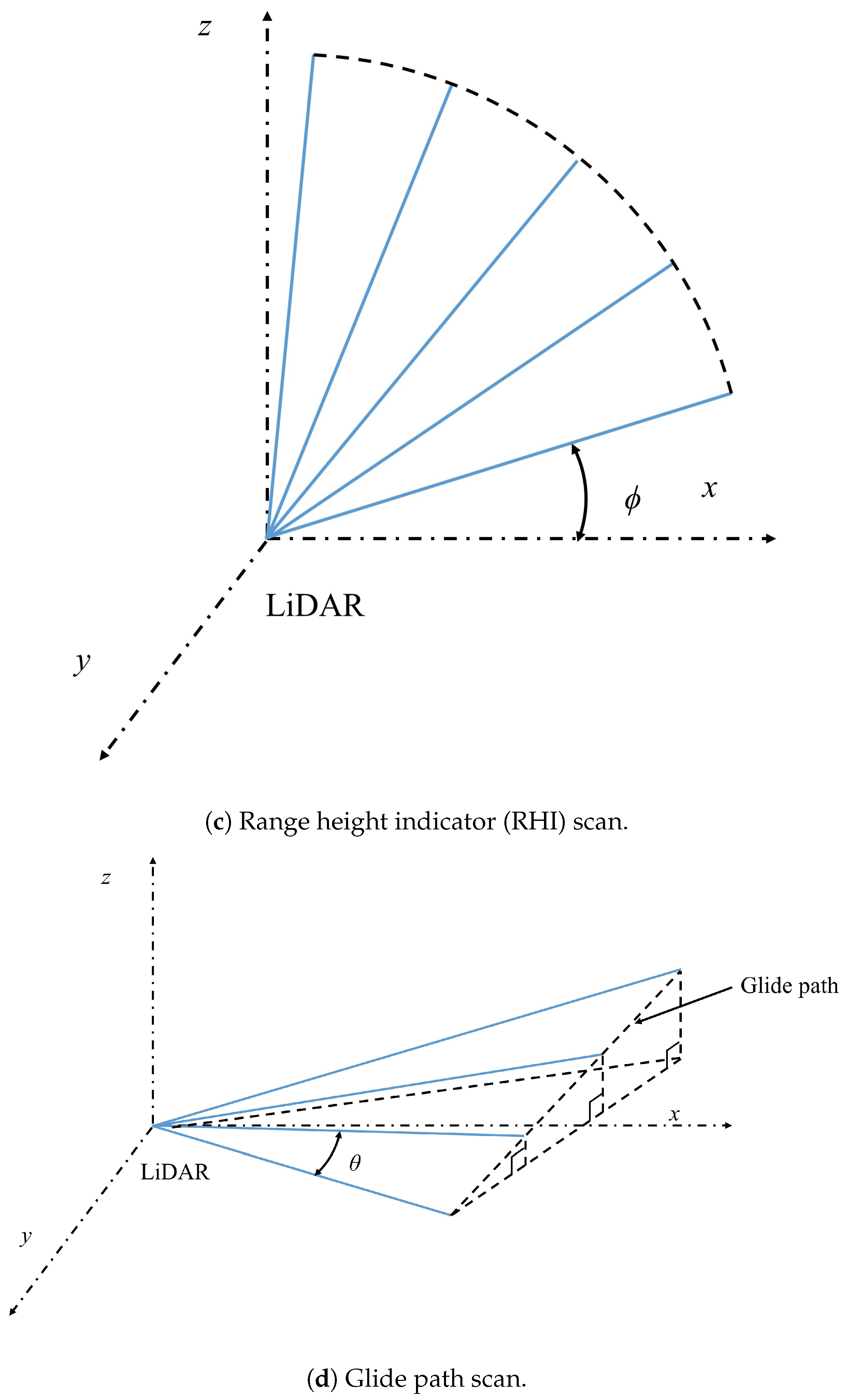
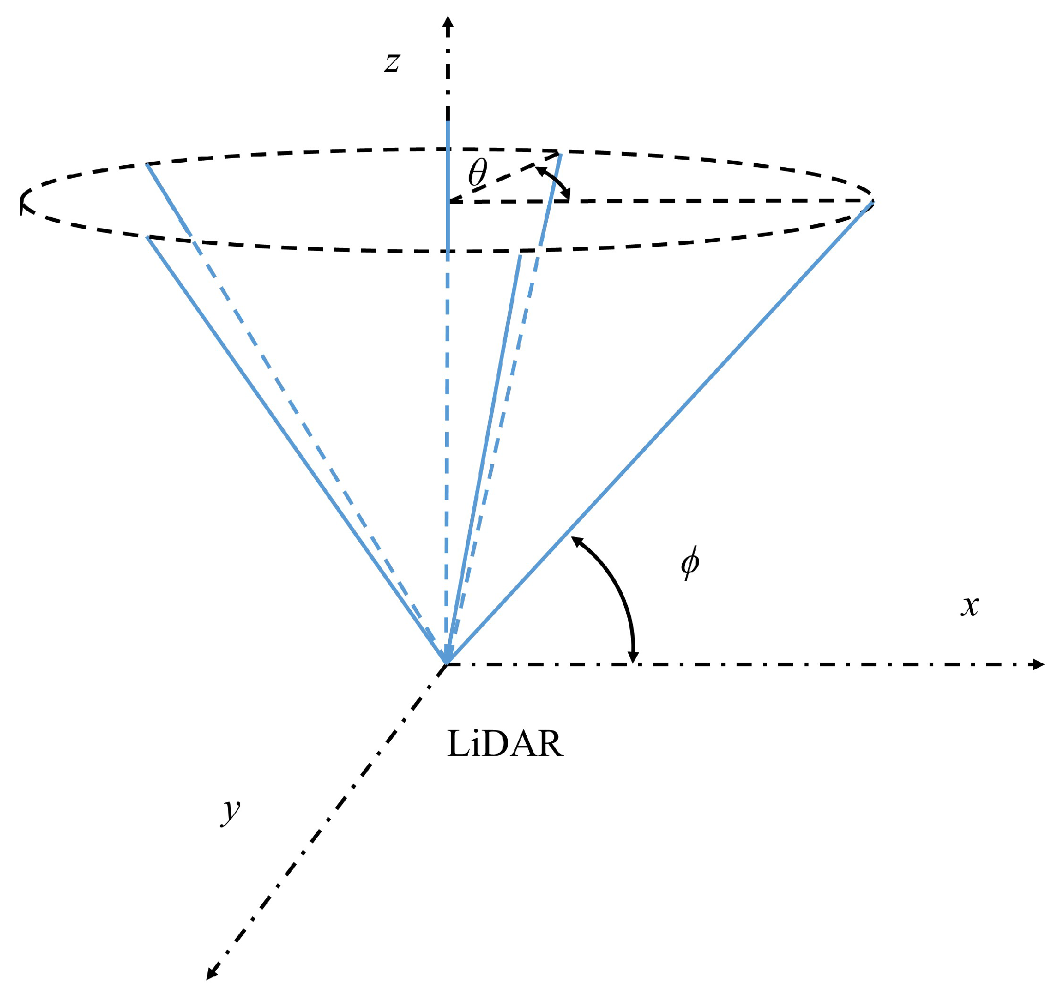
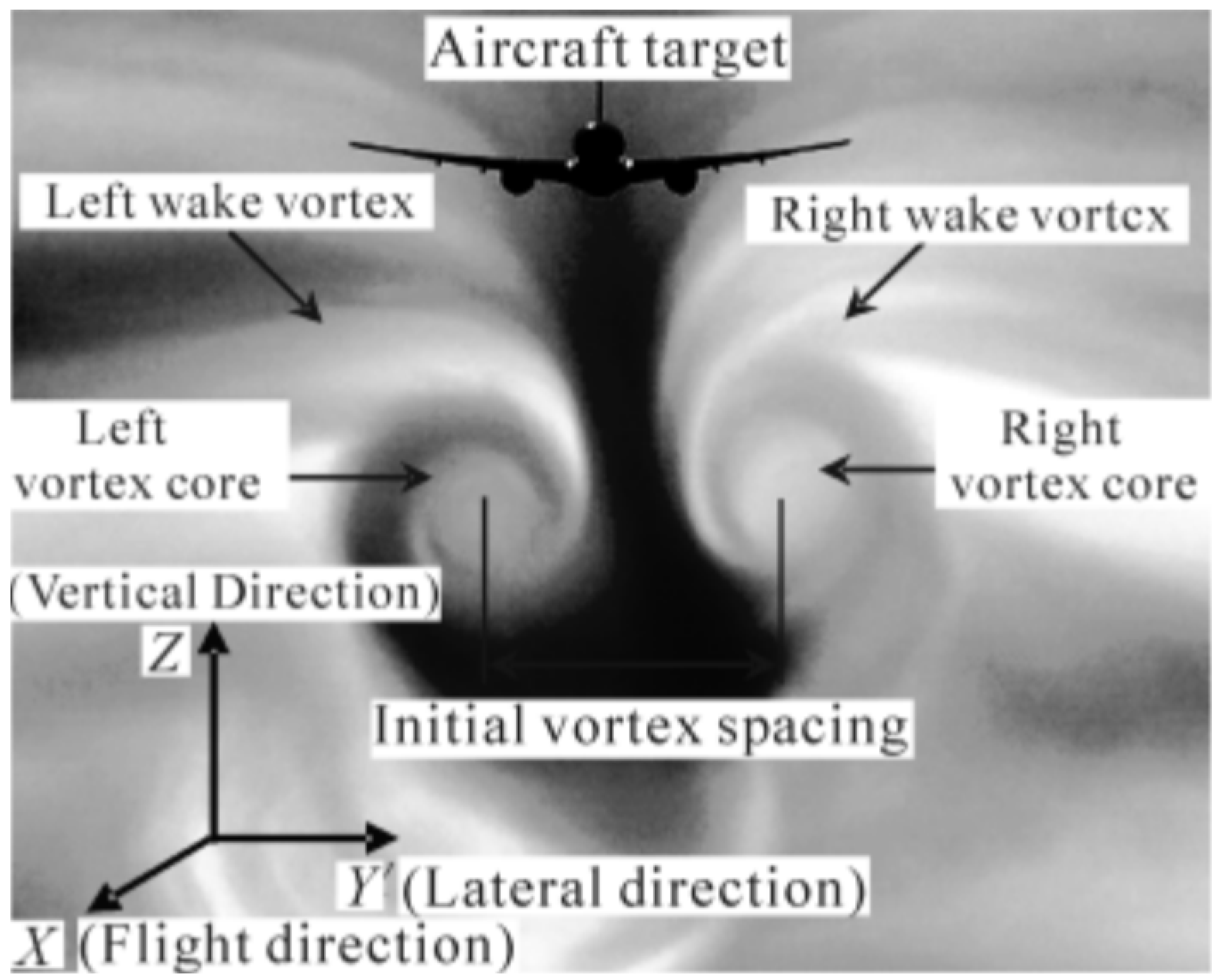
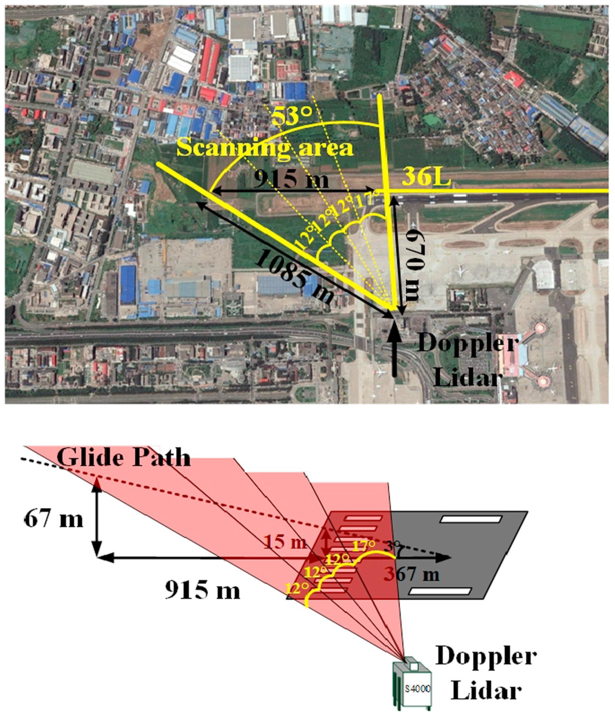
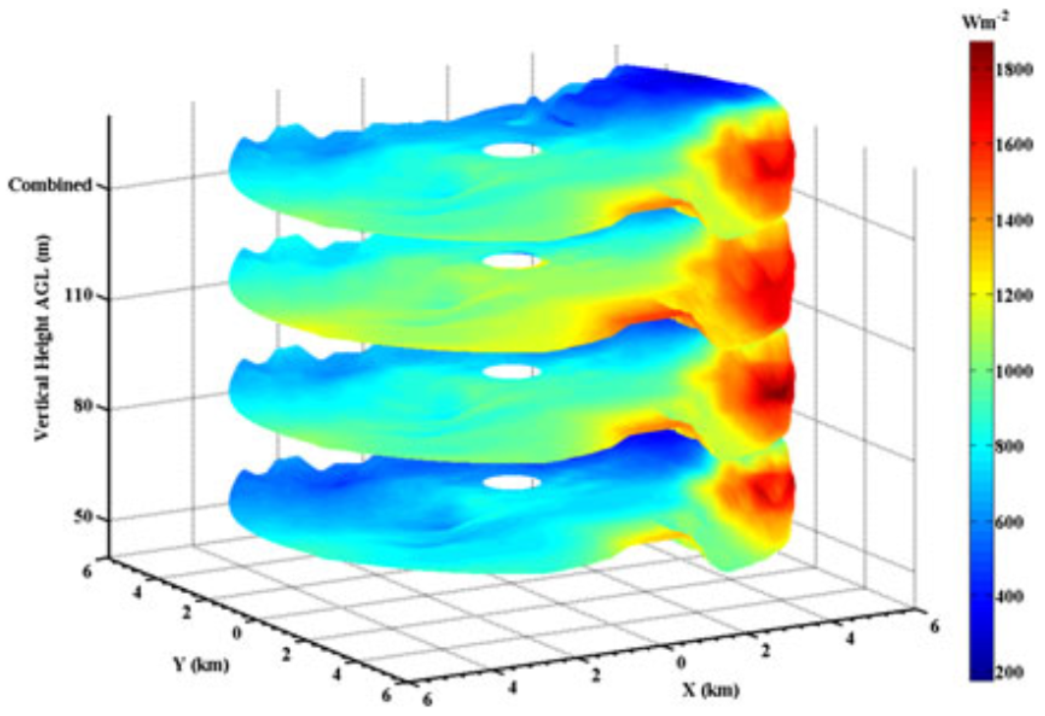
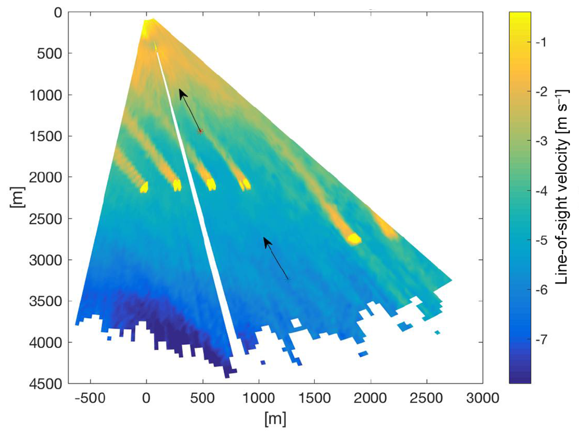
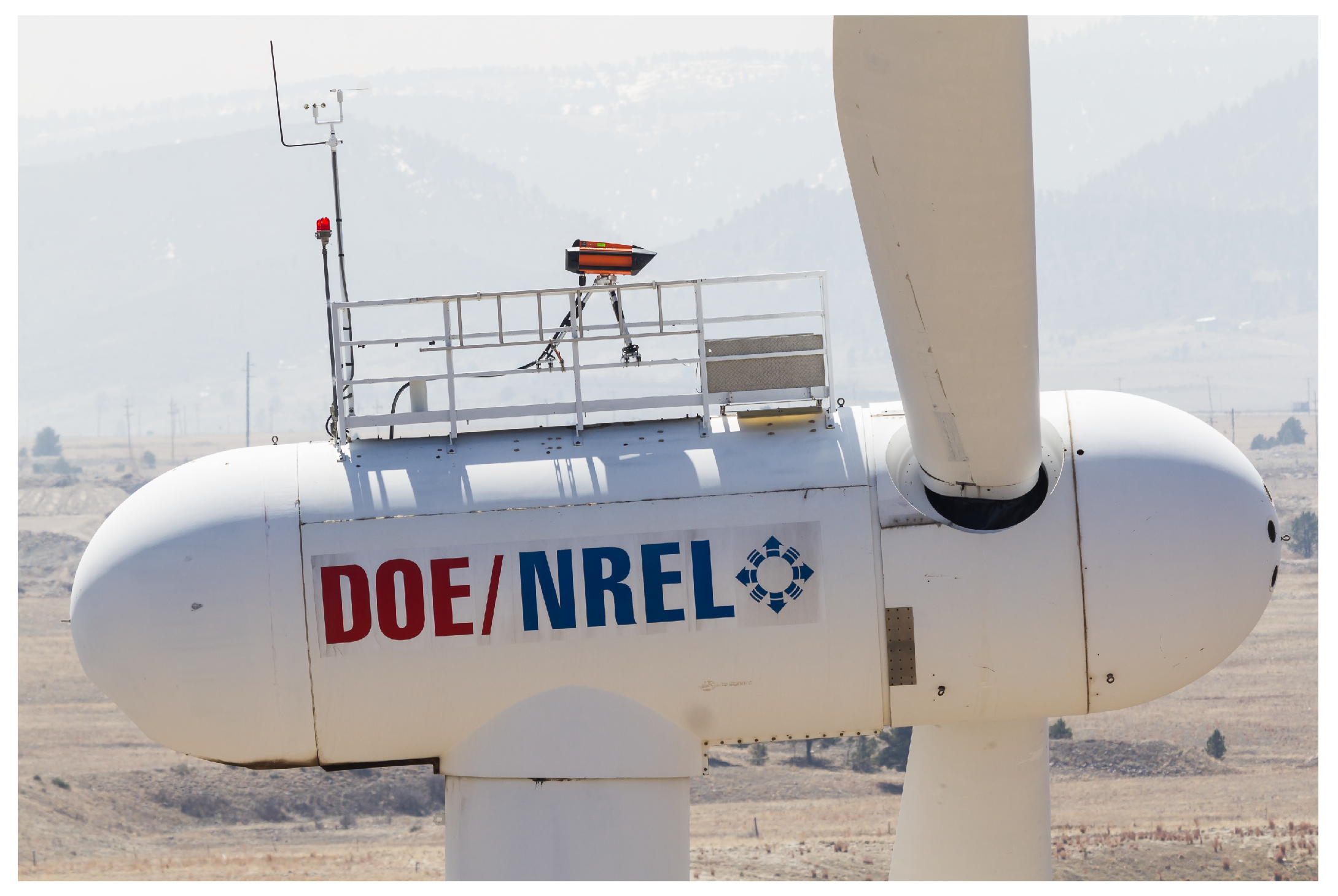
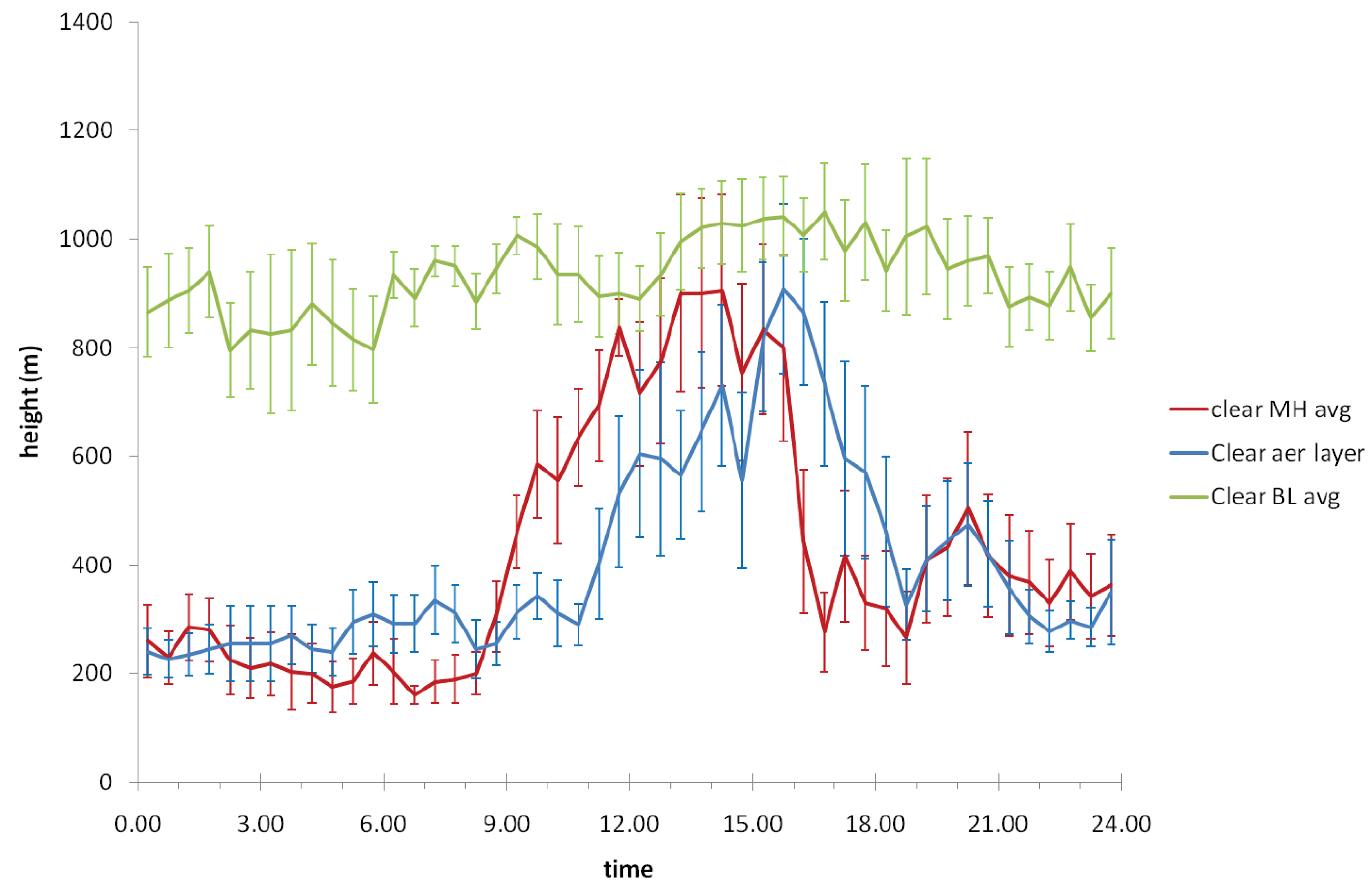
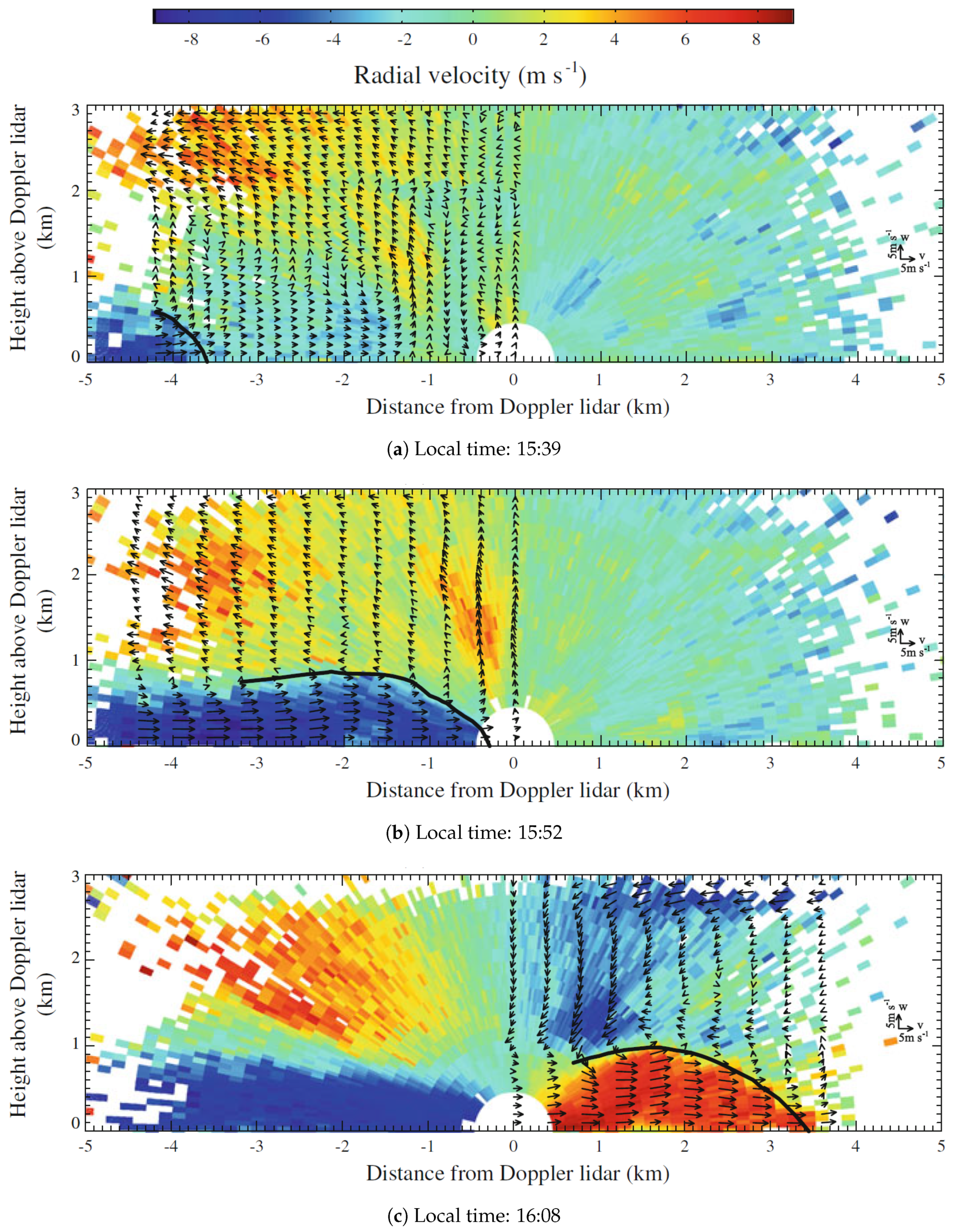
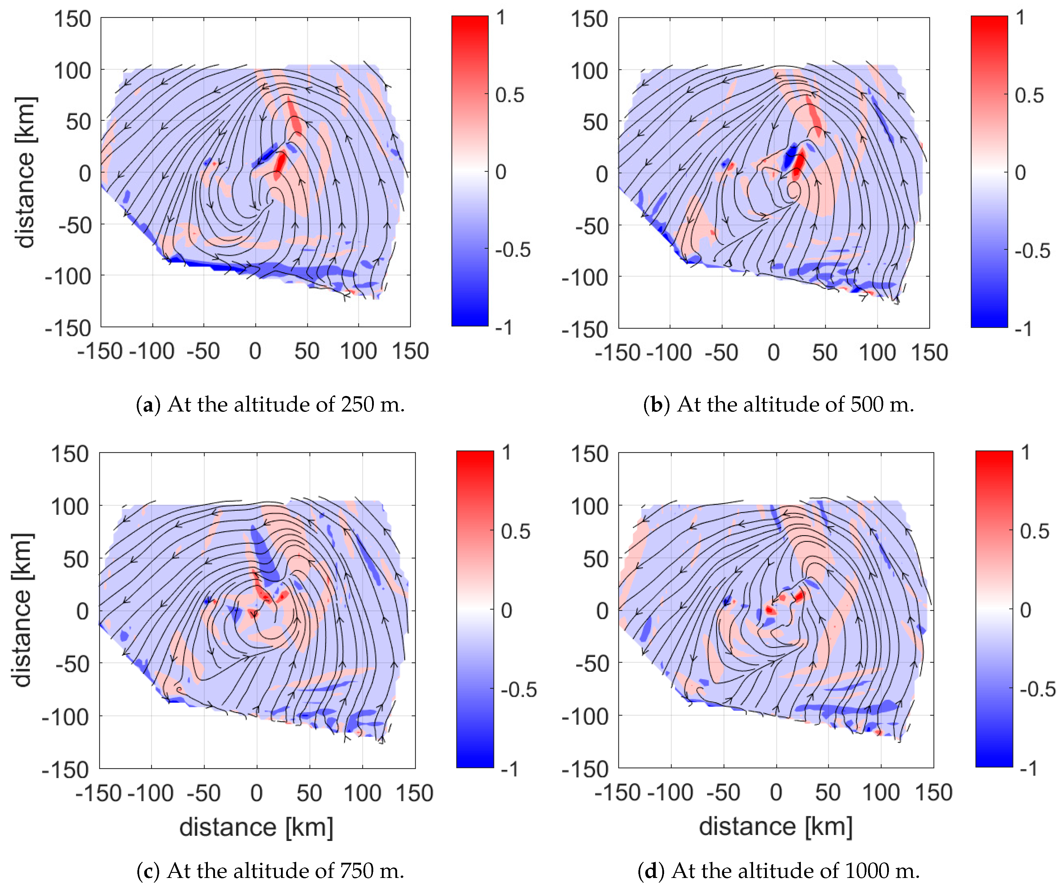
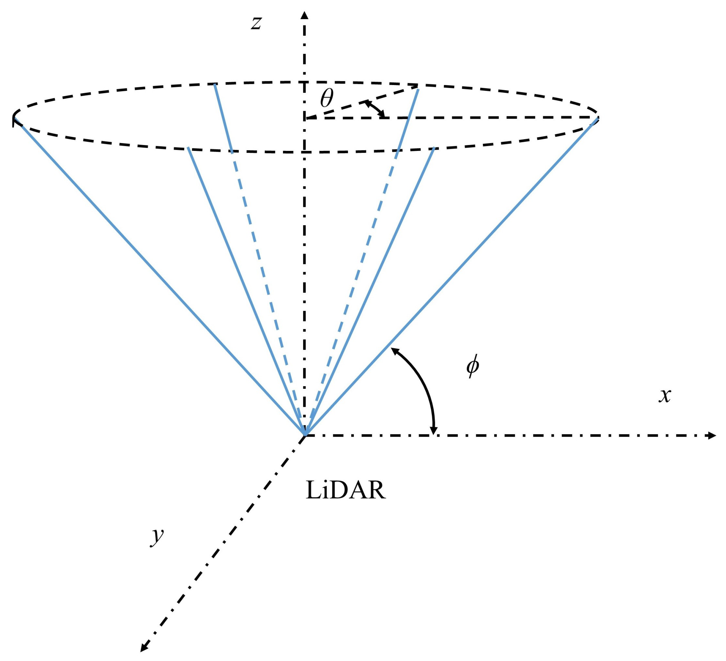
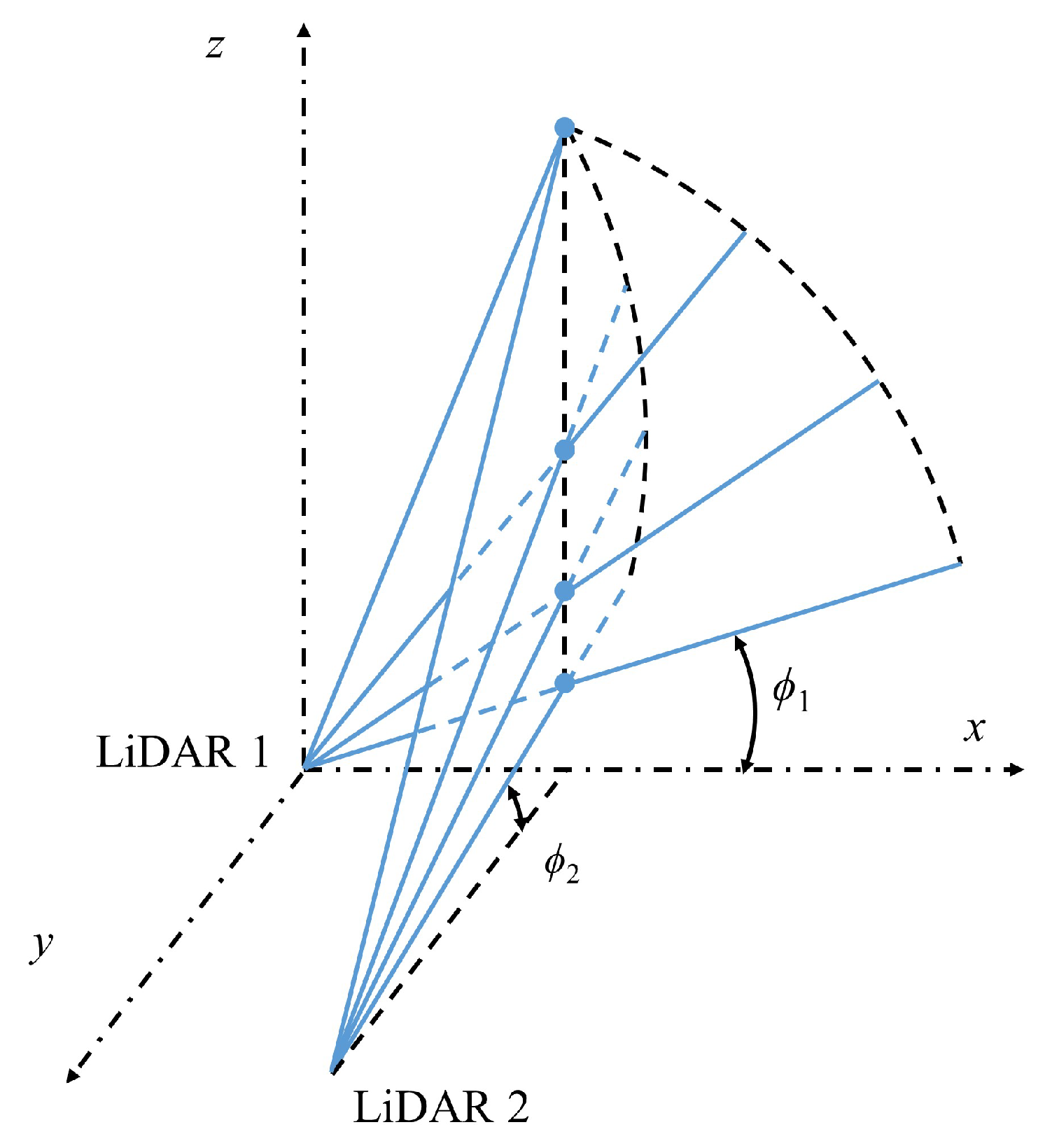
Table A1.
Literature on pulsed Doppler LiDARs. Measurements using a LiDAR system made by a Manufacturer were conducted during a certain Time period in Location with certain Scan Pattern. Instruments were used as references for validating LiDAR datasets. NA: Not Available.
Table A1.
Literature on pulsed Doppler LiDARs. Measurements using a LiDAR system made by a Manufacturer were conducted during a certain Time period in Location with certain Scan Pattern. Instruments were used as references for validating LiDAR datasets. NA: Not Available.
| Author | Location | Time | Manufacturer | Scan pattern | Instruments | Remarks |
|---|---|---|---|---|---|---|
| Chai et al. (2004) [197] | Leon | 24 Oct 1999 | NOAA | PPI | NA | 4DVAR |
| Köpp et al. (2004) [77] | Tarbes | Jun 2002 | DLR | RHI | NA | Aircraft wake vortices |
| Newsom & Banta (2004) [189] | Kansas | 25 Oct 1999 | NOAA | PPI | NA | 4DVAR |
| Collier et al. (2005) [190] | London | 23 Jul 2003 | University of Salford | PPI and RHI | NA | Dual LiDAR |
| Ishii et al. (2005) [198] | Wakkanai | 3 and 4 Sep 2002 | Lockheed Martin Coherent Technologies | PPI | Radiosondes and radar | Airborne |
| Köpp et al. (2005) [86] | Tarbes | Jun 2002 | DLR | RHI | NA | Aircraft wake vortices |
| Newsom et al. (2005) [188] | Oklahoma | 28 Jun to 31 Jul 2003 | CLR Photonics | RHI | NA | 4DVAR |
| Smalikho et al. (2005) [199] | Tarbes | 27 and 28 Aug 2003 | DLR | RHI | NA | Turbulence |
| Weissmann et al. (2005) [168] | Southern Germany | 19 Jul 2002 | DLR | PPI | Dropsonde | Airborne |
| Wulfmeyer & Janjić (2005) [41] | Pacific | 23 Jun 1999 | NOAA | Staring and PPI | Radiosonde | Shipborne, Boundary layer |
| Calhoun et al. (2006) [48] | Oklahoma | 9 Jul 2003 | Lockheed Martin Coherent Technologies | RHI | SODAR and radar | Dual LiDAR |
| Chan & Shao (2007) [93] | Hong Kong | 2002 to 2006 | NA | PPI and RHI | Anemometer and weather buoy | Two-step variational method |
| Davies et al. (2007) [42] | Northolt | 3 weeks in Jul 2003 | University of Salford | Staring | NA | Boundary layer |
| Weissmann & Cardinali (2007) [173] | north Atlantic | 14 to 28 Nov 2003 | DLR | PPI | Dropsonde | Airborne |
| Xia et al. (2007) [49] | Oklahoma | 28 Jun to 31 Jul 2003 | CLR Photonics | RHI | NA | Dual LIDAR, 4DVAR |
| Drechsel et al. (2008) [50] | Owens Valley | 14 Mar to 25 Apr 2006 | Lockheed Martin Coherent Technologies | PPI and RHI | Radiosonde and wind profiler | Dual LiDAR |
| Shun & Chan (2008) [55] | Hong Kong | 2003 to 2006 | NA | PPI, RHI and glide patch scan | Quick access recorder | Airport wind shear |
| Pearson et al. (2009) [37] | Cardington | 51 days in 2007 | Halo Photonics | PPI | Radiosonde, radar and ultrasonic anemometer | Boundary layer |
| Tucker et al. (2009)[146] | Houston | Jul 2006 | NOAA | Staring, PPI and RHI | Radiosonde | Shipborne, Boundary layer |
| Hill et al. (2010) [51] | Owens Valley | 25 Mar 2006 | Lockheed Martin Coherent Technologies | RHI | NA | Dual LiDAR |
| Käsler et al. (2010) [46] | Bremerhaven | NA | DLR | Arc sector and RHI | NA | Turbine wake |
| Pu et al. (2010) [163] | Pacific | 16 to 17 Aug 2008 | NA | NA | Dropsonde | Airborne, Typhoon |
| Barlow et al. (2011) [145] | London | 25 Oct to 13 Nov 2007 | Halo Photonics | Staring | Sonic anemometer | Turbulence |
| Iwai et al. (2011) [161] | Tokyo | 14 May to 15 Jun 2008 | NICT | PPI and RHI | Ceilometer | Sea breeze |
| Kiemle et al. (2011) [73] | Rhine valley | 30 Jul 2007 | DLR | PPI | In-situ sensors | Airborne, Complex terrain |
| Sathe et al. (2011) [200] | Høvsøre | Jan to Apr 2009 | Leosphere | PPI | Sonic anemometers | Turbulence |
| Schumann et al. (2011) [169] | Southern Germany and Iceland | 19 April to 18 May 2010 | DLR | PPI | In-situ aerosol instrumentation | Airborne, Valcano plume |
| Tang et al. (2011) [54] | Hong Kong | Apr 2008 to Feb 2009 | NA | PPI and RHI | NA | Two-step variational method |
| Aitken et al. (2012) [67] | Boulder and central Iowa | Jun to Aug 2010 | Leosphere | PPI | Ceilometer | LiDAR performance assessment |
| Koch et al. (2012) [113] | Virginia Beach | 4 Oct to 17 Oct 2011 | NA | Arc sector | In-situ anemometer | Offshore wind measurement |
| Kongara et al. (2012) [62] | Oklahoma | 28 Jun to 31 Jul 2003 | CLR Photonics | PPI | NA | Optimal interpolation method |
| Pichugina et al. (2012) [111] | New England | 9 Jul to 12 Aug 2004 | NOAA | PPI and RHI | NA | Shipborne |
| Weissmann et al. (2012) [164] | Pacific | 11 to 21 Sep 2008 | DLR | PPI | Dropsonde | Airborne, Typhoon |
| Drew et al. (2013) [155] | London | 22 May 2011 to 6 Jan 2012 | Halo Photonics | DBS | Sonic anemometer | Urban flow |
| Harvey et al. (2013) [151] | Southern England | 2009 | Halo photonics | Staring | NA | Boundary layer |
| Iungo et al. (2013) [44] | Canton de Valais | Jun to Aug 2011 | Halo Photonics | Staring, RHI | NA | Dual LiDAR, Turbine wake |
| Krishnamurthy et al. (2013) [103] | NA | Jun to Jul 2007 | Lockheed Martin Coherent Technologies | PPI | Cup anemometers and vanes | Wind farm optimization |
| Lane et al. (2013) [201] | London | 06 Jul 2010 to 11 Jan 2012 | Halo Photonics | DBS | Sonic anemometer | Urban flow |
| Rajewski et al. (2013) [122] | Central Iowa | 2010 and 2011 | Leosphere | NA | NA | Turbine wake |
| Smalikho et al. (2013) [119] | Boulder | Apr 2011 | NOAA | Arc sector and PPI | Sonic anemometer | Turbine wake |
| Aitken et al. (2014) [120] | Boulder | 5 Apr to 3 May 2011 | NOAA | Arc sector and RHI | NA | Turbine wake |
| Bluestein et al. (2014) [202] | Oklahoma, Texas Panhandle, Kansas and Colorado | May to Jun 2010 | Lockheed Martin Coherent Technologies | Arc sector | X-band Doppler radar | Truck-mounted, Tornado |
| Fuertes et al. (2014) [194] | Cabauw | Dec 2012 | Halo Photonics | Staring | Sonic anemometer | Trinal LiDAR, Turbulence |
| Iungo et al. (2014) [116] | Collonges | Jun to Oct 2012 | Halo Photonics | Staring, PPI and RHI | Sonic anemometer | Turbine wake |
| Kavaya et al. (2014) [165] | Atlantic | Aug to Sep 2010 | NA | Arc sector | Dropsonde | Airborne, Hurricane |
| Koch et al. (2014) [112] | Virginia and Maryland | 2012 and 2013 | NA | Arc sector and RHI | NA | Airborne, Offshore wind measurement |
| Schween et al. (2014)[69] | Jülich | Dec 2011 to Nov 2012 | Halo Photonics | NA | Radiosondes | Boundary layer |
| Achtert et al. (2015) [72] | Arctic | 5 Jul to 5 Oct 2014 | Halo Photonics | PPI | Radiosonde | Shipborne |
| Banta et al. (2015) [121] | Boulder | Mar to Apr 2011 | NOAA | Arc sector and RHI | NA | Turbine wake |
| Bastine et al. (2015) [127] | North Sea | NA | Leosphere | Staring | Ultrasonic anemometer | Turbine wake |
| Berg et al. (2015) [193] | Høvsøre | Jun 2013 | Technical University of Denmark | Sonic anemometers | Arc sector and RHI | Trinal LiDAR |
| Devara et al. (2015) [154] | Pune | 2009 and 2010 | Leosphere | PPI and DBS | Radiosonde | Boundary layer |
| Klaas et al. (2015) [203] | Kassel | NA | Leosphere | PPI | Cup and ultrasonic anemometers | Complex terrain |
| Newsom et al. (2015) [192] | Oklahoma | 21 Oct to 22 Nov 2010 | Halo Photonics | PPI and RHI | Sonic anemometer, wind profiler and radiosonde | Dual LiDAR |
| Päschke et al. (2015) [34] | Tauche | 2 Oct 2012 to 2 Oct 2013 | Halo Photonics | PPI | Radar and radiosonde | LiDAR performance assessment |
| Sathe et al. (2015) [56] | Høvsøre | 1 to 28 Jul 2013 | Technical University of Denmark | PPI and DBS | Cup anemometer | Turbulence |
| Smalikho et al. (2015) [79] | Tomsk | Summer 2014 | Halo Photonics | RHI | NA | Aircraft wake vortices |
| Vakkari et al. (2015) [147] | Limassol and Loviisa | 22 Aug to 15 Oct 2013 and 10 Dec 2013 to 17 Mar 2014 | Halo Photonics | PPI | NA | Boundary layer |
| Wang et al. (2015) [47] | Colorado | 15 to 25 Feb 2013 | SgurrEnergy | Arc sector | Cup and sonic anemometers and wind vanes | LiDAR performance assessment |
| Aubrun et al. (2016) [117] | Ablaincourt-Pressoir | Nov to Dec 2015 | Leosphere | Arc sector | NA | Multiple turbine wakes |
| Choukulkar et al. (2016) [63] | Lamar | 2 weeks in Sep 2003 | NOAA | PPI | NA | Prediction for power generated by a wind turbine |
| Floors et al. (2016) [106] | Denmark | Nov 2015 to Feb 2016 | Leosphere | PPI, RHI and arc sector | NA | Dual LIDAR |
| Kim et al. (2016) [101] | Jeju Island | 4 Feb to 23 Mar 2015 | Leosphere | PPI | Cup anemometer and wind vane | Influence of terrain complexity |
| Pauscher et al. (2016) [105] | Kassel | 3 Jul to 17 Aug 2014 | Leosphere | Staring and DBS | Sonic anemometer | Trinal LiDAR, Complex terrain |
| Van Dooren et al. (2016) [128] | North Sea | NA | Leosphere | Arc sector | NA | Dual LiDAR, Turbine wake |
| Wu et al. (2016) [53] | Longgang and Rudong | 2013 to 2015 | Seaglet Environmental Technology | PPI and RHI | Wind mast | Turbine wake |
| Bonin et al. (2017) [70] | Erie | 15 to 31 May 2015 | Leosphere | Staring, PPI, RHI and DBS | Sonic anemometer | Turbulence |
| Bodini et al. (2017) [118] | Central Iowa | June to September 2013 | Leosphere | Arc sector, PPI and RHI | NA | Multiple turbine wakes |
| Chen (2017) [170] | Tainan | 28 Jul 2015 | Leosphere | DBS | NA | Building wake |
| Cherukuru et al. (2017) [186] | North Sea | 31 Aug 2016 | Leosphere | PPI | Cup and vane anemometer | Two-dimensional variational data assimilation |
| Cheynet et al. (2017) [191] | Bjørnafjord | May to Jun 2016 | Technical University of Denmark | Staring and arc sector | Sonic Anemometer | Dual LiDAR |
| Huang et al. (2017) [143] | Beijing | Jun to Sep 2015 | Leosphere | DBS | Sonic anemometers and open-path gas analyzers | Boundary layer |
| Kawamoto (2017) [162] | Fukuoka | 11 Sep 2015 | Leosphere | DBS | NA | Sea breeze and urban heat island |
| Kikumoto et al. (2017) [159] | Tokyo | Sep to Dec 2013 and Apr to Jun 2014 | NA | PPI | ultrasonic anemometer | Urban flow |
| Lim et al. (2017) [158] | Tokyo | 1 Sep 2013 to 30 Jun 2014 | Leosphere | PPI | NA | Urban flow |
| Newsom et al. (2017) [204] | Oklahoma | 6 Mar to 16 Apr 2015 | Halo Photonics | PPI | Sonic anemometer | LiDAR performance assessment |
| Suomi et al. (2017) [39] | Høvsøre | 10 and 11 Oct 2015 | Leosphere | DBS | Sonic anemometer | Wind gusts |
| Thobois et al. (2017) [52] | Paris | NA | Leosphere | RHI | NA | Aircraft wake vortices |
| Vasiljević et al. (2017) [195] | Perdigão | 4 May to 29 Jun 2015 | Technical University of Denmark | Staring and RHI | NA | Trinal LiDAR |
| Zhai et al. (2017) [129] | Shandong, Jiangsu and Xinjiang | 2013 to 2015 | Seaglet Environmental Technology | PPI, arc sector and RHI | NA | Turbine wake |
| Bonin et al. (2018) [148] | Indianapolis | 2016 | Halo Photonics | Staring, PPI and RHI | NA | Boundary layer |
| Bucci et al. (2018) [71] | East Pacific | 2, 3, 8 and 9 Aug 2016 | NA | PPI | Dropsonde | Airborne, Tropical cyclones |
| Gao et al. (2018) [88] | Hong Kong | 2014 | Lockheed Martin Coherent Technologies | RHI | NA | Aircraft wake vortices |
| Gottschall et al. (2018) [108] | Southern Baltic Sea | 7 Feb to 8 Jun 2017 | Leosphere | DBS | NA | Shipborne |
| Halios & Barlow (2018) [149] | London | 2011 and 2012 | Halo Photonics | Staring and DBS | NA | Boundary layer |
| Karagali et al. (2018) [107] | Northern Denmark | Apr to Aug 2016 | Leosphere | RHI and arc sector | NA | Dual LiDAR, Complex terrain |
| Kotthaus et al. (2018) [153] | London | 21 Sep 2010 to 2 Mar 2011 | Halo Photonics | Staring, DBS and RHI | NA | Boundary layer |
| Manninen et al. (2018) [152] | Hyytiälä and Jülich | 1 May 2015 to 31 Dec 2016 | Halo Photonics | Staring, PPI and DBS | NA | Boundary layer |
| Pantillon et al. (2018) [167] | Karlsruhe | Dec 2016 to Mar 2017 | Lockheed Martin Coherent Technologies | PPI and RHI | Doppler C-band radar and instrumented tower | Extratropical cyclones |
| Risan et al. (2018) [43] | Central Norway | 13 Apr to 11 Jun 2015 | Halo Photonics | Staring | Sonic anemometer | Complex terrain |
| Sepe et al. (2018) [157] | Aversa | 9 Oct 2015 to 27 Jul 2016 | Leosphere | PPI | NA | Urban flow |
| Shimada et al. (2018) [110] | Hazaki | Oct 2015 to Dec 2016 | Leosphere | Staring | NA | Fetch effect |
| Thobois et al. (2018) [27] | Lanzhou | 9 months in 2016 | Leosphere | PPI and RHI | NA | Airport wind shear. Aircraft wake vortices |
| Wildmann et al. (2018) [196] | Central Portugal | 8 May to 14 Jun 2017 | Leosphere | PPI and RHI | Sonic anemometer | Trinal LiDAR, Turbine wake |
| Zhang et al. (2018) [166] | Atlantic | 26 August 2015 | Lockheed Martin Coherent Technologies | Arc sector | Dropsonde and Doppler radar | Airborne, Tropical cyclone |
| Fernando et al. (2019) [109] | Perdigão | 1 May to 15 Jun 2017 | NA | PPI and RHI | NA | Trinal LiDAR, Complex terrain |
| Palma et al. (2019) [205] | Perdigão | 2017 | NA | RHI | NA | Complex terrain |
| Wu et al. (2019) [75] | Beijing | 2017 | QINGDAO Leice Transient Technology | RHI | NA | Aircraft wake vortices |
| Yoshino (2019) [97] | Narita | 20 Jun 2012 | NA | PPI and RHI | NA | Airport wind shear |
| Zhang et al. (2019) [91] | Beijing | 2015 and 2016 | NA | Arc sector, RHI and DBS | NA | Airport wind shear |
1 National Oceanic and Atmospheric Administration (NOAA); 2 Plan position indicator; 3 Four-dimensional variational data assimilation; 4 Deutsches Zentrum für Luft- und Raumfahrt; 5 Range height indicator; 6 National Institute of Information and Communications Technology; 7 Doppler beam swinging.
References
- Laughton, J.K. Historical sketch of anemometry and anemometers. Q. J. R. Meteorol. Soc. 1882, 8, 161–189. [Google Scholar] [CrossRef]
- Kapp, S. Lidar-Based Reconstruction of Wind Fields and Application for Wind Turbine Control. Ph.D. Thesis, Carl von Ossietzky Universität Oldenburg, Oldenburg, Germany, 2017. [Google Scholar]
- Pardyjak, E.R.; Stoll, R. Improving measurement technology for the design of sustainable cities. Meas. Sci. Technol. 2017, 28, 092001. [Google Scholar] [CrossRef]
- Cuerva, A.; Sanz-Andrés, A. On sonic anemometer measurement theory. J. Wind Eng. Ind. Aerodyn. 2000, 88, 25–55. [Google Scholar] [CrossRef] [Green Version]
- Horst, T.; Semmer, S.; Maclean, G. Correction of a non-orthogonal, three-component sonic anemometer for flow distortion by transducer shadowing. Bound.-Layer Meteorol. 2015, 155, 371–395. [Google Scholar] [CrossRef]
- McKeon, B.; Comte-Bellot, G.; Foss, J.; Westerweel, J.; Scarano, F.; Tropea, C.; Meyers, J.; Lee, J.; Cavone, A.; Schodl, R.; et al. Velocity, vorticity, and mach number. In Springer Handbook of Experimental Fluid Mechanics; Springer: Berlin/Heidelberg, Germany, 2007; pp. 215–471. [Google Scholar]
- Mortensen, N. Wind measurements for wind energy applications. A review. In Proceedings of the 16th British Wind Energy Association Conference, Stirling, UK, 15–17 June 1994; Mechanical Engineering Publications Limited: London, UK, 1994. [Google Scholar]
- Lang, S.; McKeogh, E. LIDAR and SODAR Measurements of Wind Speed and Direction in Upland Terrain for Wind Energy Purposes. Remote Sens. 2011, 3, 1871–1901. [Google Scholar] [CrossRef] [Green Version]
- Crescenti, G.H. The degradation of doppler sodar performance due to noise: A review. Atmos. Environ. 1998, 32, 1499–1509. [Google Scholar] [CrossRef]
- Fujii, T.; Fukuchi, T. Laser Remote Sensing; Optical Science and Engineering; CRC Press: Boca Raton, FL, USA, 2005. [Google Scholar]
- Emeis, S.; Harris, M.; Banta, R.M. Boundary-layer anemometry by optical remote sensing for wind energy applications. Meteorol. Z. 2007, 16, 337–347. [Google Scholar] [CrossRef] [Green Version]
- Lindelöw, P. Fiber Based Coherent Lidars for Remote Wind Sensing. Ph.D. Thesis, Department of Electrical Engineering, Technical University of Denmark, Lyngby, Denmark, 2008. [Google Scholar]
- Pitter, M.; Slinger, C.; Harris, M. Introduction to continuous-wave Doppler lidar. In Chapter 4 in Remote Sensing for Wind Energy; Technical Report, DTU Wind Energy-E-Report-0029(EN); DTU Wind Energy: Roskilde, Denmark, 2013. [Google Scholar]
- Weitkamp, C. Lidar: Range-Resolved Optical Remote Sensing of the Atmosphere; Springer Science & Business: New York, NY, USA, 2006; Volume 102. [Google Scholar]
- Muñoz Porcar, C. Analysis and Design of an Edge-Technique-Based Doppler Wind Lidar: Practical Assessment of a Laboratory Prototype. Ph.D. Thesis, Departament de Teoria del Senyal i Comunicacions, Universitat Politècnica de Catalunya, Barcelona, Spain, 2013. [Google Scholar]
- Skinner, W.R.; Hays, P.B. A Comparative Study of Coherent & Incoherent Doppler Lidar Techniques; Technical Report; Marshall Space Flight Center: Huntsville, AL, USA, 1994.
- Karlsson, C.J.; Olsson, F.Å.A.; Letalick, D.; Harris, M. All-fiber multifunction continuous-wave coherent laser radar at 1.55 µm for range, speed, vibration, and wind measurements. Appl. Opt. 2000, 39, 3716–3726. [Google Scholar] [CrossRef] [PubMed]
- Rodrigo, P.J.; Pedersen, C. Field performance of an all-semiconductor laser coherent Doppler lidar. Opt. Lett. 2012, 37, 2277–2279. [Google Scholar] [CrossRef]
- Banakh, V.; Smalikho, I. Coherent Doppler Wind Lidars in a Turbulent Atmosphere; Artech House: Norwood, MA, USA, 2013. [Google Scholar]
- Cariou, J.P.; Sauvage, L.; Thobois, L.; Gorju, G.; Machta, M.; Lea, G.; Duboué, M. Long range scanning pulsed Coherent Lidar for real time wind monitoring in the Planetary Boundary Layer. In Proceedings of the 16th Conference on Coherent Laser Radar, Long Beach, CA, USA, 20–24 June 2011. [Google Scholar]
- Harris, M.; Hand, M.; Wright, A. Lidar for Turbine Control; Report No. NREL/TP-500-39154; National Renewable Energy Laboratory: Golden, CO, USA, 2006.
- Richmond, R.D.; Cain, S.C. Introduction to LADAR Systems. In Direct-Detection LADAR Systems; SPIE: Bellingham, WA, USA, 2010; Chapter 1; pp. 1–8. [Google Scholar]
- Emeis, S. Surface-Based Remote Sensing of the Atmospheric Boundary Layer; Springer: Berlin/Heidelberg, Germany; New York, NY, USA; London, UK, 2010; Volume 40. [Google Scholar]
- Nicolae, D.; Talianu, C.; Nemuc, A.; Carstea, E. Benefits and drawbacks of laser remote sensing in atmospheric research. Sci. Bull. J. Politeh. Univ. Buchar. 2008, 70, 5–14. [Google Scholar]
- Bilbro, J.W.; Vaughan, W.W. Wind field measurement in the nonprecipitous regions surrounding severe storms by an airborne pulsed Doppler lidar system. Bull. Am. Meteorol. Soc. 1978, 59, 1095–1101. [Google Scholar] [CrossRef]
- Reitebuch, O. Wind lidar for atmospheric research. In Atmospheric Physics; Springer: Berlin/Heidelberg, Germany, 2012; pp. 487–507. [Google Scholar]
- Thobois, L.; Cariou, J.P.; Gultepe, I. Review of Lidar-Based Applications for Aviation Weather. Pure Appl. Geophys. 2019, 176, 1959–1976. [Google Scholar] [CrossRef]
- Kameyama, S.; Ando, T.; Asaka, K.; Hirano, Y.; Wadaka, S. Performance of Discrete-Fourier-Transform-Based Velocity Estimators for a Wind-Sensing Coherent Doppler Lidar System in the Kolmogorov Turbulence Regime. IEEE Trans. Geosci. Remote Sens. 2009, 47, 3560–3569. [Google Scholar] [CrossRef]
- Wang, C.; Xia, H.; Liu, Y.; Lin, S.; Dou, X. Spatial resolution enhancement of coherent Doppler wind lidar using joint time–frequency analysis. Opt. Commun. 2018, 424, 48–53. [Google Scholar] [CrossRef]
- Peña, A.; Hasager, C. (Eds.) Remote Sensing for Wind Energy; Risø National Laboratory for Sustainable Energy, Technical University of Denmark: Copenhagen, Denmark, 2011.
- Lindelöw, P.; Courtney, M.; Parmentier, R.; Cariou, J.P. Wind shear proportional errors in the horizontal wind speed sensed by focused, range gated lidars. IOP Conf. Ser. Earth Environ. Sci. 2008, 1, 012023. [Google Scholar] [CrossRef]
- Lindelöw-Marsden, P. UpWind D1. Uncertainties in Wind Assessment with LIDAR; Technical Report, Risø-R-1681(EN); Risø National Laboratory (Den.), Technical University of Denmark: Roskilde, Denmark, 2009.
- Frehlich, R.G.; Yadlowsky, M.J. Performance of Mean-Frequency Estimators for Doppler Radar and Lidar. J. Atmos. Ocean. Technol. 1994, 11, 1217–1230. [Google Scholar] [CrossRef] [Green Version]
- Päschke, E.; Leinweber, R.; Lehmann, V. An assessment of the performance of a 1.5 μm Doppler lidar for operational vertical wind profiling based on a 1-year trial. Atmos. Meas. Tech. 2015, 8, 2251–2266. [Google Scholar] [CrossRef]
- Gryning, S.E.; Floors, R.; Peña, A.; Batchvarova, E.; Brümmer, B. Weibull Wind-Speed Distribution Parameters Derived from a Combination of Wind-Lidar and Tall-Mast Measurements Over Land, Coastal and Marine Sites. Bound.-Layer Meteorol. 2016, 159, 329–348. [Google Scholar] [CrossRef]
- Rye, B.J.; Hardesty, R.M. Discrete spectral peak estimation in incoherent backscatter heterodyne lidar. I. Spectral accumulation and the Cramer-Rao lower bound. IEEE Trans. Geosci. Remote Sens. 1993, 31, 16–27. [Google Scholar] [CrossRef]
- Pearson, G.; Davies, F.; Collier, C. An Analysis of the Performance of the UFAM Pulsed Doppler Lidar for Observing the Boundary Layer. J. Atmos. Ocean. Technol. 2009, 26, 240–250. [Google Scholar] [CrossRef]
- O’Connor, E.J.; Illingworth, A.J.; Brooks, I.M.; Westbrook, C.D.; Hogan, R.J.; Davies, F.; Brooks, B.J. A method for estimating the turbulent kinetic energy dissipation rate from a vertically pointing Doppler lidar, and independent evaluation from balloon-borne in situ measurements. J. Atmos. Ocean. Technol. 2010, 27, 1652–1664. [Google Scholar] [CrossRef]
- Suomi, I.; Gryning, S.E.; O’Connor, E.J.; Vihma, T. Methodology for obtaining wind gusts using Doppler lidar. Q. J. R. Meteorol. Soc. 2017, 143, 2061–2072. [Google Scholar] [CrossRef] [Green Version]
- Clifton, A.; Boquet, M.; Burin Des Roziers, E.; Westerhellweg, A.; Hofsass, M.; Klaas, T.; Vogstad, K.; Clive, P.; Harris, M.; Wylie, S.; et al. Remote Sensing of Complex Flows by Doppler Wind Lidar: Issues and Preliminary Recommendations; Technical Report; National Renewable Energy Lab. (NREL): Golden, CO, USA, 2015.
- Wulfmeyer, V.; Janjić, T. Twenty-Four-Hour Observations of the Marine Boundary Layer Using Shipborne NOAA High-Resolution Doppler Lidar. J. Appl. Meteorol. 2005, 44, 1723–1744. [Google Scholar] [CrossRef] [Green Version]
- Davies, F.; Middleton, D.; Bozier, K. Urban air pollution modelling and measurements of boundary layer height. Atmos. Environ. 2007, 41, 4040–4049. [Google Scholar] [CrossRef]
- Risan, A.; Lund, J.A.; Chang, C.Y.; Sætran, L. Wind in Complex Terrain—Lidar Measurements for Evaluation of CFD Simulations. Remote Sens. 2018, 10, 59. [Google Scholar] [CrossRef]
- Iungo, G.V.; Wu, Y.T.; Porté-Agel, F. Field Measurements of Wind Turbine Wakes with Lidars. J. Atmos. Ocean. Technol. 2013, 30, 274–287. [Google Scholar] [CrossRef] [Green Version]
- Banakh, V.A.; Smalikho, I.N.; Köpp, F.; Werner, C. Representativeness of wind measurements with a cw Doppler lidar inthe atmospheric boundary layer. Appl. Opt. 1995, 34, 2055–2067. [Google Scholar] [CrossRef]
- Käsler, Y.; Rahm, S.; Simmet, R.; Kühn, M. Wake Measurements of a Multi-MW Wind Turbine with Coherent Long-Range Pulsed Doppler Wind Lidar. J. Atmos. Ocean. Technol. 2010, 27, 1529–1532. [Google Scholar] [CrossRef] [Green Version]
- Wang, H.; Barthelmie, R.J.; Clifton, A.; Pryor, S.C. Wind Measurements from Arc Scans with Doppler Wind Lidar. J. Atmos. Ocean. Technol. 2015, 32, 2024–2040. [Google Scholar] [CrossRef]
- Calhoun, R.; Heap, R.; Princevac, M.; Newsom, R.; Fernando, H.; Ligon, D. Virtual Towers Using Coherent Doppler Lidar during the Joint Urban 2003 Dispersion Experiment. J. Appl. Meteorol. Climatol. 2006, 45, 1116–1126. [Google Scholar] [CrossRef]
- Xia, Q.; Lin, C.L.; Calhoun, R.; Newsom, R.K. Retrieval of Urban Boundary Layer Structures from Doppler Lidar Data. Part I: Accuracy Assessment. J. Atmos. Sci. 2008, 65, 3–20. [Google Scholar] [CrossRef]
- Drechsel, S.; Mayr, G.J.; Chong, M.; Weissmann, M.; Dörnbrack, A.; Calhoun, R. Three-Dimensional Wind Retrieval: Application of MUSCAT to Dual-Doppler Lidar. J. Atmos. Ocean. Technol. 2009, 26, 635–646. [Google Scholar] [CrossRef] [Green Version]
- Hill, M.; Calhoun, R.; Fernando, H.J.S.; Wieser, A.; Dörnbrack, A.; Weissmann, M.; Mayr, G.; Newsom, R. Coplanar Doppler Lidar Retrieval of Rotors from T-REX. J. Atmos. Sci. 2010, 67, 713–729. [Google Scholar] [CrossRef] [Green Version]
- Thobois, L.; Cariou, J.P. Next generation scanning Lidar systems for optimizing wake turbulence separation minima. J. Radar 2017, 6, 689–698. [Google Scholar]
- Wu, S.; Liu, B.; Liu, J.; Zhai, X.; Feng, C.; Wang, G.; Zhang, H.; Yin, J.; Wang, X.; Li, R.; et al. Wind turbine wake visualization and characteristics analysis by Doppler lidar. Opt. Express 2016, 24, A762–A780. [Google Scholar] [CrossRef]
- Tang, W.; Chan, P.W.; Haller, G. Lagrangian Coherent Structure Analysis of Terminal Winds Detected by Lidar. Part I: Turbulence Structures. J. Appl. Meteorol. Climatol. 2011, 50, 325–338. [Google Scholar] [CrossRef] [Green Version]
- Shun, C.M.; Chan, P.W. Applications of an Infrared Doppler Lidar in Detection of Wind Shear. J. Atmos. Ocean. Technol. 2008, 25, 637–655. [Google Scholar] [CrossRef]
- Sathe, A.; Mann, J.; Vasiljevic, N.; Lea, G. A six-beam method to measure turbulence statistics using ground-based wind lidars. Atmos. Meas. Tech. 2015, 8, 729–740. [Google Scholar] [CrossRef] [Green Version]
- Browning, K.A.; Wexler, R. The Determination of Kinematic Properties of a Wind Field Using Doppler Radar. J. Appl. Meteorol. 1968, 7, 105–113. [Google Scholar] [CrossRef]
- Koscielny, A.J.; Doviak, R.J.; Rabin, R. Statistical Considerations in the Estimation of Divergence from Single-Doppler Radar and Application to Prestorm Boundary-Layer Observations. J. Appl. Meteorol. 1982, 21, 197–210. [Google Scholar] [CrossRef]
- Caya, D.; Zawadzki, I. VAD Analysis of Nonlinear Wind Fields. J. Atmos. Ocean. Technol. 1992, 9, 575–587. [Google Scholar] [CrossRef] [Green Version]
- Matejka, T.; Srivastava, R.C. An Improved Version of the Extended Velocity-Azimuth Display Analysis of Single-Doppler Radar Data. J. Atmos. Ocean. Technol. 1991, 8, 453–466. [Google Scholar] [CrossRef] [Green Version]
- Xu, Q.; Gong, J. Background error covariance functions for Doppler radial-wind analysis. Q. J. R. Meteorol. Soc. 2003, 129, 1703–1720. [Google Scholar] [CrossRef]
- Kongara, S.; Calhoun, R.; Choukulkar, A.; Boldi, M.O. Velocity retrieval for coherent Doppler lidar. Int. J. Remote Sens. 2012, 33, 3596–3613. [Google Scholar] [CrossRef]
- Choukulkar, A.; Pichugina, Y.; Clack, C.T.M.; Calhoun, R.; Banta, R.; Brewer, A.; Hardesty, M. A new formulation for rotor equivalent wind speed for wind resource assessment and wind power forecasting. Wind Energy 2016, 19, 1439–1452. [Google Scholar] [CrossRef]
- Pailleux, J. Data assimilation: Optimum interpolation approach/Variational approach. In Proceedings of the ECMWF Seminar “Ten Years of Medium-Range Weather Forecasting”, Shinfield Park, Reading, UK, 4–8 September 1989; Volume 1. [Google Scholar]
- Qiu, C.J.; Xu, Q. A Simple Adjoint Method of Wind Analysis for Single-Doppler Data. J. Atmos. Ocean. Technol. 1992, 9, 588–598. [Google Scholar] [CrossRef] [Green Version]
- Sun, J.; Flicker, D.W.; Lilly, D.K. Recovery of Three-Dimensional Wind and Temperature Fields from Simulated Single-Doppler Radar Data. J. Atmos. Sci. 1991, 48, 876–890. [Google Scholar] [CrossRef] [Green Version]
- Aitken, M.L.; Rhodes, M.E.; Lundquist, J.K. Performance of a Wind-Profiling Lidar in the Region of Wind Turbine Rotor Disks. J. Atmos. Ocean. Technol. 2012, 29, 347–355. [Google Scholar] [CrossRef]
- Organization, W.M. Guide to Meteorological Instruments and Methods of Observation; Secretariat of the World Meteorological Organization: Geneva, Switzerland, 2014. [Google Scholar]
- Schween, J.H.; Hirsikko, A.; Löhnert, U.; Crewell, S. Mixing-layer height retrieval with ceilometer and Doppler lidar: From case studies to long-term assessment. Atmos. Meas. Tech. 2014, 7, 3685–3704. [Google Scholar] [CrossRef]
- Bonin, T.A.; Choukulkar, A.; Brewer, W.A.; Sandberg, S.P.; Weickmann, A.M.; Pichugina, Y.L.; Banta, R.M.; Oncley, S.P.; Wolfe, D.E. Evaluation of turbulence measurement techniques from a single Doppler lidar. Atmos. Meas. Tech. 2017, 10, 3021–3039. [Google Scholar] [CrossRef] [Green Version]
- Bucci, L.R.; O’Handley, C.; Emmitt, G.D.; Zhang, J.A.; Ryan, K.; Atlas, R. Validation of an Airborne Doppler Wind Lidar in Tropical Cyclones. Sensors 2018, 18, 4288. [Google Scholar] [CrossRef] [PubMed]
- Achtert, P.; Brooks, I.M.; Brooks, B.J.; Moat, B.I.; Prytherch, J.; Persson, P.O.G.; Tjernström, M. Measurement of wind profiles by motion-stabilised ship-borne Doppler lidar. Atmos. Meas. Tech. 2015, 8, 4993–5007. [Google Scholar] [CrossRef] [Green Version]
- Kiemle, C.; Wirth, M.; Fix, A.; Rahm, S.; Corsmeier, U.; Di Girolamo, P. Latent heat flux measurements over complex terrain by airborne water vapour and wind lidars. Q. J. R. Meteorol. Soc. 2011, 137, 190–203. [Google Scholar] [CrossRef]
- Suharev, A.; Shestakov, V.; Stefanski, K. Analysis of the affecting factors on aircraft takeoff and landing ground path length. In Proceedings of the AIP Conference Proceedings, Chongqing, China, 30–31 May 2019; AIP Publishing: Melville, NY, USA, 2019; Volume 2077, p. 020056. [Google Scholar]
- Wu, S.; Zhai, X.; Liu, B. Aircraft wake vortex and turbulence measurement under near-ground effect using coherent Doppler lidar. Opt. Express 2019, 27, 1142–1163. [Google Scholar] [CrossRef]
- Wu, Y.; Hu, Y.; Xu, S.; Li, J.; Dai, D. Design of airport wake vortex monitoring system based on 1.5-μm pulsed coherent Doppler lidar. Optoelectron. Lett. 2011, 7, 298. [Google Scholar] [CrossRef]
- Köpp, F.; Rahm, S.; Smalikho, I. Characterization of Aircraft Wake Vortices by 2-μm Pulsed Doppler Lidar. J. Atmos. Ocean. Technol. 2004, 21, 194–206. [Google Scholar] [CrossRef]
- Smalikho, I.N.; Banakh, V.A. Estimation of aircraft wake vortex parameters from data measured with a 1.5-μm coherent Doppler lidar. Opt. Lett. 2015, 40, 3408–3411. [Google Scholar] [CrossRef]
- Smalikho, I.; Banakh, V.; Holzäpfel, F.; Rahm, S. Method of radial velocities for the estimation of aircraft wake vortex parameters from data measured by coherent Doppler lidar. Opt. Express 2015, 23, A1194–A1207. [Google Scholar] [CrossRef] [Green Version]
- Frehlich, R.; Sharman, R. Maximum Likelihood Estimates of Vortex Parameters from Simulated Coherent Doppler Lidar Data. J. Atmos. Ocean. Technol. 2005, 22, 117–130. [Google Scholar] [CrossRef]
- Hallermeyer, A.; Dolfi-Bouteyre, A.; Valla, M.; Le Brusquet, L.; Fleury, G.; Thobois, L.P.; Cariou, J.P.; Duponcheel, M.; Winckelmans, G. Development and assessment of a wake vortex characterization algorithm based on a hybrid LIDAR signal processing. In Proceedings of the 8th AIAA Atmospheric and Space Environments Conference, Washington, DC, USA, 13–17 June 2016; p. 3272. [Google Scholar]
- Besson, C.; Dolfi-Bouteyre, A.; Canat, G.; Cézard, N.; Augère, B.; Durecu, A.; Lombard, L.; Valla, M.; Hallermeyer, A. Doppler LIDAR Developments for Aeronautics. Aerosp. Lab J. 2016, 1–16. [Google Scholar] [CrossRef]
- Holzäpfel, F.; Dengler, K.; Gerz, T.; Schwarz, C. Prediction of Dynamic Pairwise Wake Vortex Separations for Approach and Landing; Technical Report; DLR: Bonn, Germany, 2012. [Google Scholar]
- Körner, S.; Holzäpfel, F. Assessment of the Wake-Vortex Proximity to Landing Aircraft Exploiting Field Measurements. J. Aircr. 2019, 56, 1250–1258. [Google Scholar] [CrossRef]
- Pruis, M.J.; Delisi, D.P.; Jacob, D.; Lai, D. Summary of NASA Wake and Weather Data Collection at Memphis International Airport: 2013–2015. In Proceedings of the 8th AIAA Atmospheric and Space Environments Conference, Washington, DC, USA, 13–17 June 2016; p. 3274. [Google Scholar] [CrossRef]
- Köpp, F.; Rahm, S.; Smakikho, I.; Dolfi, A.; Cariou, J.P.; Harris, M. Comparison of Wake-Vortex Parameters Measured by Pulsed and Continuous-Wave Lidars. J. Aircr. 2005, 42, 916–923. [Google Scholar] [CrossRef]
- Holzäpfel, F.; Misaka, T.; Hennemann, I. Wake-Vortex Topology, Circulation, and Turbulent Exchange Processes. In Proceedings of the AIAA Atmospheric and Space Environments Conference, Toronto, ON, Canada, 2–5 August 2010. [Google Scholar] [CrossRef]
- Gao, H.; Li, J.; Chan, P.W.; Hon, K.K.; Wang, X. Parameter-retrieval of dry-air wake vortices with a scanning Doppler Lidar. Opt. Express 2018, 26, 16377–16392. [Google Scholar] [CrossRef] [PubMed]
- Holzäpfel, F.; Stephan, A.; Heel, T.; Körner, S. Enhanced wake vortex decay in ground proximity triggered by plate lines. Aircr. Eng. Aerosp. Technol. 2016, 88, 206–214. [Google Scholar] [CrossRef]
- Hallock, J.N.; Holzäpfel, F. A review of recent wake vortex research for increasing airport capacity. Prog. Aerosp. Sci. 2018, 98, 27–36. [Google Scholar] [CrossRef]
- Zhang, H.; Wu, S.; Wang, Q.; Liu, B.; Yin, B.; Zhai, X. Airport low-level wind shear lidar observation at Beijing Capital International Airport. Infrared Phys. Technol. 2019, 96, 113–122. [Google Scholar] [CrossRef]
- Chan, P.W.; Shun, C.M.; Wu, K.C. Operational LIDAR-based system for automatic windshear alerting at the Hong Kong International Airport. In Proceedings of the 12th Conference on Aviation, Range, and Aerospace Meteorology, Atlanta, GA, USA, 28 January–2 February 2006. [Google Scholar]
- Chan, P.W.; Shao, A.M. Depiction of complex airflow near Hong Kong International Airport using a Doppler LIDAR with a two-dimensional wind retrieval technique. Meteorol. Z. 2007, 16, 491–504. [Google Scholar] [CrossRef]
- Chan, P.W.; Hon, K.K.; Shin, D.K. Combined use of headwind ramps and gradients based on LIDAR data in the alerting of low-level windshear/turbulence. Meteorol. Z. 2011, 20, 661–670. [Google Scholar] [CrossRef]
- Chan, P.W. Application of LIDAR-based F-factor in windshear alerting. Meteorol. Z. 2012, 21, 193–204. [Google Scholar] [CrossRef]
- Lee, Y.F.; Chan, P.W. LIDAR-based F-factor for wind shear alerting: Different smoothing algorithms and application to departing flights. Meteorol. Appl. 2014, 21, 86–93. [Google Scholar] [CrossRef]
- Yoshino, K. Low-Level Wind Shear Induced by Horizontal Roll Vortices at Narita International Airport, Japan. J. Meteorol. Soc. Jpn. Ser. II 2019, 97, 403–421. [Google Scholar] [CrossRef] [Green Version]
- Oude Nijhuis, A.C.P.; Thobois, L.P.; Barbaresco, F.; De Haan, S.; Dolfi-Bouteyre, A.; Kovalev, D.; Krasnov, O.A.; Vanhoenacker-Janvier, D.; Wilson, R. Wind Hazard and Turbulence Monitoring at Airports with Lidar, Radar, and Mode-S Downlinks: The UFO Project. Bull. Am. Meteorol. Soc. 2018, 99, 2275–2293. [Google Scholar] [CrossRef] [Green Version]
- Chan, P.W. Severe wind shear at Hong Kong International Airport: Climatology and case studies. Meteorol. Appl. 2017, 24, 397–403. [Google Scholar] [CrossRef]
- Wagner, R.; Antoniou, I.; Pedersen, S.M.; Courtney, M.S.; Jørgensen, H.E. The influence of the wind speed profile on wind turbine performance measurements. Wind Energy 2009, 12, 348–362. [Google Scholar] [CrossRef]
- Kim, D.; Kim, T.; Oh, G.; Huh, J.; Ko, K. A comparison of ground-based LiDAR and met mast wind measurements for wind resource assessment over various terrain conditions. J. Wind Eng. Ind. Aerodyn. 2016, 158, 109–121. [Google Scholar] [CrossRef]
- Bowen, A.J.; Mortensen, N.G. WAsP Prediction Errors Due to Site Orography; Technical Report Risø-R-995(EN); Risø National Laboratory: Roskilde, Denmark, 2004.
- Krishnamurthy, R.; Choukulkar, A.; Calhoun, R.; Fine, J.; Oliver, A.; Barr, K. Coherent Doppler lidar for wind farm characterization. Wind Energy 2013, 16, 189–206. [Google Scholar] [CrossRef]
- Mann, J.; Angelou, N.; Arnqvist, J.; Callies, D.; Cantero, E.; Arroyo, R.C.; Courtney, M.; Cuxart, J.; Dellwik, E.; Gottschall, J.; et al. Complex terrain experiments in the New European Wind Atlas. Philos. Trans. R. Soc. A Math. Phys. and Eng. Sci. 2017, 375, 20160101. [Google Scholar] [CrossRef]
- Pauscher, L.; Vasiljevic, N.; Callies, D.; Lea, G.; Mann, J.; Klaas, T.; Hieronimus, J.; Gottschall, J.; Schwesig, A.; Kühn, M.; et al. An Inter-Comparison Study of Multi-and DBS Lidar Measurements in Complex Terrain. Remote Sens. 2016, 8, 782. [Google Scholar] [CrossRef]
- Floors, R.; Peña, A.; Lea, G.; Vasiljević, N.; Simon, E.; Courtney, M. The RUNE Experiment—A Database of Remote-Sensing Observations of Near-Shore Winds. Remote Sens. 2016, 8, 884. [Google Scholar] [CrossRef]
- Karagali, I.; Mann, J.; Dellwik, E.; Vasiljević, N. New European Wind Atlas: The Østerild balconies experiment. J. Phys. Conf. Ser. 2018, 1037, 052029. [Google Scholar] [CrossRef]
- Gottschall, J.; Catalano, E.; Dörenkämper, M.; Witha, B. The NEWA Ferry Lidar Experiment: Measuring Mesoscale Winds in the Southern Baltic Sea. Remote Sens. 2018, 10, 1620. [Google Scholar] [CrossRef]
- Fernando, H.J.S.; Mann, J.; Palma, J.M.L.M.; Lundquist, J.K.; Barthelmie, R.J.; Belo-Pereira, M.; Brown, W.O.J.; Chow, F.K.; Gerz, T.; Hocut, C.M.; et al. The Perdigão: Peering into Microscale Details of Mountain Winds. Bull. Am. Meteorol. Soc. 2019, 100, 799–819. [Google Scholar] [CrossRef]
- Shimada, S.; Takeyama, Y.; Kogaki, T.; Ohsawa, T.; Nakamura, S. Investigation of the Fetch Effect Using Onshore and Offshore Vertical LiDAR Devices. Remote Sens. 2018, 10, 1408. [Google Scholar] [CrossRef]
- Pichugina, Y.L.; Banta, R.M.; Brewer, W.A.; Sandberg, S.P.; Hardesty, R.M. Doppler Lidar–Based Wind-Profile Measurement System for Offshore Wind-Energy and Other Marine Boundary Layer Applications. J. Appl. Meteorol. Climatol. 2012, 51, 327–349. [Google Scholar] [CrossRef]
- Koch, G.J.; Beyon, J.Y.; Cowen, L.J.; Kavaya, M.J.; Grant, M.S. Three-dimensional wind profiling of offshore wind energy areas with airborne Doppler lidar. J. Appl. Remote Sens. 2014, 8, 083662. [Google Scholar] [CrossRef]
- Koch, G.J.; Beyon, J.Y.; Modlin, E.A.; Petros, M.; Yu, J.; Petzar, P.J.; Woll, S.; Kavaya, M.J. Side-scan Doppler lidar for offshore wind energy applications. J. Appl. Remote Sens. 2012, 6, 063562. [Google Scholar] [CrossRef]
- Hsuan, C.Y.; Tasi, Y.S.; Ke, J.H.; Prahmana, R.A.; Chen, K.J.; Lin, T.H. Validation and measurements of floating LiDAR for nearshore wind resource assessment application. Energy Procedia 2014, 61, 1699–1702. [Google Scholar] [CrossRef]
- Clifton, A.; Smith, A.; Fields, M. Wind Plant Preconstruction Energy Estimates. Current Practice and Opportunities; Technical Report; National Renewable Energy Lab. (NREL): Golden, CO, USA, 2016.
- Iungo, G.V.; Porté-Agel, F. Volumetric Lidar Scanning of Wind Turbine Wakes under Convective and Neutral Atmospheric Stability Regimes. J. Atmos. Ocean. Technol. 2014, 31, 2035–2048. [Google Scholar] [CrossRef]
- Aubrun, S.; Garcia, E.T.; Boquet, M.; Coupiac, O.; Girard, N. Wind turbine wake tracking and its correlations with wind turbine monitoring sensors. Preliminary results. J. Phys. Conf. Ser. 2016, 753, 032003. [Google Scholar] [CrossRef] [Green Version]
- Bodini, N.; Zardi, D.; Lundquist, J.K. Three-dimensional structure of wind turbine wakes as measured by scanning lidar. Atmos. Meas. Tech. 2017, 10, 2881–2896. [Google Scholar] [CrossRef] [Green Version]
- Smalikho, I.N.; Banakh, V.A.; Pichugina, Y.L.; Brewer, W.A.; Banta, R.M.; Lundquist, J.K.; Kelley, N.D. Lidar Investigation of Atmosphere Effect on a Wind Turbine Wake. J. Atmos. Ocean. Technol. 2013, 30, 2554–2570. [Google Scholar] [CrossRef]
- Aitken, M.L.; Banta, R.M.; Pichugina, Y.L.; Lundquist, J.K. Quantifying Wind Turbine Wake Characteristics from Scanning Remote Sensor Data. J. Atmos. Ocean. Technol. 2014, 31, 765–787. [Google Scholar] [CrossRef]
- Banta, R.M.; Pichugina, Y.L.; Brewer, W.A.; Lundquist, J.K.; Kelley, N.D.; Sandberg, S.P.; Alvarez, R.J., II; Hardesty, R.M.; Weickmann, A.M. 3D Volumetric Analysis of Wind Turbine Wake Properties in the Atmosphere Using High-Resolution Doppler Lidar. J. Atmos. Ocean. Technol. 2015, 32, 904–914. [Google Scholar] [CrossRef]
- Rajewski, D.A.; Takle, E.S.; Lundquist, J.K.; Oncley, S.; Prueger, J.H.; Horst, T.W.; Rhodes, M.E.; Pfeiffer, R.; Hatfield, J.L.; Spoth, K.K.; et al. Crop Wind Energy Experiment (CWEX): Observations of Surface-Layer, Boundary Layer, and Mesoscale Interactions with a Wind Farm. Bull. Am. Meteorol. Soc. 2013, 94, 655–672. [Google Scholar] [CrossRef]
- Rhodes, M.E.; Lundquist, J.K. The Effect of Wind-Turbine Wakes on Summertime US Midwest Atmospheric Wind Profiles as Observed with Ground-Based Doppler Lidar. Bound.-Layer Meteorol. 2013, 149, 85–103. [Google Scholar] [CrossRef] [Green Version]
- Mirocha, J.D.; Rajewski, D.A.; Marjanovic, N.; Lundquist, J.K.; Kosović, B.; Draxl, C.; Churchfield, M.J. Investigating wind turbine impacts on near-wake flow using profiling lidar data and large-eddy simulations with an actuator disk model. J. Renew. Sustain. Energy 2015, 7, 043143. [Google Scholar] [CrossRef]
- Chamorro, L.P.; Porté-Agel, F. A Wind-Tunnel Investigation of Wind-Turbine Wakes: Boundary-Layer Turbulence Effects. Bound.-Layer Meteorol. 2009, 132, 129–149. [Google Scholar] [CrossRef] [Green Version]
- Wu, Y.T.; Porté-Agel, F. Large-Eddy Simulation of Wind-Turbine Wakes: Evaluation of Turbine Parametrisations. Bound.-Layer Meteorol. 2011, 138, 345–366. [Google Scholar] [CrossRef]
- Bastine, D.; Wächter, M.; Peinke, J.; Trabucchi, D.; Kühn, M. Characterizing Wake Turbulence with Staring Lidar Measurements. J. Phys. Conf. Ser. 2015, 625, 012006. [Google Scholar] [CrossRef]
- Van Dooren, M.F.; Trabucchi, D.; Kühn, M. A Methodology for the Reconstruction of 2D Horizontal Wind Fields of Wind Turbine Wakes Based on Dual-Doppler Lidar Measurements. Remote Sens. 2016, 8, 809. [Google Scholar] [CrossRef]
- Zhai, X.; Wu, S.; Liu, B. Doppler lidar investigation of wind turbine wake characteristics and atmospheric turbulence under different surface roughness. Opt. Express 2017, 25, A515–A529. [Google Scholar] [CrossRef] [PubMed]
- Pao, L.Y.; Johnson, K.E. A tutorial on the dynamics and control of wind turbines and wind farms. In Proceedings of the 2009 American Control Conference, St. Louis, MO, USA, 10–12 June 2009; IEEE: New York, NY, USA, 2009; pp. 2076–2089. [Google Scholar] [Green Version]
- Simley, E.; Fürst, H.; Haizmann, F.; Schlipf, D. Optimizing Lidars for Wind Turbine Control Applications—Results from the IEA Wind Task 32 Workshop. Remote Sens. 2018, 10, 863. [Google Scholar] [CrossRef]
- Bossanyi, E.A.; Kumar, A.; Hugues-Salas, O. Wind turbine control applications of turbine-mounted LIDAR. J. Phys. Conf. Ser. 2014, 555, 012011. [Google Scholar] [CrossRef] [Green Version]
- Mikkelsen, T.; Hansen, K.H.; Angelou, N.; Sjöholm, M.; Harris, M.; Hadley, P.; Scullion, R.; Ellis, G.; Vives, G. Lidar wind speed measurements from a rotating spinner. In Proceedings of the 2010 European Wind Energy Conference and Exhibition, Warsaw, Poland, 20–23 April 2010; European Wind Energy Association (EWEA): Brussels, Belgium, 2010. [Google Scholar]
- Schlipf, D.; Fleming, P.; Haizmann, F.; Scholbrock, A.; Hofsäß, M.; Wright, A.; Cheng, P.W. Field Testing of Feedforward Collective Pitch Control on the CART2 Using a Nacelle-Based Lidar Scanner. J. Phys. Conf. Ser. 2014, 555, 012090. [Google Scholar] [CrossRef]
- Fleming, P.A.; Scholbrock, A.K.; Jehu, A.; Davoust, S.; Osler, E.; Wright, A.D.; Clifton, A. Field-test results using a nacelle-mounted lidar for improving wind turbine power capture by reducing yaw misalignment. J. Phys. Conf. Ser. 2014, 524, 012002. [Google Scholar] [CrossRef]
- Simley, E.; Pao, L.Y.; Frehlich, R.; Jonkman, B.; Kelley, N. Analysis of light detection and ranging wind speed measurements for wind turbine control. Wind Energy 2014, 17, 413–433. [Google Scholar] [CrossRef]
- Scholbrock, A.; Fleming, P.; Schlipf, D.; Wright, A.; Johnson, K.; Wang, N. Lidar-enhanced wind turbine control: Past, present, and future. In Proceedings of the 2016 American Control Conference (ACC), Boston, MA, USA, 6–8 July 2016; pp. 1399–1406. [Google Scholar] [CrossRef]
- Schlipf, D.; Haizmann, F.; Cosack, N.; Siebers, T.; Cheng, P.W. Detection of Wind Evolution and Lidar Trajectory Optimization for Lidar-Assisted Wind Turbine Control. Meteorol. Z. 2015, 24, 565–579. [Google Scholar] [CrossRef]
- Schlipf, D.; Kapp, S.; Anger, J.; Bischoff, O.; Hofsäß, M.; Rettenmeier, A.; Kühn, M. Prospects of optimization of energy production by lidar assisted control of wind turbines. In Proceedings of the EWEA 2011 Conference, Amsterdam, The Netherlands, 29 November–1 December 2011. [Google Scholar]
- Schlipf, D.; Fleming, P.; Kapp, S.; Scholbrock, A.; Haizmann, F.; Belen, F.; Wright, A.; Cheng, P.W. Direct Speed Control using LIDAR and turbine data. In Proceedings of the 2013 American Control Conference, Washington, DC, USA, 17–19 June 2013; pp. 2208–2213. [Google Scholar] [CrossRef]
- Dunne, F.; Schlipf, D.; Pao, L.; Wright, A.; Jonkman, B.; Kelley, N.; Simley, E. Comparison of two independent lidar-based pitch control designs. In Proceedings of the 50th AIAA Aerospace Sciences Meeting Including the New Horizons Forum and Aerospace Exposition, Nashville, TE, USA, 9–12 January 2012; p. 1151. [Google Scholar] [CrossRef]
- Lolli, S.; Delaval, A.; Loth, C.; Garnier, A.; Flamant, P.H. 0.355-micrometer direct detection wind lidar under testing during a field campaign in consideration of ESA’s ADM-Aeolus mission. Atmos. Meas. Tech. 2013, 6, 3349–3358. [Google Scholar] [CrossRef]
- Huang, M.; Gao, Z.; Miao, S.; Chen, F.; LeMone, M.A.; Li, J.; Hu, F.; Wang, L. Estimate of Boundary-Layer Depth Over Beijing, China, Using Doppler Lidar Data During SURF-2015. Bound.-Layer Meteorol. 2017, 162, 503–522. [Google Scholar] [CrossRef]
- Träumner, K.; Kottmeier, C.; Corsmeier, U.; Wieser, A. Convective Boundary-Layer Entrainment: Short Review and Progress using Doppler Lidar. Bound.-Layer Meteorol. 2011, 141, 369–391. [Google Scholar] [CrossRef]
- Barlow, J.F.; Dunbar, T.; Nemitz, E.; Wood, C.R.; Gallagher, M.; Davies, F.; O’Connor, E.; Harrison, R. Boundary layer dynamics over London, UK, as observed using Doppler lidar during REPARTEE-II. Atmos. Chem. Phys. 2011, 11, 2111–2125. [Google Scholar] [CrossRef] [Green Version]
- Tucker, S.C.; Senff, C.J.; Weickmann, A.M.; Brewer, W.A.; Banta, R.M.; Sandberg, S.P.; Law, D.C.; Hardesty, R.M. Doppler Lidar Estimation of Mixing Height Using Turbulence, Shear, and Aerosol Profiles. J. Atmos. Ocean. Technol. 2009, 26, 673–688. [Google Scholar] [CrossRef]
- Vakkari, V.; O’Connor, E.J.; Nisantzi, A.; Mamouri, R.E.; Hadjimitsis, D.G. Low-level mixing height detection in coastal locations with a scanning Doppler lidar. Atmos. Meas. Tech. 2015, 8, 1875–1885. [Google Scholar] [CrossRef] [Green Version]
- Bonin, T.A.; Carroll, B.J.; Hardesty, R.M.; Brewer, W.A.; Hajny, K.; Salmon, O.E.; Shepson, P.B. Doppler Lidar Observations of the Mixing Height in Indianapolis Using an Automated Composite Fuzzy Logic Approach. J. Atmos. Ocean. Technol. 2018, 35, 473–490. [Google Scholar] [CrossRef]
- Halios, C.H.; Barlow, J.F. Observations of the Morning Development of the Urban Boundary Layer Over London, UK, Taken During the ACTUAL Project. Bound.-Layer Meteorol. 2018, 166, 395–422. [Google Scholar] [CrossRef]
- Hogan, R.J.; Grant, A.L.; Illingworth, A.J.; Pearson, G.N.; O’Connor, E.J. Vertical velocity variance and skewness in clear and cloud-topped boundary layers as revealed by Doppler lidar. Q. J. R. Meteorol. Soc. 2009, 135, 635–643. [Google Scholar] [CrossRef]
- Harvey, N.J.; Hogan, R.J.; Dacre, H.F. A method to diagnose boundary-layer type using Doppler lidar. Q. J. R. Meteorol. Soc. 2013, 139, 1681–1693. [Google Scholar] [CrossRef]
- Manninen, A.J.; Marke, T.; Tuononen, M.; O’Connor, E.J. Atmospheric Boundary Layer Classification with Doppler Lidar. J. Geophys. Res. Atmos. 2018, 123, 8172–8189. [Google Scholar] [CrossRef]
- Kotthaus, S.; Halios, C.H.; Barlow, J.F.; Grimmond, C. Volume for pollution dispersion: London’s atmospheric boundary layer during ClearfLo observed with two ground-based lidar types. Atmos. Environ. 2018, 190, 401–414. [Google Scholar] [CrossRef]
- Devara, P.C.S.; Jaya Rao, Y.; Sonbawne, S.M.; Manoj, M.G.; Dani, K.K.; Saha, S.K. First results of compact coherent Doppler wind lidar and its validation at IITM, Pune, India. Meteorol. Appl. 2015, 22, 156–164. [Google Scholar] [CrossRef]
- Drew, D.R.; Barlow, J.F.; Lane, S.E. Observations of wind speed profiles over Greater London, UK, using a Doppler lidar. J. Wind Eng. Ind. Aerodyn. 2013, 121, 98–105. [Google Scholar] [CrossRef] [Green Version]
- Kent, C.W.; Grimmond, C.; Gatey, D.; Barlow, J.F. Assessing methods to extrapolate the vertical wind-speed profile from surface observations in a city centre during strong winds. J. Wind Eng. Ind. Aerodyn. 2018, 173, 100–111. [Google Scholar] [CrossRef]
- Sepe, V.; Rizzo, F.; Ricciardelli, F.; Avossa, A. Characterization of Mean Wind Profiles and Surface Roughness Assessment from Wind LIDAR Measurements. In Proceedings of the Conference of the Italian Association for Wind Engineering, Naples, Italy, 9–12 September 2018; Springer: Cham, Switzerland, 2018; pp. 689–702. [Google Scholar]
- Lim, J.; Akashi, Y.; Ooka, R.; Kikumoto, H.; Choi, Y. A probabilistic approach to the energy-saving potential of natural ventilation: Effect of approximation method for approaching wind velocity. Build. Environ. 2017, 122, 94–104. [Google Scholar] [CrossRef]
- Kikumoto, H.; Ooka, R.; Sugawara, H.; Lim, J. Observational study of power-law approximation of wind profiles within an urban boundary layer for various wind conditions. J. Wind Eng. Ind. Aerodyn. 2017, 164, 13–21. [Google Scholar] [CrossRef]
- Wood, C.; Pauscher, L.; Ward, H.; Kotthaus, S.; Barlow, J.; Gouvea, M.; Lane, S.; Grimmond, C. Wind observations above an urban river using a new lidar technique, scintillometry and anemometry. Sci. Total Environ. 2013, 442, 527–533. [Google Scholar] [CrossRef] [Green Version]
- Iwai, H.; Murayama, Y.; Ishii, S.; Mizutani, K.; Ohno, Y.; Hashiguchi, T. Strong Updraft at a Sea-Breeze Front and Associated Vertical Transport of Near-Surface Dense Aerosol Observed by Doppler Lidar and Ceilometer. Bound.-Layer Meteorol. 2011, 141, 117. [Google Scholar] [CrossRef]
- Kawamoto, Y. Effect of Land-Use Change on the Urban Heat Island in the Fukuoka–Kitakyushu Metropolitan Area, Japan. Sustainability 2017, 9, 1521. [Google Scholar] [CrossRef]
- Pu, Z.; Zhang, L.; Emmitt, G.D. Impact of airborne Doppler wind lidar profiles on numerical simulations of a tropical cyclone. Geophys. Res. Lett. 2010, 37. [Google Scholar] [CrossRef]
- Weissmann, M.; Langland, R.H.; Cardinali, C.; Pauley, P.M.; Rahm, S. Influence of airborne Doppler wind lidar profiles near Typhoon Sinlaku on ECMWF and NOGAPS forecasts. Q. J. R. Meteorol. Soc. 2012, 138, 118–130. [Google Scholar] [CrossRef]
- Kavaya, M.J.; Beyon, J.Y.; Koch, G.J.; Petros, M.; Petzar, P.J.; Singh, U.N.; Trieu, B.C.; Yu, J. The Doppler Aerosol Wind (DAWN) Airborne, Wind-Profiling Coherent-Detection Lidar System: Overview and Preliminary Flight Results. J. Atmos. Ocean. Technol. 2014, 31, 826–842. [Google Scholar] [CrossRef]
- Zhang, J.A.; Atlas, R.; Emmitt, G.D.; Bucci, L.; Ryan, K. Airborne Doppler Wind Lidar Observations of the Tropical Cyclone Boundary Layer. Remote Sens. 2018, 10, 825. [Google Scholar] [CrossRef]
- Pantillon, F.; Wieser, A.; Adler, B.; Corsmeier, U.; Knippertz, P. Overview and first results of the Wind and Storms Experiment (WASTEX): A field campaign to observe the formation of gusts using a Doppler lidar. Adv. Sci. Res. 2018, 15, 91–97. [Google Scholar] [CrossRef]
- Weissmann, M.; Braun, F.J.; Gantner, L.; Mayr, G.J.; Rahm, S.; Reitebuch, O. The Alpine Mountain–Plain Circulation: Airborne Doppler Lidar Measurements and Numerical Simulations. Mon. Weather Rev. 2005, 133, 3095–3109. [Google Scholar] [CrossRef]
- Schumann, U.; Weinzierl, B.; Reitebuch, O.; Schlager, H.; Minikin, A.; Forster, C.; Baumann, R.; Sailer, T.; Graf, K.; Mannstein, H.; et al. Airborne observations of the Eyjafjalla volcano ash cloud over Europe during air space closure in April and May 2010. Atmos. Chem. Phys. 2011, 11, 2245–2279. [Google Scholar] [CrossRef] [Green Version]
- Chen, B.W. Comparison of Field Measurements and Numerical Simulations for Atmospheric Boundary Layer Flow over a Cylindrical Building. Master’s Thesis, National Cheng Kung University, Tainan, Taiwan, 2017. [Google Scholar]
- Baker, W.E.; Atlas, R.; Cardinali, C.; Clement, A.; Emmitt, G.D.; Gentry, B.M.; Hardesty, R.M.; Källén, E.; Kavaya, M.J.; Langland, R.; et al. Lidar-Measured Wind Profiles: The Missing Link in the Global Observing System. Bull. Am. Meteorol. Soc. 2014, 95, 543–564. [Google Scholar] [CrossRef]
- Skamarock, W.C.; Klemp, J.B.; Dudhia, J.; Gill, D.O.; Barker, D.M.; Wang, W.; Powers, J.G. A Description of the Advanced Research WRF Version 2; Technical Report; National Center for Atmospheric Research Boulder Co Mesoscale and Microscale: Boulder, CO, USA, 2005.
- Weissmann, M.; Cardinali, C. The impact of airborne Doppler lidar observations on ECMWF forecasts. ECMWF Tech. Memo. 2007, 16. [Google Scholar] [CrossRef]
- Bradley, S.; Strehz, A.; Emeis, S. Remote sensing winds in complex terrain—A review. Meteorol. Z. 2015, 24, 547–555. [Google Scholar] [CrossRef]
- Mann, J.; Menke, R.; Vasiljević, N.; Berg, J.; Troldborg, N. Challenges in using scanning lidars to estimate wind resources in complex terrain. J. Phys. Conf. Ser. 2018, 1037, 072017. [Google Scholar] [CrossRef]
- Sørensen, S.T.; Warden, M.; Macarthur, J.; Silver, M.; Holtom, T.C.; McDonald, C.; Clive, P.; Bookey, H.T. Advances in Doppler Lidar for Accurate 3D Wind Measurements. In Imaging and Applied Optics 2018 (3D, AO, AIO, COSI, DH, IS, LACSEA, LS& C, MATH, pcAOP); OSA Publishing: Washington DC, USA, 2018; p. AM2A-3. [Google Scholar]
- Oertel, S.; Eggert, M.; Gutsmuths, C.; Wilhelm, P.; Müller, H.; Többen, H. Validation of three-component wind lidar sensor for traceable highly resolved wind vector measurements. J. Sens. Sens. Syst. 2019, 8, 9–17. [Google Scholar] [CrossRef]
- Clifton, A.; Clive, P.; Gottschall, J.; Schlipf, D.; Simley, E.; Simmons, L.; Stein, D.; Trabucchi, D.; Vasiljevic, N.; Würth, I. IEA Wind Task 32: Wind Lidar Identifying and Mitigating Barriers to the Adoption of Wind Lidar. Remote Sens. 2018, 10, 406. [Google Scholar] [CrossRef]
- Sathe, A.; Mann, J. A review of turbulence measurements using ground-based wind lidars. Atmos. Meas. Tech. 2013, 6, 3147–3167. [Google Scholar] [CrossRef] [Green Version]
- Gao, J.; Droegemeier, K.K.; Gong, J.; Xu, Q. A Method for Retrieving Mean Horizontal Wind Profiles from Single-Doppler Radar Observations Contaminated by Aliasing. Mon. Weather Rev. 2004, 132, 1399–1409. [Google Scholar] [CrossRef]
- Boccippio, D.J. A Diagnostic Analysis of the VVP Single-Doppler Retrieval Technique. J. Atmos. Ocean. Technol. 1995, 12, 230–248. [Google Scholar] [CrossRef] [Green Version]
- Xu, Q.; Liu, S.; Xue, M. Background error covariance functions for vector wind analyses using Doppler-radar radial-velocity observations. Q. J. R. Meteorol. Soc. 2006, 132, 2887–2904. [Google Scholar] [CrossRef]
- Xu, Q.; Nai, K.; Wei, L. An innovation method for estimating radar radial-velocity observation error and background wind error covariances. Q. J. R. Meteorol. Soc. 2007, 133, 407–415. [Google Scholar] [CrossRef]
- Lorenc, A.C. Atmospheric Data Assimilation; Meteorological Office: Berkshire, UK, 1995.
- Choukulkar, A.; Calhoun, R.; Billings, B.; Doyle, J.D. A Modified Optimal Interpolation Technique for Vector Retrieval for Coherent Doppler LIDAR. IEEE Geosci. Remote Sens. Lett. 2012, 9, 1132–1136. [Google Scholar] [CrossRef]
- Cherukuru, N.W.; Calhoun, R.; Krishnamurthy, R.; Benny, S.; Reuder, J.; Flügge, M. 2D VAR single Doppler lidar vector retrieval and its application in offshore wind energy. Energy Procedia 2017, 137, 497–504. [Google Scholar] [CrossRef]
- Qiu, C.J.; Shao, A.M.; Liu, S.; Xu, Q. A two-step variational method for three-dimensional wind retrieval from single Doppler radar. Meteorol. Atmos. Phys. 2006, 91, 1–8. [Google Scholar] [CrossRef]
- Newsom, R.K.; Ligon, D.; Calhoun, R.; Heap, R.; Cregan, E.; Princevac, M. Retrieval of Microscale Wind and Temperature Fields from Single- and Dual-Doppler Lidar Data. J. Appl. Meteorol. 2005, 44, 1324–1345. [Google Scholar] [CrossRef]
- Newsom, R.K.; Banta, R.M. Assimilating Coherent Doppler Lidar Measurements into a Model of the Atmospheric Boundary Layer. Part I: Algorithm Development and Sensitivity to Measurement Error. J. Atmos. Ocean. Technol. 2004, 21, 1328–1345. [Google Scholar] [CrossRef]
- Collier, C.G.; Davies, F.; Bozier, K.E.; Holt, A.R.; Middleton, D.R.; Pearson, G.N.; Siemen, S.; Willetts, D.V.; Upton, G.J.G.; Young, R.I. Dual-Doppler Lidar Measurements for Improving Dispersion Models. Bull. Am. Meteorol. Soc. 2005, 86, 825–838. [Google Scholar] [CrossRef]
- Cheynet, E.; Jakobsen, J.B.; Snæbjörnsson, J.; Mann, J.; Courtney, M.; Lea, G.; Svardal, B. Measurements of Surface-Layer Turbulence in a Wide Norwegian Fjord Using Synchronized Long-Range Doppler Wind Lidars. Remote Sens. 2017, 9, 977. [Google Scholar] [CrossRef]
- Newsom, R.K.; Berg, L.K.; Shaw, W.J.; Fischer, M.L. Turbine-scale wind field measurements using dual-Doppler lidar. Wind Energy 2015, 18, 219–235. [Google Scholar] [CrossRef]
- Berg, J.; Vasiljevíc, N.; Kelly, M.; Lea, G.; Courtney, M. Addressing Spatial Variability of Surface-Layer Wind with Long-Range WindScanners. J. Atmos. Ocean. Technol. 2015, 32, 518–527. [Google Scholar] [CrossRef] [Green Version]
- Fuertes, F.C.; Iungo, G.V.; Porté-Agel, F. 3D Turbulence Measurements Using Three Synchronous Wind Lidars: Validation against Sonic Anemometry. J. Atmos. Ocean. Technol. 2014, 31, 1549–1556. [Google Scholar] [CrossRef]
- Vasiljević, N.; Palma, J.M.L.M.; Angelou, N.; Carlos Matos, J.; Menke, R.; Lea, G.; Mann, J.; Courtney, M.; Frölen Ribeiro, L.; Gomes, V.M.M.G.C. Perdigão 2015: Methodology for atmospheric multi-Doppler lidar experiments. Atmos. Meas. Tech. 2017, 10, 3463–3483. [Google Scholar] [CrossRef]
- Wildmann, N.; Vasiljevic, N.; Gerz, T. Wind turbine wake measurements with automatically adjusting scanning trajectories in a multi-Doppler lidar setup. Atmos. Meas. Tech. 2018, 11, 3801–3814. [Google Scholar] [CrossRef] [Green Version]
- Chai, T.; Lin, C.L.; Newsom, R.K. Retrieval of Microscale Flow Structures from High-Resolution Doppler Lidar Data Using an Adjoint Model. J. Atmos. Sci. 2004, 61, 1500–1520. [Google Scholar] [CrossRef]
- Ishii, S.; MizutaniI, K.; Aoki, T.; Sasano, M.; Murayama, Y.; Itabe, T.; Asai, K. Wind Profiling with an Eye-Safe Coherent Doppler Lidar System: Comparison with Radiosondes and VHF Radar. J. Meteorol. Soc. Jpn. Ser. II 2005, 83, 1041–1056. [Google Scholar] [CrossRef] [Green Version]
- Smalikho, I.; Köpp, F.; Rahm, S. Measurement of Atmospheric Turbulence by 2-μm Doppler Lidar. J. Atmos. Ocean. Technol. 2005, 22, 1733–1747. [Google Scholar] [CrossRef]
- Sathe, A.; Mann, J.; Gottschall, J.; Courtney, M.S. Can Wind Lidars Measure Turbulence? J. Atmos. Ocean. Technol. 2011, 28, 853–868. [Google Scholar] [CrossRef] [Green Version]
- Lane, S.; Barlow, J.; Wood, C. An assessment of a three-beam Doppler lidar wind profiling method for use in urban areas. J. Wind Eng. Ind. Aerodyn. 2013, 119, 53–59. [Google Scholar] [CrossRef] [Green Version]
- Bluestein, H.B.; Houser, J.B.; French, M.M.; Snyder, J.C.; Emmitt, G.D.; PopStefanija, I.; Baldi, C.; Bluth, R.T. Observations of the Boundary Layer near Tornadoes and in Supercells Using a Mobile, Collocated, Pulsed Doppler Lidar and Radar. J. Atmos. Ocean. Technol. 2014, 31, 302–325. [Google Scholar] [CrossRef] [Green Version]
- Klaas, T.; Pauscher, L.; Callies, D. LiDAR-mast deviations in complex terrain and their simulation using CFD. Meteorol. Z. 2015, 24, 591–603. [Google Scholar] [CrossRef]
- Newsom, R.K.; Brewer, W.A.; Wilczak, J.M.; Wolfe, D.; Oncley, S.; Lundquist, J.K. Validating precision estimates in horizontal wind measurements from a Doppler lidar. Atmos. Meas. Tech. 2017, 10, 1229–1240. [Google Scholar] [CrossRef] [Green Version]
- Palma, J.; Lopes, A.S.; Gomes, V.C.; Rodrigues, C.V.; Menke, R.; Vasiljević, N.; Mann, J. Unravelling the wind flow over highly complex regions through computational modeling and two-dimensional lidar scanning. J. Phys. Conf. Ser. 2019, 1222, 012006. [Google Scholar] [CrossRef]
Figure 1.
Schematic diagram of the coherent Light Detection And Ranging (LiDAR) system.

Figure 2.
Wind measurements from the coherent LiDAR system. , and represent the radial velocity, the azimuth angle, and the elevation angle respectively.
Figure 2.
Wind measurements from the coherent LiDAR system. , and represent the radial velocity, the azimuth angle, and the elevation angle respectively.

Figure 3.
Schematic diagrams of scan patterns in one degree of freedom (DOF). LiDAR is placed at the origin of the Cartesian coordinate system.
Figure 3.
Schematic diagrams of scan patterns in one degree of freedom (DOF). LiDAR is placed at the origin of the Cartesian coordinate system.


Figure 4.
Schematic diagrams of DBS scan. LiDAR is placed at the origin of the Cartesian coordinate system.
Figure 4.
Schematic diagrams of DBS scan. LiDAR is placed at the origin of the Cartesian coordinate system.

Figure 5.
Cross section of wake vortices generated by the lift producing surfaces of an aircraft [76].
Figure 5.
Cross section of wake vortices generated by the lift producing surfaces of an aircraft [76].

Figure 6.
A step-wise scan along the glide path applied to detect wind shear during aircraft landing at the Beijing Capital International Airport [91]. The elevation angles are , , and in the range of azimuth angles –, –, – and –, respectively.
Figure 6.
A step-wise scan along the glide path applied to detect wind shear during aircraft landing at the Beijing Capital International Airport [91]. The elevation angles are , , and in the range of azimuth angles –, –, – and –, respectively.

Figure 7.
Estimates of wind power density at 50 m, 80 m and 110 m above the ground level and combined power density of these three layers. X (km) and Y (km) are the distances from lidar in the respective directions [103].
Figure 7.
Estimates of wind power density at 50 m, 80 m and 110 m above the ground level and combined power density of these three layers. X (km) and Y (km) are the distances from lidar in the respective directions [103].

Figure 8.
Radial velocity measured by a Doppler LiDAR [118]. The LiDAR is located at the origin of the Cartesian coordinate system. The arrows indicate the wind direction.
Figure 8.
Radial velocity measured by a Doppler LiDAR [118]. The LiDAR is located at the origin of the Cartesian coordinate system. The arrows indicate the wind direction.

Figure 9.
The pulsed LiDAR mounted on the three-bladed Controls Advanced Research Turbine located at the National Wind Technology Centercite in Boulder, Colorado [135]. Photo credit: Lee Jay Fingersh, National Renewable Energy Laboratory (NREL).
Figure 9.
The pulsed LiDAR mounted on the three-bladed Controls Advanced Research Turbine located at the National Wind Technology Centercite in Boulder, Colorado [135]. Photo credit: Lee Jay Fingersh, National Renewable Energy Laboratory (NREL).

Figure 10.
Plot of averaged boundary layer top (BL), backscatter-derived layer height (aerosol) and velocity-derived boundary layer (MH) for the diurnal cycle in clean sky conditions [145]. The boundary layer top was defined as a layer where there was a large gradient in backscatter. Error bars show standard error.

Figure 11.
Plots of radial velocity measured by a Doppler LiDAR located at the origin of the Cartesian coordinate system [161]. Black arrows represent the retrieved velocity vectors. The thick black lines are boundaries estimated by location of the maximum gradient of the radial velocity in the azimuthal direction.

Figure 12.
Contours of relative vorticity calculated from LiDAR measurements [166]. Black lines denote the streamlines.
Figure 12.
Contours of relative vorticity calculated from LiDAR measurements [166]. Black lines denote the streamlines.

Table 1.
A brief summary of wind measurement techniques.
| Technique | Advantages | Disadvantages |
|---|---|---|
| Mechanical anemometers (e.g., cup anemometers) | Extremely robust and easy to maintain [2]. | Insufficient to measure weak and unsteady wind field [3]. |
| Sonic anemometer | High sampling frequency (e.g., 100 Hz) [4]. Able to measure 3-dimensional (3D) wind vector field [5]. Most widely used technique in turbulence measurements [3]. | Unable to measure the dissipation range of turbulence accurately [6]. Additional errors may be introduced to sonic measurements due to sensor wake effects [3]. Sensitive to temperature changes [7]. |
| Sound detection and ranging devices (SODARs) | Able to measure 3D wind vector [8]. Low sampling rate (e.g., 0.1 Hz) [2]. | Generating audible acoustic noise. Measurements may be polluted by ambient noise [9], e.g., noise from construction activities. |
| Doppler wind LiDARs | Able to measure 3D wind vector field. Maximum measurement distance up to 10 km and beyond [10]. | Ineffective under adverse weather conditions such as rainfall and fog. |
© 2019 by the authors. Licensee MDPI, Basel, Switzerland. This article is an open access article distributed under the terms and conditions of the Creative Commons Attribution (CC BY) license (http://creativecommons.org/licenses/by/4.0/).
Share and Cite
MDPI and ACS Style
Liu, Z.; Barlow, J.F.; Chan, P.-W.; Fung, J.C.H.; Li, Y.; Ren, C.; Mak, H.W.L.; Ng, E. A Review of Progress and Applications of Pulsed Doppler Wind LiDARs. Remote Sens. 2019, 11, 2522. https://doi.org/10.3390/rs11212522
AMA Style
Liu Z, Barlow JF, Chan P-W, Fung JCH, Li Y, Ren C, Mak HWL, Ng E. A Review of Progress and Applications of Pulsed Doppler Wind LiDARs. Remote Sensing. 2019; 11(21):2522. https://doi.org/10.3390/rs11212522
Chicago/Turabian StyleLiu, Zhengliang, Janet F. Barlow, Pak-Wai Chan, Jimmy Chi Hung Fung, Yuguo Li, Chao Ren, Hugo Wai Leung Mak, and Edward Ng. 2019. "A Review of Progress and Applications of Pulsed Doppler Wind LiDARs" Remote Sensing 11, no. 21: 2522. https://doi.org/10.3390/rs11212522
Note that from the first issue of 2016, this journal uses article numbers instead of page numbers. See further details here.