Article

Demonstration and Evaluation of 3D Winds Generated by Tracking Features in Moisture and Ozone Fields Derived from AIRS Sounding Retrievals

Space Science and Engineering Center (SSEC), University of Wisconsin-Madison, 1225 West Dayton St., Madison, WI 53706, USA
*
Author to whom correspondence should be addressed.
Remote Sens. 2019, 11(22), 2597; https://doi.org/10.3390/rs11222597
Submission received: 31 July 2019 / Revised: 29 October 2019 / Accepted: 3 November 2019 / Published: 6 November 2019
(This article belongs to the Special Issue Satellite-Derived Wind Observations)

Abstract

:
For more than 15 years, polar winds from the Moderate Resolution Imaging Spectroradiometer (MODIS) imagery have been generated by the National Oceanic and Atmospheric Administration (NOAA) and the Cooperative Institute for Meteorological Satellite Studies (CIMSS). These datasets are a NOAA National Environmental Satellite, Data, and Information Service (NESDIS) operational satellite product that is used at more than 10 major numerical weather prediction (NWP) centers worldwide. The MODIS polar winds product is composed of both infrared window (IR-W) and water vapor (WV) tracked features. The WV atmospheric motion vectors (AMV) yield a better spatial distribution than the IR-W since both cloud and clear-sky features can be tracked in the WV images. As the new generation polar satellite-era begins with the Suomi National Polar-orbiting Partnership (S-NPP), there is currently no WV channel on the Visible/Infrared Imager/Radiometer Suite (VIIRS), resulting in a data gap with only IR-W derived AMVs possible. This scenario presents itself as an opportunity to evaluate hyperspectral infrared moisture retrievals from consecutive overlapping satellite polar passes to extract atmospheric motion from clear-sky regions on constant (and known) pressure surfaces, i.e., estimating winds in retrieval space rather than radiance space. Perhaps most significantly, this method has the potential to provide vertical wind profiles, as opposed to the current MODIS-derived single-level AMVs. In this study, the winds technique is applied to Atmospheric Infrared Sounder (AIRS) moisture retrievals from NASA’s Aqua satellite. The resulting winds are assimilated into the Goddard Earth Observing System Model, Version 5 (GEOS-5). The results are encouraging, as the AIRS retrieval polar AMVs have a similar quality as the MODIS AMVs and exhibit a positive impact in the hemispheric Day 4.5 to 6.5 forecasts for a one-month experiment in July 2012.

Graphical Abstract

1. Introduction

The economic impact of under-forecasted weather events is not only the result of the events themselves but is also driven by our lack of preparedness. It is estimated that lapses in preparedness have cost the United States over a trillion dollars in economic losses in the last 30 years [1]. To improve our preparedness, emergency managers need more accurate subseasonal forecasts (10 days and beyond). This is a multi-faceted problem that can be reduced to several basic components: the observations, our understanding of coupled atmospheric processes, an accurate initial atmospheric state, and the forecast model.
A recognized deficiency in the global observing system is an accurate depiction of the 3D structure of the global wind field. Knowledge of the wind field is essential to our understanding of general circulation and to accurately define the atmospheric state for initialization of numerical weather prediction models. However, the 3D structure of the global wind field is generally unobserved [2]. This is evident in Figure 1, which depicts a vertical cross-section of satellite-derived winds within 5° latitude of the equator, for a six-hour period centered on 00 UTC on 10 December 2014. It is clear that the geostationary satellites are not filling a data void in wind observations—especially in the middle troposphere, where there is a propensity for few clouds. This observation is confirmed in the tropics by Dessler et al. [3] who found that the heights of tropical clouds are primarily between 12 and 17 km (100–200 hPa), and below 4 km (700 hPa). Moreover, in their observing period, 34% of the time clear sky was detected which will result in the highest yield of 3D winds and are completely void of geostationary cloud-tracked winds.
The importance and expected impact of global 3D winds in weather predictability have been identified in recent independent reports. The primary motivation is to fill in data void regions, most notably over oceanic, tropical, and polar regions. This lack of data, especially wind information, is “the number-one unmet measurement objective for improving weather forecasts” [4]. For example, hurricanes are steered by tropospheric winds and their intensity is partly determined by the vertical wind shear. Therefore, the NRC 2007 Decadal Survey recommended a 3D tropospheric wind mission, using a space-based LIDAR instrument. More recently, NASA’s 2015 workshop: Scientific Challenges and Opportunities in the NASA Weather Focus Area [5], suggested other instruments to derive 3D winds, including the use of hyperspectral infrared measurements. There are several hyperspectral instruments currently in orbit (Atmospheric Infrared Sounder (AIRS), Cross-track Infrared Sounder (CrIS), Infrared Atmospheric Sounding Interferometer (IASI)) which could be used to track features from hyperspectral retrievals, resulting in vertical profiles of winds (3D winds). Moreover, our feature-tracking algorithm applied to humidity and ozone concentrations measures the total horizontal wind: this includes the ageostrophic component that is key to understanding atmospheric dynamics. Ageostrophic circulations play a significant role in the dynamics of weather systems from the mid- and high-latitudes (e.g., synoptic scale baroclinic waves [6]) and into the tropics (e.g., low-level jets [7]). This is unlike the LIDAR instrument on the Atmospheric Dynamics Mission (ADM)-Aeolus satellite, which is a single line-of-sight (LOS) and results in only the zonal component of the wind [8].
Additionally, stratospheric circulations (and their interactions with the troposphere) are slowly varying on the order of days or weeks. Therefore, these high-altitude systems will have an impact on the skill of tropospheric subseasonal forecasts [9,10]. Since the stratosphere is relatively void of direct observations, the 3D winds product will provide needed dynamical measurements to improve longer-range global forecasts.
The derivation and application of satellite-derived cloud displacements to infer atmospheric motion has been investigated since the first weather satellites were launched in the 1960s [11]. Throughout the 1970s and early 1980s, cloud motion winds were produced from sequential geostationary satellite imagery using manually-derived techniques. In 1992, the National Oceanic and Atmospheric Administration (NOAA) began using an automated winds software package developed at the Space Science and Engineering Center (SSEC).
In the early 2000s, the Cooperative Institute for Meteorological Satellite Studies (CIMSS) and NOAA pioneered the development of deriving polar winds from NASA’s Moderate Resolution Imaging Spectroradiometer (MODIS) imagery [12], from the Terra and Aqua satellites. The MODIS polar winds product is composed of both infrared window (IR-W) and water vapor (WV) tracked features. However, the WV atmospheric motion vectors (AMVs) are only attainable at mid- and upper- tropospheric levels due to the MODIS WV atmospheric contribution function, while IR-W images also provide cloud tracers for vectors at lower levels. Despite their limited usage, the WV AMVs yield a better spatial distribution than the IR-W because both cloud and clear-sky features can be tracked in the WV images.
The new generation of polar satellites beginning with the Suomi National Polar-orbiting Partnership (S-NPP) has the Visible Infrared Imaging Radiometer Suite (VIIRS) instrument, which unlike MODIS, does not have a WV channel. Therefore, a potential data gap will result as no WV features can be tracked, resulting in only the standard IR-W derived AMVs. This scenario presents itself as an opportunity to investigate using Single Field of View (SFOV) AIRS moisture retrievals from consecutive overlapping polar passes to extract atmospheric motion from clear-sky regions on constant (and known) pressure surfaces, i.e., estimating winds in retrieval space rather than radiance space.
For this study, our winds algorithm was adapted to generate AMVs from AIRS retrievals of humidity and ozone. This results in a blended product of MODIS imager- and AIRS retrieval-derived AMV datasets. Moreover, the AIRS AMVs have been generated in real-time beginning in May 2015.
This paper is organized as follows: We provide a description of the moisture and ozone retrievals, and the tracking algorithm used to produce AMVs in Section 2. The quality of the AMVs are quantified by comparing to MODIS winds, and the impact in a data assimilation and forecast model are presented in Section 3. A discussion of the results follows in Section 4. Conclusions and a look to the future are contained in Section 5.

2. Materials and Methods

There are several software components in the generation of the 3D winds, which are described in the following sections. This includes the retrievals of humidity and ozone, image processing, and the winds algorithm, which is composed of: target selection, target height assignment, wind tracking, and quality control [13]. However, the height assignment is not necessary for AIRS retrieval winds, as the retrievals resolve to constant pressure surfaces.

2.1. Retrievals of Temperature, Humidity, and Ozone

The AIRS Standard Retrieval Product provides profiles of retrieved temperature, water vapor, and ozone. The profile vertical resolution is 28 levels between 1000 and 0.02 hPa [14]. This standard product is generated from 3 × 3 Fields of View (FOVs) of AIRS radiances [15], which results in a horizontal resolution of approximately 40 km at nadir. This is much too coarse for tracking features from successive orbits (separated by 100 min), as a one-pixel displacement corresponds to a difference in wind speed of 6.7 ms−1. Weisz et al. [16] at the Cooperative Institute for Meteorological Satellite Studies (CIMSS) have developed a single field of view (SFOV) retrieval algorithm, which retains the native horizontal resolution at 13.5 km/footprint at nadir, thereby reducing a one-pixel displacement to 2.3 ms−1. The retrievals of temperature, humidity, and ozone are at 101 pressure levels from 0.005 to 1100 hPa, however, the AMV extraction in this study is only done on 29 levels in the lower-stratosphere and mid-troposphere. Comparisons of these profiles to collocated radiosondes observations (not shown) and model analyses (Figure 2) are similar to that of the Standard Retrieval product [17]. Note that this figure shows a single example of satellite-retrieved profiles (black) of temperature and humidity as compared to the model analysis (magenta), so there are variations between the two curves. However, the temperature profiles are nearly the same and the overall trends in the humidity profile are similar in the troposphere below 300 hPa, which is where we derive the AMVs by tracking humidity features. The satellite-derived ozone concentration (not shown) was not compared to an independent measurement.
We utilize the SFOV product in our AIRS AMV generation since it provides the highest spatial resolution, which is needed by our application. The SFOV retrieval package is distributed in the Community Satellite Processing Package (CSPP) as the UW Dual-Regression (DR) retrieval algorithm [17,18,19]. The DR method is based on linear regression, but with additional steps to minimize the non-linear dependence of the solution on the measured radiance. The DR provides retrievals for every FOV (i.e., at 13.5 km spatial resolution at nadir) from AIRS, IASI, and CrIS in clear-sky and above clouds.

2.2. AIRS Image Processing

The resulting vertical profiles of SFOV retrievals of humidity and ozone are then used to create horizontally sliced swath images on constant pressure surfaces. Because of the sharp pixel-to-pixel variation in moisture and ozone images, we initially found that the cross-correlation technique in the winds software was not able to track features. Therefore, an application was developed to smooth the gradients, by increasing the resolution of the images by a factor of four using bi-linear interpolation, resulting in a resolution at the nadir of approximately 3.4 km. These swath slices are then reprojected to a polar stereographic projection at 4 km resolution. The cross-correlation technique in the winds algorithm performed much better using the smooth gradient images. We are also investigating the use of optical flow as described by Hautecoeur et al. [20].

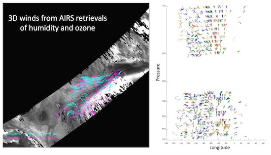
2.3. Derivation of 3D AMVs

The AIRS AMVs are extracted from a time sequence of three images. In order to achieve overlapping images, the AMVs could only be derived in high latitudes (poleward of 70° latitude). The geographic coverage of AMVs from polar orbiting satellites is over small regions at any particular time. Figure 3 illustrates the swath overlap for three consecutive passes for MODIS (Figure 3a) and AIRS (Figure 3b). Because the AIRS instrument has a narrower swath width than MODIS, the spatial coverage of the AIRS AMVs is also reduced. An entire day of successive orbit triplets is needed to get complete AMV coverage over the polar regions.
The input data files are three time-ordered humidity or ozone concentration images, each separated by one orbit (100 min), on many different pressure levels and forecast model output. Three images are used because consistency between vectors derived from each pair provides a measure of quality in the winds.
The model output is used to determine a first guess for target tracking. The 6-, 9- or 12-h forecasts are linearly interpolated to the middle-image time. From the middle image of the triplet, potential targets are determined by locating rectangular regions where the bi-directional gradient in the humidity or ozone exceeds a user-specified threshold. The target size is determined based on the spatial resolution of the images and the time interval between images. Typically, for 4 km data and 100-min time step (e.g., the Advanced Very High-Resolution Radiometer (AVHRR)), a target box size of 11 × 11 pixels is used. However, since the AIRS retrieval image is not natively 4 km (see Section 2.2), it was thought that a doubling of the target size would be more commensurate to tracking smoothed gradient features. After short-term evaluations of different target sizes, a 19 × 19 box was chosen as it resulted in the best coverage of AMVs. The search box, which is defined as the incremental increase of the target box size, is the same as for AVHRR, which is 21 pixels. Therefore, the search box size in the first and third images is 40 × 40 pixels.
Unlike tracking cloud or water vapor features in typical infrared images, tracking features in images from AIRS retrievals of humidity or ozone are in clear areas and above clouds. This results in regions that are unusable for deriving AMVs. These cloud contaminated pixels are denoted as missing and appear as black pixels in the image (see Figure 4). If even one cloud pixel is in the target or search box, the cross-correlation cannot be computed, and that potential feature to track is discarded. (Note: The reason some wind barbs appear in or near missing pixels in Figure 4 is because those AMVs are derived on other pressure levels. The underlying image is humidity at 400 hPa; the wind barbs are from all levels in both the troposphere and stratosphere.)
The initial target locations are investigated one-by-one to compute a displacement speed with the same feature at a time before and after the target image time. A first guess wind is interpolated from the model forecast at the location and pressure surface on which the features are being tracked. This guess is used to calculate a position in the first and third images of the sequence where the feature should be. The image data within the target and larger search box regions are read. A cross-correlation is computed between the target and sub-regions throughout the search box for the first pair of images. The highest correlated point between the target array within the search box is found and the vector displacement between these two points is calculated. This process is then repeated for the second image pair. Once the intermediate wind vectors are determined, acceleration checks are performed. The intermediate vectors are compared to each other. If the difference in the u- or v-component is greater than 10 ms−1, this vector is flagged as poor quality. The intermediate vectors are then compared to an interpolated model forecast wind vector. Departures greater than 10 ms−1 from the guess u- and v-components are flagged for each wind vector, although these are still considered good wind vectors. Slow vectors, speeds less than 3 ms−1, are flagged as unusable. There are two independent routines used for automatic quality control (QC) of the AMVs. The first utilizes the statistical properties of a computed quality indicator for each wind vector using several consistency tests. The Quality Indicator (QI) for each AMV is calculated by estimating consistency in the intermediate wind vector pairs, spatial coherence, and (optionally) the deviation from the model grid [21]. This second quality measure is a two-stage, three-dimensional objective analysis, based upon a recursive filter analysis, which utilizes weighted numerical model information as a background field [22]. An example of the 3D AMV spatial coverage at a single time is shown in Figure 4.

2.4. Data Assimilation and Forecast Model

In addition to comparing AIRS winds to MODIS winds, we ran three Numerical Weather Prediction (NWP) experiments to determine the overall impact on numerical forecasts and the relative contributions of each data type (MODIS vs. AIRS). This was done using the Gridpoint Statistical Interpolation (GSI) 3DVar analysis and the GEOS-5 Atmospheric Global Climate Model (AGCM) [23] on the NASA Center for Climate Simulation (NCCS) ‘discover’ system, with these features and configuration:
  • GSI analysis at ~½° resolution with 72 vertical levels
  • 3DVar
  • 6-h assimilation cycle
  • 7-day forecasts, adjoint-based 24-h observations
  • Impacts at 0000 UTC (dry energy norm, sfc-150 hPa)
  • Observation error is 9 ms−1 for AIRS winds
A control and three experiments were run during a northern hemisphere summertime period (14 June–31 July 2012). The input to the model are AIRS AMVs and were from 103 to 201 hPa (ozone) and 359 to 616 hPa (moisture) and the experiments are configured as:
  • Control: The Control run contained all of the standard data sources, including the MODIS IR and WV AMVs.
  • Exp. 1 (AIRS AMVs): Exp. 1 was run identically to the control, with the addition of the AIRS moisture and ozone AMVs. This allowed the incremental impact due to the addition of AIRS winds to be highlighted, as all other data sources remained constant.
  • Exp. 2 (ex2): Exp. 2 was run identically to Exp. 1, with the removal of the MODIS WV winds. The experiment replaces the MODIS WV winds with the AIRS WV winds, which were in similar clear sky regions, testing the usage of sounder winds instead of AMVs from the water vapor channel on MODIS. This is important as the Terra MODIS WV winds were turned off in mid-2013 due to a degraded band 27 channel. Also, VIIRS on S-NPP and the JPSS series do not have a water vapor channel, which may be compensated by using sounder AMVs from CrIS.
  • Exp. 3 (ex3): Exp. 3 was run identically to Exp. 1, however with all MODIS winds removed. This tests the impact of AIRS winds (only from Aqua) as a complete replacement of MODIS winds (from Aqua and Terra).

3. Results

Two primary case study periods were defined to generate the 3D winds from the AIRS retrievals: The first two weeks of January 2011 and mid-June through July of 2012. The winds were derived on 29 levels away from tropopause: 12 levels in the stratosphere (103–201 hPa) using retrievals of ozone concentration and 17 levels in the troposphere (359–661 hPa) to track moisture features. A qualitative assessment of the spatial coverage is depicted in Figure 5, which shows complete longitudinal coverage of the winds on a daily basis in the high latitudes, which is similar to the polar winds derived from MODIS. The density of the AIRS winds is less than MODIS, due to the much-reduced spatial resolution of the AIRS instrument (13.5 km) compared to MODIS (1 km) at nadir. Also, the primary comparison was the clear-sky and cloud-top MODIS water vapor winds to the AIRS retrieval winds, since the latter is only in clear-sky and above cloud.
More important is the improved vertical distribution of AMVs from AIRS retrievals. As noted earlier in Figure 1, traditional satellite-derived winds are sparse in the mid-troposphere. This is mitigated by tracking features on many pressure surfaces in the clear sky, resulting in a 3D distribution of winds, both in the stratosphere (Figure 6a) and troposphere (Figure 6b). Also, in this figure, are model analysis winds (gray wind barbs) which shows general agreement with the color-coded AIRS AMVs.
The following subsections detail a quantitative evaluation of the AIRS AMVs, using the following metrics: comparison to MODIS winds, assimilation impact, forecast impact. This is using approximately one-month of data in the summer of 2012 for this initial evaluation.

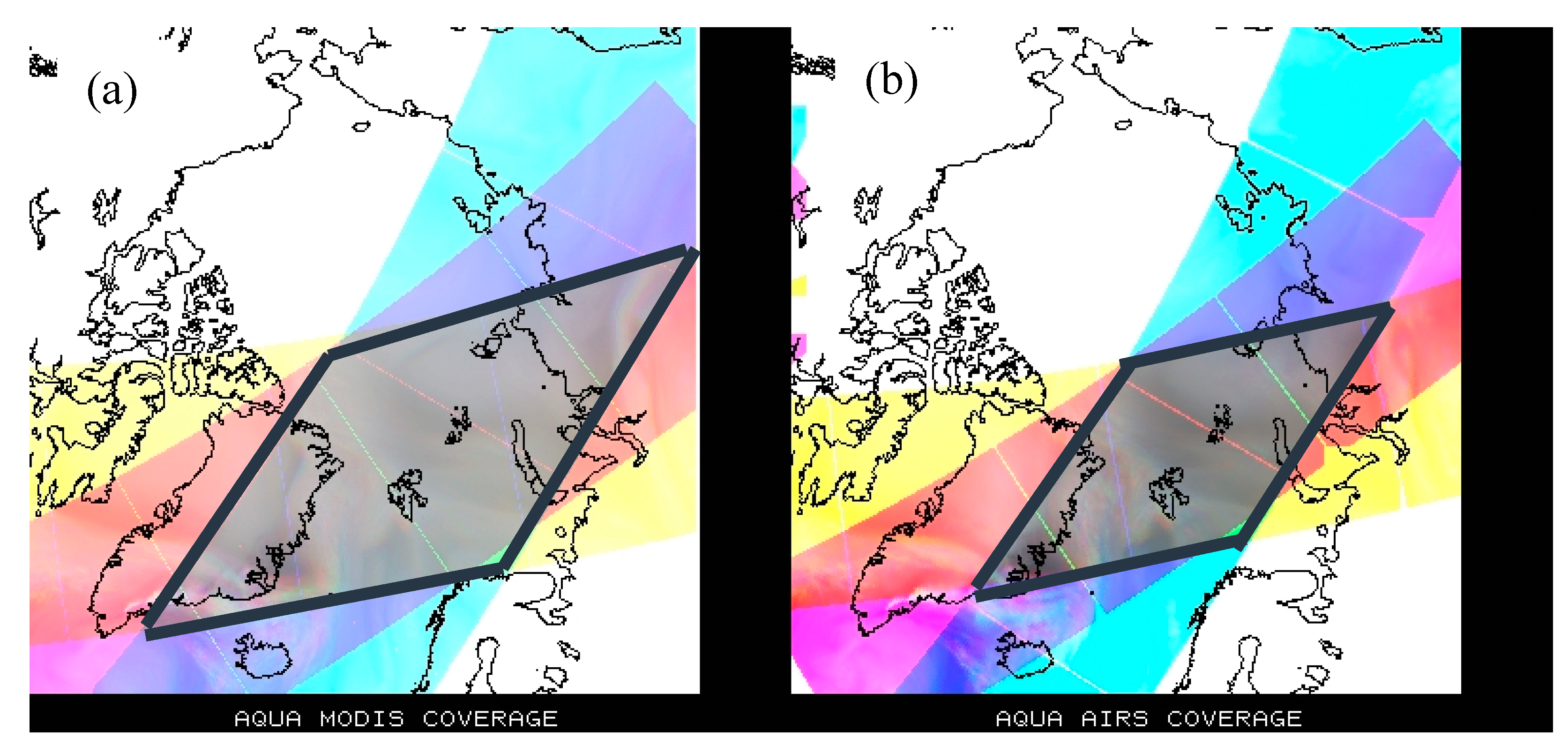
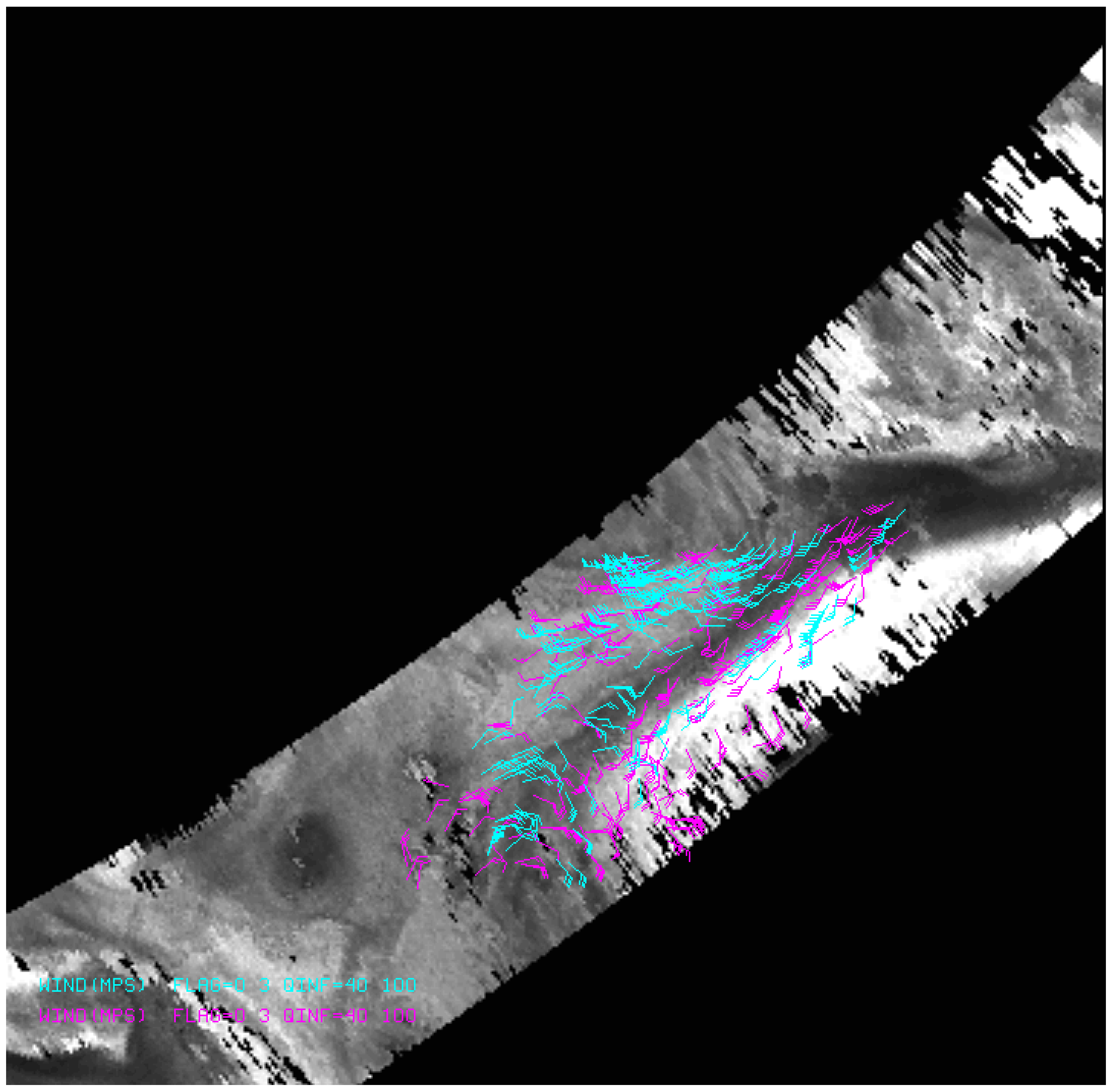
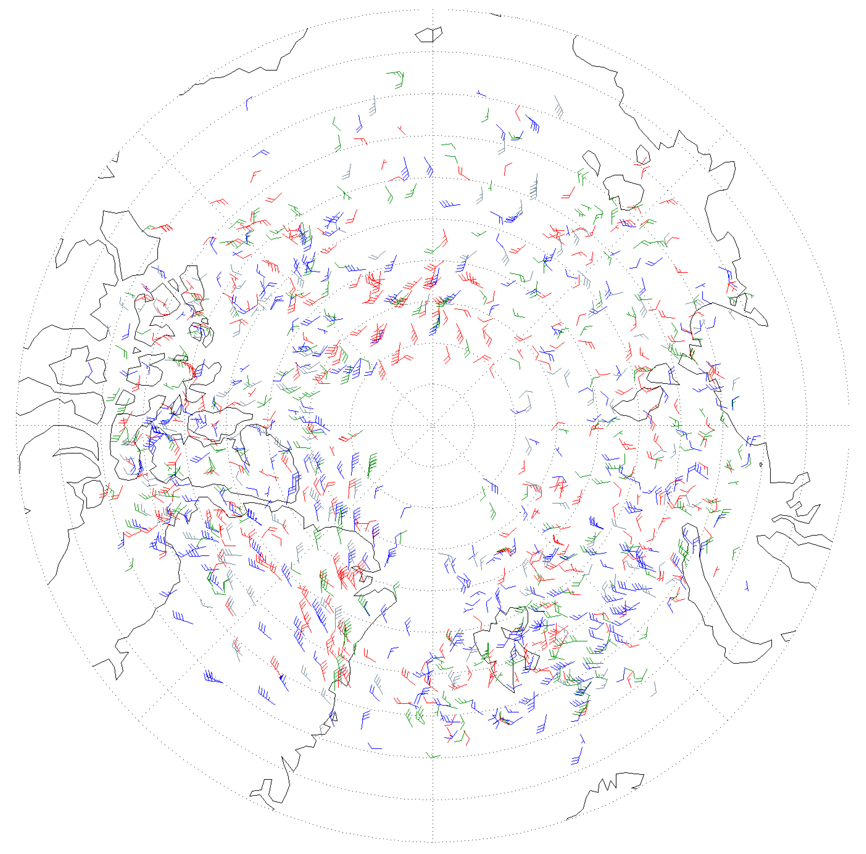
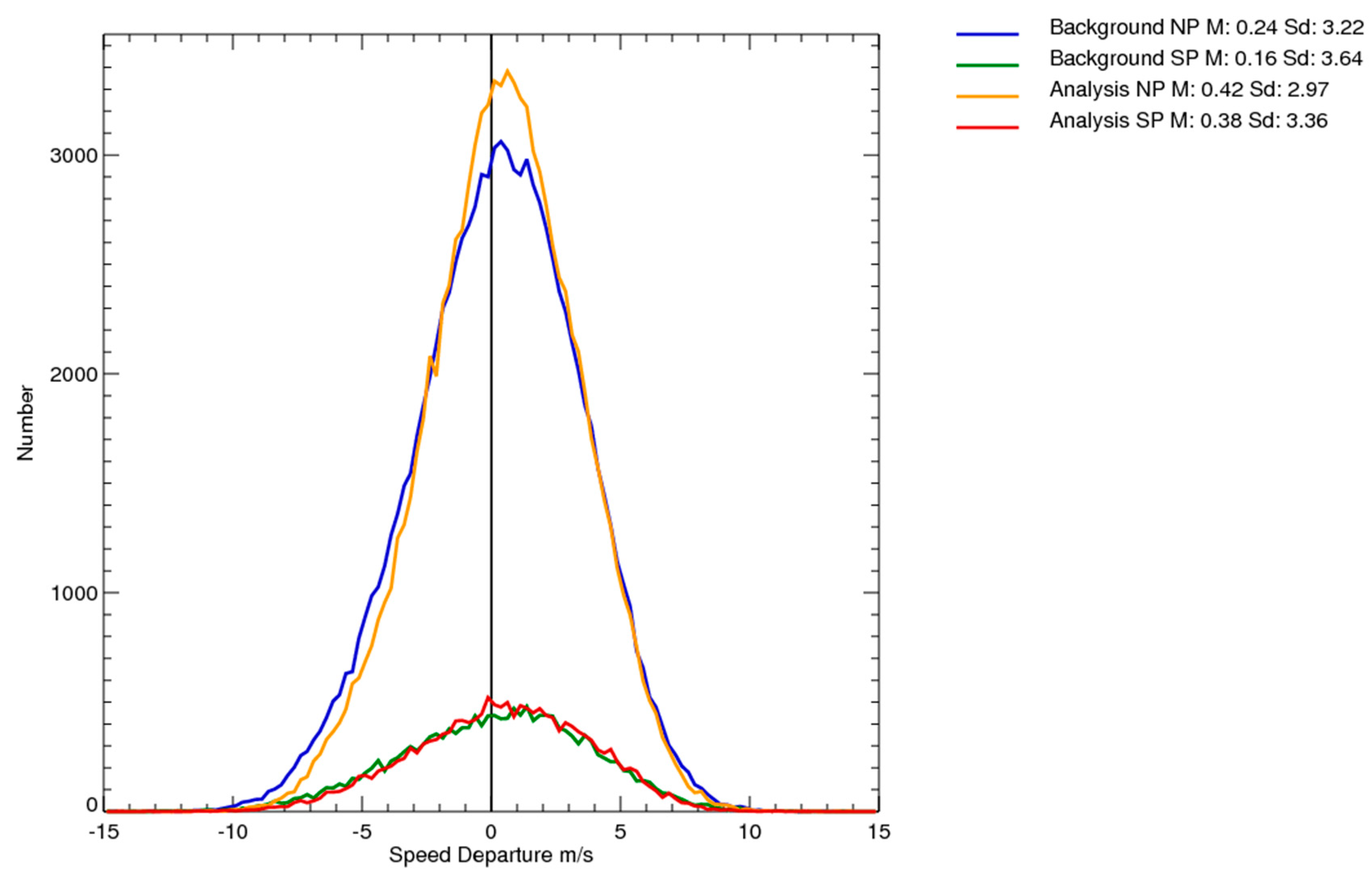
3.1. Comparison of AIRS AMVs to MODIS AMVs

During the northern hemisphere summer, there is more moisture (as compared to winter) resulting in many features to track. For the 14 June to 13 July 2012 time period, 650 wind sets were generated resulting in 164,000 AIRS moisture and 135,000 ozone AMVs. During that same time, nearly 3 million Aqua MODIS winds were generated. The following statistics and results are based on this time period.
AIRS and MODIS AMVs were compared using the following criteria to define co-location: The vectors are located with 25 km of each other and the pressure difference is no more than 15 hPa. This resulted in approximately 24,000 matches or only 8% of the total AIRS winds. This percentage is low for two reasons: the AIRS AMVs are distributed vertically while the MODIS AMVs are at a single level at a specific geographic region and the AIRS dataset contains winds in the stratosphere. In addition, since the AIRS AMVs are only in clear sky and above cloud, the majority of these colocations will be with the MODIS clear sky water vapor AMVs. This is evident in Figure 7, which shows 87% of the matches are from 350 to 425 hPa, which is where the MODIS channel 27 (6.7 µm) peaks in the atmosphere. The very few lower level (higher pressure) winds are likely in very dry regimes where the MODIS channel senses deeper in the atmosphere or where the collocated MODIS AMV is a nearby cloud feature tracked in the IR channel 31 (11 µm).
Figure 8 depicts the distribution of the speed difference between the 24,000 matched AIRS and MODIS AMVs for the northern hemisphere summer. There is no bias (the mean difference is +0.06 ms−1) in this approximately Gaussian distribution. Likewise, the distribution of AMV direction difference (Figure 9) has a near-zero bias. The results are very similar if the histograms (not shown) and statistics are computed separately for the high and low-level AMVs: The mean difference in the high-level winds is 0.00 +/− 3.54 ms−1; the low-level winds mean difference is 0.47 +/− 3.41 ms−1.
These results are encouraging, as the speed and direction differences between the MODIS and AIRS co-located AMVs are similar and with very small bias. Although the standard deviation of the speed difference is several meters per second and direction difference is nearly 14°, this is expected as the low spatial resolution of the AIRS data will result in less precise measuring of the feature motion. In addition, with less than 10% AIRS AMVs being co-located with MODIS winds, the AIRS AMVs should provide unique observations over the high-density MODIS-only dataset.

3.2. Evaluation of AIRS AMVs in the GEOS-5

In addition to comparing AIRS winds to MODIS winds, we ran three NWP experiments to determine the overall impact on numerical forecasts and the relative contributions of each data type (MODIS vs. AIRS). This was done using the GEOS-5 Atmospheric Global Climate Model (AGCM) and was run on the NASA Center for Climate Simulation (NCCS) ‘discover’ system.

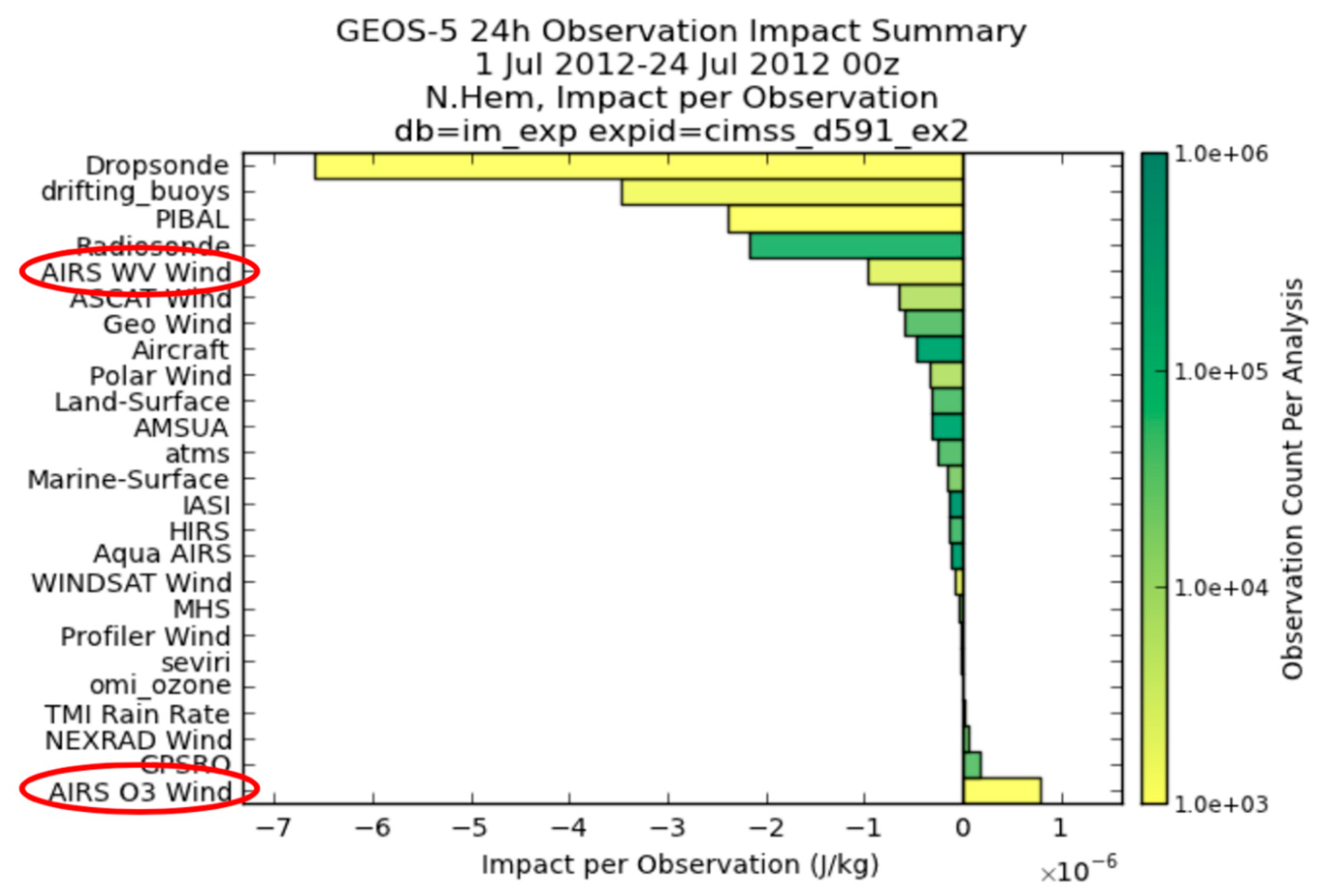
3.2.1. Assimilation Impact

The measure of how well the AIRS AMVs were assimilated in the GEOS-5 was to compare the winds with the GEOS-5 background and analysis fields. Figure 10 depicts the speed departure of the assimilated moisture AMVs from the northern hemisphere background (blue) and northern hemisphere analysis (yellow). However, the results of the northern hemisphere analysis are favorable as the distribution bias of the speed departure is small (approximately 0.2 ms−1). Also, the standard deviation was reduced from 3.2 ms−1 (background) to 3.0 ms−1 (analysis), indicating that the AIRS AMVs that were assimilated had a beneficial impact on the analysis. Since there is very little moisture in the southern hemisphere during winter (green and red curves), they were not considered for this time period.
Figure 11 shows the speed departure for the ozone AMVs that were assimilated. The distributions are skewed (non-Gaussian distributions) and shifted to the right of zero, indicating a fast bias in the AMVs of 1.7 ms−1 for the northern hemisphere, as compared to the background. With very few observations in the stratosphere, it was not possible to determine if the ozone AMVs truly had a fast bias compared to an independent measure of wind speed. However, these AMVs are not parallax adjusted, which if taken into account, would modify the speed by up to several meters per sec and the direction, depending on the viewing angles and altitude of the AMV.
The impact per observation (Figure 12) is very good for the AIRS moisture AMVs, as they are ranked higher than all other satellite-derived wind datasets. This indicates the winds are of good quality. However, the AIRS ozone AMVs have a negative impact, which is likely a result of the large speed bias.

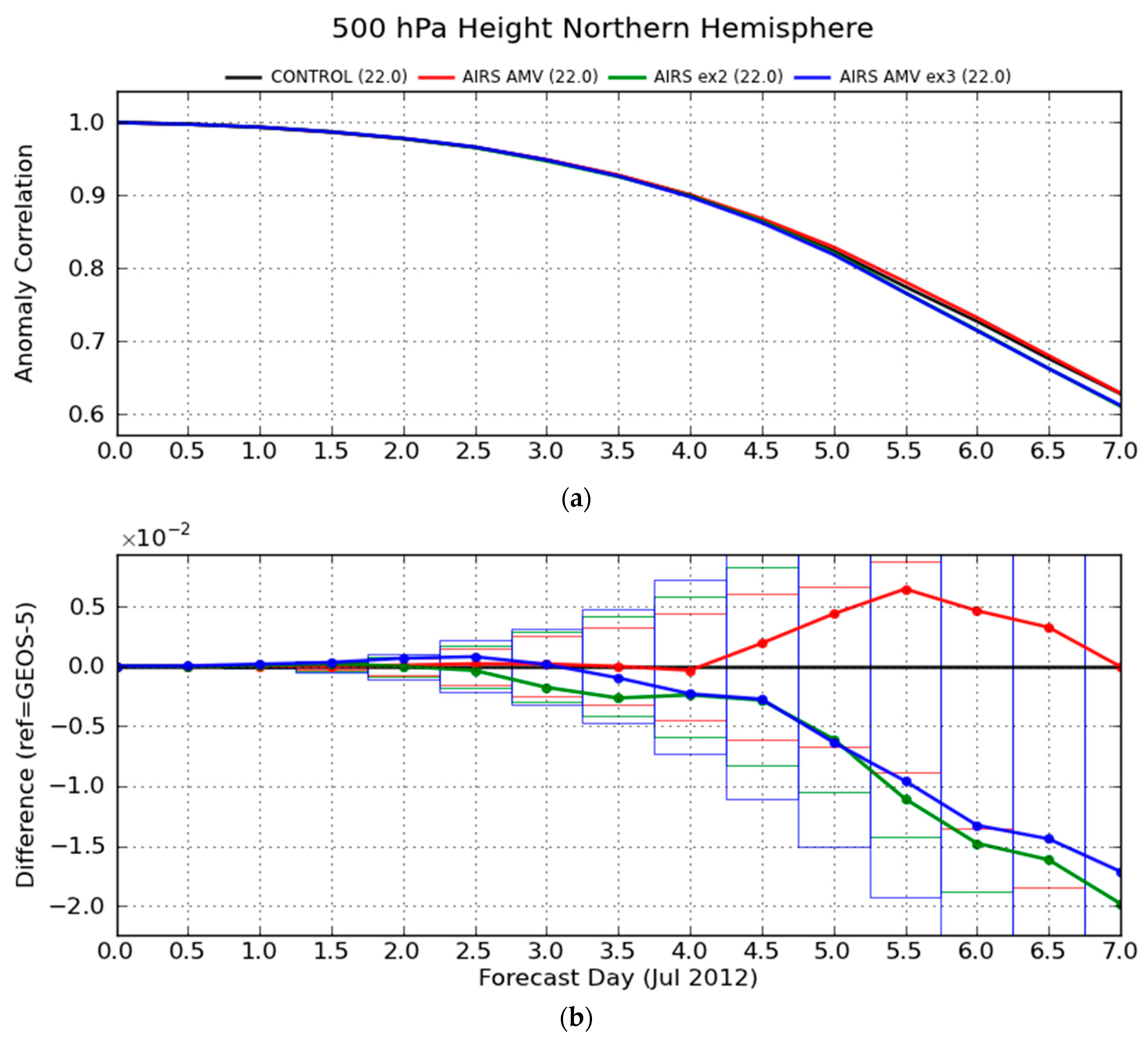
3.2.2. Forecast Impact

The forecast impact was statistically neutral as measured by the Anomaly Correlation Coefficient (ACC) score for the first 24 days of July 2012. Figure 13a depicts the 500 hPa die-off curves for the control (black) and the three experiments:
  • Although not statistically significant, the addition of the AIRS AMVs (red) shows a slight improvement in the ACC score after Day 4 (Figure 13b).
  • The removal of the MODIS AMVs (blue) shows a decrease in the ACC score, as the AIRS AMVs are unable to offset the loss of the MODIS AMVs, indicating that the AIRS AMVs complement the MODIS AMVs and should not be considered a replacement. This was expected as the AIRS AMVs are in clear sky or above cloud regions, while the MODIS AMVs include cloud-tracked features.

3.3. Continuing Evaluation of the AIRS AMVs

The initial positive assessment of the AIRS AMVs described above within this section, has resulted in continued research in this area and the production of the 3D winds routinely at SSEC. In addition, more recent analyses further corroborate the early findings on the usability of this product in NWP applications.
A three-month experiment was run at the NASA Global Modeling and Assimilation Office (GMAO) for the period May through July 2015, which included the AIRS 3D winds [24]. This is an updated GEOS-5 with an assimilation component that is a three-dimension variational/ensemble hybrid (3D-Hybrid) scheme that is run at 0.5°, with the ensembles running at 1.0° resolution. The model at this time ran at 1/4° horizontal resolution globally and at 72 vertical levels up to 0.01 hPa.
Additional comparisons with the MODIS winds show improved vertical coverage and equivalent observation departures, which are depicted in the following figures. Figure 14 shows the normalized observation count per 6-h cycle for the AIRS retrieval AMVs (red) and MODIS water vapor AMVs (black) for the northern hemisphere. Of importance is that the AIRS retrieval-derived AMVs result in a higher percentage of wind observations in the mid-troposphere (below 500 hPa) than MODIS. This analysis quantifies the improvement in the vertical extent of the 3D winds product, which was qualitatively evident in Figure 6.
The mean and standard deviation of the observation departures, or the difference between the observation and the 6-h forecast, is shown in Figure 15 for the AIRS and MODIS water vapor winds. Minimal quality control is applied to eliminate large outliers. It is seen that the MODIS winds have a persistent negative bias above 300 hPa, but the AIRS winds do not have any measurements at these levels. Similar biases in magnitude are seen 500 and 300 hPa for both instruments, though not necessarily of a similar sign. From 500 to 600 hPa, MODIS shows an increase in the bias not reflected in the AIRS observations. It is also noted though, that the observation counts below 500 hPa are very small for MODIS. For AIRS, the bias is largest in magnitude below 700 hPa, though this is again a layer of few observations. When considering the standard deviations, the MODIS observations show less variance than AIRS at layers above 500 hPa, and AIRS shows less variance at regions below 500 hPa. Both show a reduction in variance to about 500 hPa, while the variance is more consistent layer-to-layer below that point.
In addition to the NASA GMAO, the Fleet Numerical Meteorology and Oceanography Center (FNMOC) also assimilated AIRS AMVs into their Navy Atmospheric Variational Data Assimilation System—Accelerated Representer (NAVDAS-AR). This is a 4D-Var system with advanced variational bias correction. A 3-week period beginning in late June 2015 was evaluated and they came to a similar conclusion [25]:
…the ob impact stats looked OK and they are comparable to other polar winds in impact per ob. The innovation statistics were also similar to other polar winds. The problem is that there just aren’t enough of them to make much of an impact.

4. Discussion

This end-to-end study (from product generation to NWP forecast impact) provides a baseline capability to derive wind information from tracking moisture features derived from hyperspectral IR instruments, in clear sky and above cloud. Even though the spatial resolution of the AIRS instrument (13.5 km) is much reduced compared to the resolution typical of imagers on the current weather satellites (2–4 km), useful AMVs were derived.
Since these AMVs are derived only in the polar regions, validating the product is difficult because AMVs are traditionally compared to rawinsondes, which are very sparse at high latitudes. In this case, we compared with both MODIS AMVs (which are derived from the MODIS instrument on Aqua) and evaluated the data assimilation and forecast impacts. Because the MODIS winds are derived at a single pressure level at a given location, the number of co-locations was small (less than 10% of the total number of AIRS AMVs) over a one-month period. The result was a speed difference of approximately zero meters per second between the MODIS and AIRS winds. That, along with a standard deviation of 3.5 ms−1, provides reasonable assurance that the AIRS AMVs have a similar quality to the MODIS AMVs. This is further substantiated in the Impact per Observation from the GEOS-5, which rated the AIRS moisture winds just below the impact due to radiosondes. This was not the case for the AIRS ozone winds in the stratosphere, which we suspect is partly due to not accounting for parallax in computing the AMVs and the impact metric is based on tropospheric changes. This fast bias was observed in the comparison with the model background.
The assimilation statistics have been consistent beginning with the first experiments in 2013 with a 3DVar GEOS-5, to the 3D Hybrid ensemble GEOS-5 in 2015, and the evaluation at FNMOC using the NAVDAS-AR 4DVar system in 2015. Although the forecast impact was not statistically significant, it was positive, especially in days 4.5 to 6.5 in the one-month experiment. This is very encouraging because the vertical and spatial density of winds is low for the current product and the winds are only in the high latitudes, but they have positive impact in the northern hemisphere correlation scores. This is similar to the impact of the MODIS polar winds, as it takes several days for the information to propagate from the polar regions to have a hemispheric impact on the forecast, as measured by the ACC score. Moreover, these improvements are most significant on specific days of a case study, in situations where high-latitude systems were better captured with the polar winds, that eventually affect mid-latitude dynamics [26]. Since the AIRS AVMs have a similar quality as the MODIS winds (as measured by the observation departures in the GEOS-5), a statistically significant forecast impact is expected by the 3D winds product, once it is extended to deriving AMVs from the additional sounders (CrIS and IASI) on polar orbiting platforms.

5. Conclusions

From this study of deriving atmospheric motion from retrieved moisture fields as sensed by the AIRS instrument, we found:
  • The AIRS AMVs compare favorably to co-located MODIS AMVs for a six-week period, as evidenced by a zero-speed bias with a standard deviation of 3.5 ms−1.
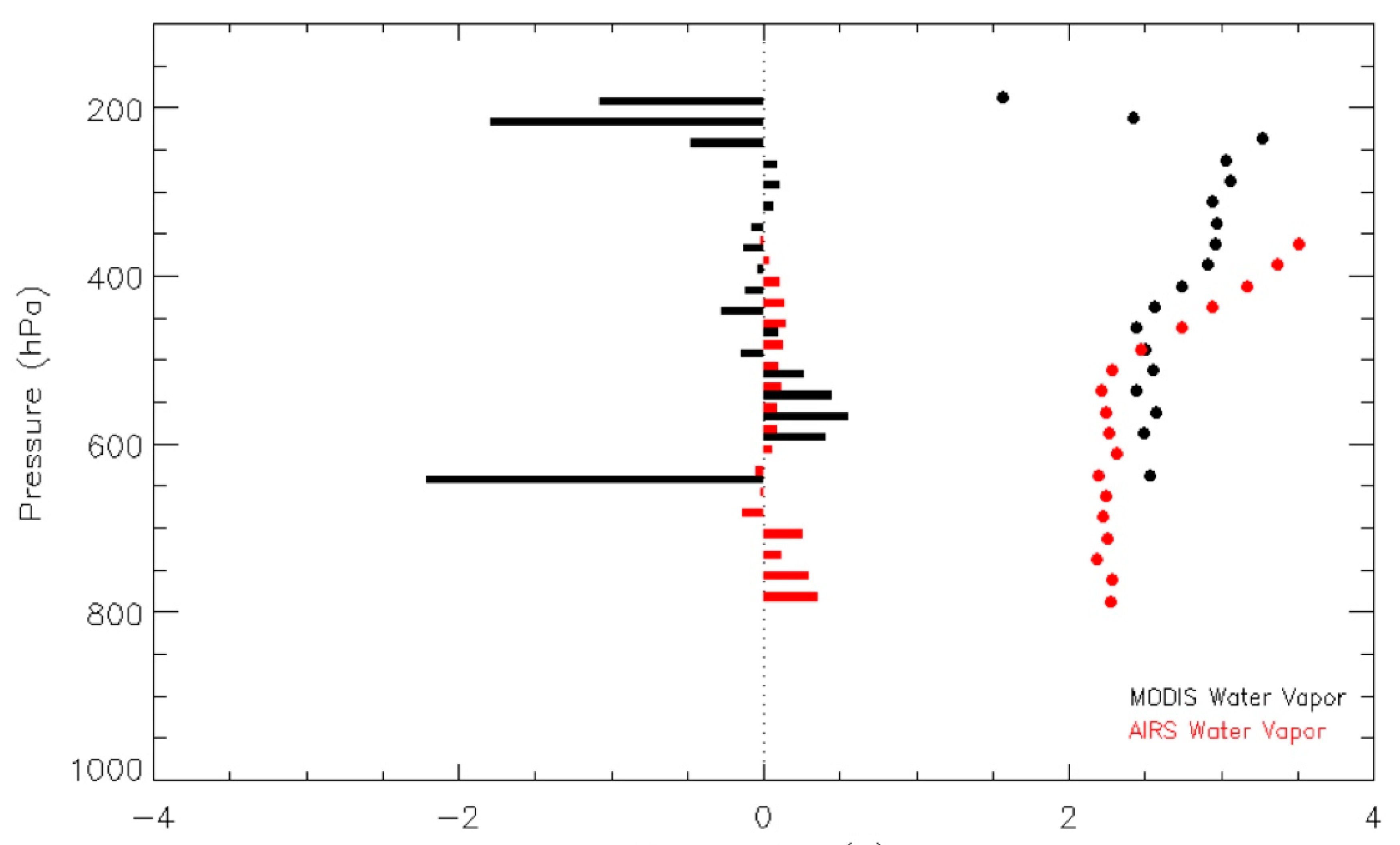
  • The impact per AIRS moisture AMV is very good, as they are ranked higher than all other satellite-derived wind datasets.
  • The neutral, or slightly positive, forecast impact due to the addition of the AIRS retrieval AMVs is encouraging as these AMVs are only in the polar region, but they have an impact in the longer-range forecast over the northern hemisphere.
The AIRS AMV product continues to be produced routinely at SSEC as part of NASA grant 80NSSC18K0984. This current project will expand the generation of AMVs to the CrIS and IASI instruments, evaluate optical flow for deriving the winds, determine better error estimates (in collaboration with the Jet Propulsion Lab), and run additional NWP experiments (to be conducted by the NASA GMAO). The current assimilation component at the GMAO is the Atmospheric Data Assimilation System (ADAS), which is ensemble-based in three and four dimensions [27].
The above effort will improve the spatial coverage of the current 3D winds product, but a more significant NWP impact could be realized with a higher resolution sounder to retrieve more accurate AMVs. This could be done with a constellation of small polar-orbiting satellites flying in formation (in a similar orbit but time separated) to track moisture features over time (Figure 16), or by placing a hyperspectral sounder on a geostationary satellite, which has been done recently by China with their Geostationary Interferometric Infrared Sounder (GIIRS) on FY4A and will be part of EUMETSAT’s Meteosat Third Generation (MTG) satellites in the early 2020s.

Author Contributions

Conceptualization, D.S. (David Santek); Data curation, D.S. (Dave Stettner); Funding acquisition, D.S. (David Santek); Investigation, D.S. (David Santek); Methodology, D.S. (David Santek) and S.N.; Software, S.N. and D.S. (Dave Stettner); Supervision, D.S. (David Santek); Validation, D.S. (David Santek) and S.N.; Visualization, S.N. and D.S. (Dave Stettner).

Funding

This research was funded by NASA, grants NNX11AE97G, NNX14AI77G, and 80NSSC18K0984. The APC was funded by NASA grant 80NSSC18K0984.

Acknowledgments

Dagmar Merkova configured and facilitated the running of the GEOS-5 at the NASA GMAO. Will McCarty of the NASA GMAO provided several figures on his independent analysis of the 3D AMVs as compared to the GEOS-5 model background.

Conflicts of Interest

The authors declare no conflict of interest. Also, the funders had no role in the design of the study; in the collection, analyses, or interpretation of data; in the writing of the manuscript, or in the decision to publish the results.

References

  1. Breitman, K. Failure to Prepare for Extreme Weather Costs Billions. USA Today. 2014. Available online: http://www.usatoday.com/story/news/nation/2014/02/12/costs-unpreparedness-critical-weatherevents/5417257/ (accessed on 1 July 2019).
  2. Gentry, B.; Atlas, R.; Baker, W.; Emmitt, G.D.; Hardesty, R.M.; Kakar, R.; Kavaya, M.; Mango, S.; Miller, K.; Riishojgaard, L.P. Recent US Activities Toward Development of a Global Tropospheric 3D Wind Profiling System. In Proceedings of the American Geophysical Union Fall Meeting, San Francisco, CA, USA, 15–19 December 2008. [Google Scholar]
  3. Dessler, A.E.; Palm, S.P.; Spinhirne, J.D. Tropical cloud-top height distributions revealed by the Ice, Cloud, and Land Elevation Satellite (ICESat)/Geoscience Laser Altimeter System (GLAS). J. Geophys. Res. 2006, 111, D12215. [Google Scholar] [CrossRef]
  4. A Community Assessment and Strategy for the Future, Earth Science and Applications from Space. National Imperatives for the Next Decade and Beyond; National Research Council: Washington, DC, USA, 2007; ISBN 0-309-66714-3.
  5. Zeng, X.; Ackerman, S.; Ferraro, R.D.; Murray, J.J.; Pawson, S.; Reynolds, C.; Teixeira, J. Workshop Report on Scientific Challenges and Opportunities in the NASA Weather Focus Area; NASA: Washington, DC, USA, 2015.
  6. Keyser, D. On the representation and diagnosis of frontal circulations in two and three dimensions. In The Life Cycles of Extratropical Cyclones; Shapiro, M.A., Gronas, S., Eds.; American Meteorological Society: Boston, MA, USA, 1999; pp. 239–264. [Google Scholar]
  7. Pu, B.; Cook, K.H. Dynamics of the West African Westerly Jet. J. Clim. 2010, 23, 6263–6276. [Google Scholar] [CrossRef]
  8. Baker, W.E.; Atlas, R.; Cardinali, C.; Clement, A.; Emmitt, G.D.; Gentry, B.M.; Hardesty, R.M.; Källén, E.; Kavaya, M.J.; Langland, R.; et al. Lidar-Measured Wind Profiles: The Missing Link in the Global Observing System. Bull. Am. Meteorol. Soc. 2014, 95, 543–564. [Google Scholar] [CrossRef]
  9. Charron, M.; Polavarapu, S.; Buehner, M.; Vaillancourt, P.A.; Charette, C.; Roch, M.; Morneau, J.; Garand, L.; Aparicio, J.M.; MacPherson, S.; et al. The Stratospheric extension of the Canadian global deterministic medium-range weather forecasting system and its impact on tropospheric forecasts. Mon. Weather. Rev. 2012, 140, 1924–1944. [Google Scholar] [CrossRef]
  10. Kidston, J.; Scaife, A.; Hardiman, S.; Mitchell, D.; Butchart, N.; Baldwin, M.; Gray, L. Stratospheric influence on tropospheric jet streams, storm tracks and surface weather. Nat. Geosci. 2015, 8, 433–440. [Google Scholar] [CrossRef]
  11. Menzel, W.P. Cloud tracking with satellite imagery: From the pioneering work of Ted Fujita to the present. Bull. Am. Meteorol. Soc. 2001, 82, 33–47. [Google Scholar] [CrossRef]
  12. Key, J.R.; Santek, D.; Velden, C.S.; Bormann, N.; Thépaut, J.-N.; Riishojgaard, L.P.; Zhu, Y.; Menzel, W.P. Cloud-Drift and Water Vapor Winds in the Polar Regions from MODIS. IEEE Trans. Geosci. Remote Sens. 2003, 41, 482–492. [Google Scholar] [CrossRef]
  13. Santek, D. The Global Impact of Satellite-Derived Polar Winds on Model Forecasts. Ph.D. Thesis, University of Wisconsin-Madison, Madison, WI, USA, 2007. [Google Scholar]
  14. Susskind, J.; Barnet, C.D.; Blaisdell, J.M. Retrieval of atmospheric and surface parameters from AIRS/AMSU/HSB data in the presence of clouds. IEEE Trans. Geosci. Remote Sens. 2003, 42, 390–409. [Google Scholar] [CrossRef]
  15. Goldberg, M.D.; Qu, Y.; McMillin, L.M.; Wolf, W.; Zhou, L.; Divakarla, M. AIRS near-real-time products and algorithms in support of operational numerical weather prediction. IEEE Trans. Geosci. Remote Sens. 2003, 41, 379–389. [Google Scholar] [CrossRef]
  16. Weisz, E.; Li, J.; Menzel, W.P.; Heidinger, A.K.; Kahn, B.H.; Liu, C.-Y. Comparison of AIRS, MODIS CloudSat and CALIPSO cloud top height retrievals. Geophys. Res. Lett. 2007, 34, L17811. [Google Scholar] [CrossRef]
  17. Weisz, E.; Smith, W.L.; Li, J.; Menzel, W.P.; Smith, N. Improved Profile and Cloud Top Height Retrieval by Using Dual-regression on High-Spectral Resolution Measurements. In Proceedings of the Hyperspectral Imaging and Sounding of the Environment (HISE), Toronto, ON, Canada, 10–14 July 2011; OSA Technical Digest Series (CD) Optical Society of America: Washington, DC, USA, 2011. [Google Scholar]
  18. Weisz, E.; Smith, W.L.; Smith, N. Advances in simultaneous atmospheric profile and cloud parameter regression-based retrieval from high-spectral resolution radiance measurements. J. Geophys. Res. Atmos. 2013, 118, 6433–6443. [Google Scholar] [CrossRef]
  19. Smith, W.L.; Weisz, E.; Kirev, S.; Zhou, D.K.; Li, Z.; Borbas, E.E. Dual-Regression Retrieval Algorithm for Real-Time Processing of Satellite Ultraspectral Radiances. J. Appl. Meteorol. Clim. 2012, 51, 1455–1476. [Google Scholar] [CrossRef]
  20. Hautecoeur, O.; Héas, P.; Borde, R. Extraction of 3D wind profiles from IASI level 2 products. In Proceedings of the Thirteenth International Winds Workshop, Monterey, CA, USA, 27 June–1 July 2016. [Google Scholar]
  21. Holmlund, K. The utilization of statistical properties of satellite−derived atmospheric motion vectors to derive quality indicators. Weather Forecast. 1998, 12, 1093–1103. [Google Scholar] [CrossRef]
  22. Hayden, C.; Pursor, R.J. Recursive filter objective analysis of meteorological fields: Applications to NESDIS operational processing. J. Appl. Meteorol. 1995, 34, 3–15. [Google Scholar] [CrossRef]
  23. Rienecker, M.M.; Suarez, M.J.; Todling, R.; Bacmeister, J.; Takacs, L.; Liu, H.-C.; Gu, W.; Sienkiewicz, M.; Koster, R.D.; Gelaro, R.; et al. The GEOS-5 Data Assimilation System—Documentation of Versions 5.0.1, 5.1.0, and 5.2.0; Technical Report Series on Global Modeling and Data Assimilation; NASA/GSFC: Greenbelt, MD, USA, 2008; p. 27.
  24. McCarty, Will (NASA/GMAO), 2015, e-mail message to author, October 15.
  25. Pauley, Randy (FNMOC), 2015, e-mail message to author, September 15.
  26. Santek, D. The Impact of Satellite-Derived Polar Winds on Lower-Latitude Forecasts. Mon. Weather Rev. 2010, 138, 123–139. [Google Scholar] [CrossRef]
  27. GEOS Systems. Available online: https://gmao.gsfc.nasa.gov/GEOS/ (accessed on 29 October 2019).
Figure 1. A vertical cross-section of the atmospheric motion vectors for a six-hour period centered on 00 UTC on 10 December 2014 between 5°S and 5°N.
Remotesensing 11 02597 g001
Figure 2. An example of temperature and dewpoint profiles for clear sky (a), above low cloud (b), above high cloud (c) as compared to the model background. Retrievals (black) and NCEP/GFS (magenta).
Remotesensing 11 02597 g002
Figure 3. Three successive overlapping passes (each separated by 100 min) of radiance images from the (a) Aqua Moderate Resolution Imaging Spectroradiometer (MODIS) and the (b) Atmospheric Infrared Sounder (AIRS). The region of intersection (gray parallelograms) shows where features can be tracked.
Remotesensing 11 02597 g003
Figure 4. AIRS retrieval atmospheric motion vectors (AMVs) over a 400 hPa AIRS retrieved moisture field from 20 July 2012 0551 UTC. The North Pole is in the center of the picture, with Greenland in the lower-left region (not visible). These wind barbs are all moisture and ozone tracked AMVs color- coded by pressure level: cyan 400 to 699 hPa; magenta above 399 hPa.
Remotesensing 11 02597 g004
Figure 5. All derived winds from 5 January 2011 color-coded by level: 700–600 hPa (red), 550–450 hPa (green), 400–300 hPa (blue), 150 hPa ozone (gray).
Remotesensing 11 02597 g005
Figure 6. Vertical distribution of AIRS retrieval winds over the north pole region: (a) upper panel is ozone AMVs; (b) lower panel is humidity AMVs. All derived winds from 6 January 2011 at 1200 UTC. Colors denote distance from the north pole: blue (far) to red (close). Gray is a model analysis. Note: This is one-half day of winds, which results in one-half of the daily longitudinal coverage.
Remotesensing 11 02597 g006
Figure 7. Histogram of the pressures for co-located Aqua MODIS and AIRS retrieval AMVs for a northern hemisphere summer case: 14 June to 31 July 2012. Since both the AIRS and MODIS AMVs are on discrete (but different) pressure levels, the resulting histogram is depicted of discontinuous frequency bars, at the AIRS AMV pressure levels, which are approximately every 16 hPa from 359 to 424 hPa. The MODIS AMVs are assigned pressures to the nearest 12.5 hPa.
Remotesensing 11 02597 g007
Figure 8. Histogram of the speed difference between co-located Aqua MODIS and AIRS retrieval AMVs for a northern hemisphere summer case: 14 June to 31 July 2012. Mean = +0.06 ms−1; Standard Deviation = 3.53 ms−1.
Remotesensing 11 02597 g008
Figure 9. Histogram of the direction difference between co-located Aqua MODIS and AIRS retrieval AMVs for a northern hemisphere summer case: 14 June to 31 July 2012. Mean = −0.08°; Standard Deviation = 13.90°.
Remotesensing 11 02597 g009
Figure 10. Distribution of speed departure for 01–29 July 2012 for the AIRS moisture AMVs. Compared to the background (Arctic—blue; Antarctic—green) and analysis (Arctic—yellow; Antarctic—red).
Remotesensing 11 02597 g010
Figure 11. Distribution of speed departure for 01–29 July 2012 for the AIRS ozone AMVs. Compared to the background (Arctic—blue; Antarctic—green) and analysis (Arctic—yellow; Antarctic—red).
Remotesensing 11 02597 g011
Figure 12. Impact per observation for 01–24 July 2012 0000 UTC for the AIRS WV (moisture) and O3 (ozone) AMVs.
Remotesensing 11 02597 g012
Figure 13. The 500 hPa Northern Hemisphere ACC die-off curves (a) for 1–24 July 2012 00 UTC. The control (black) and three experiments (red, green, and blue) are shown. The lower figure (b) shows the difference between the control and the experiments. A positive difference is an improvement in the forecast; to be statistically significant, the curve must lie outside of its threshold rectangle.
Remotesensing 11 02597 g013
Figure 14. Vertical histogram showing the normalized observation counts per 6-h assimilation cycle for MODIS (black) and AIRS (red) water vapor AMVs. These are for all AMVs in the GEOS assimilation system before thinning or quality control, every six hours from 0000 UTC 1 May 2015 to 1800 UTC 31 Jul 2015.
Remotesensing 11 02597 g014
Figure 15. Mean (bars) and standard deviation (circles) of observation departures (m s−1) (observed minus 6-h forecasted wind) for MODIS (black) and AIRS (red) water vapor AMVs 0000 UTC 1 May 2015 to 1800 UTC 31 July 2015.
Remotesensing 11 02597 g015
Figure 16. An artist’s conception of two time-separated satellites equipped with hyperspectral IR sounders that can provide moisture data cubes in the troposphere, resulting in winds at multiple pressure levels (lower right).
Remotesensing 11 02597 g016

