Deriving Field Scale Soil Moisture from Satellite Observations and Ground Measurements in a Hilly Agricultural Region


1
Department of Geodesy and Geoinformation, TU Wien, 1040 Vienna, Austria
2
Institute of Photogrammetry and Remote Sensing, Technische Universität Dresden, 01069 Dresden, Germany
*
Author to whom correspondence should be addressed.
Remote Sens. 2019, 11(22), 2596; https://doi.org/10.3390/rs11222596
Submission received: 3 September 2019
/
Revised: 31 October 2019
/
Accepted: 4 November 2019
/
Published: 6 November 2019
(This article belongs to the Special Issue Remote Sensing of Regional Soil Moisture)
Abstract
:Agricultural and hydrological applications could greatly benefit from soil moisture (SM) information at sub-field resolution and (sub-) daily revisit time. However, current operational satellite missions provide soil moisture information at either lower spatial or temporal resolution. Here, we downscale coarse resolution (25–36 km) satellite SM products with quasi-daily resolution to the field scale (30 m) using the random forest (RF) machine learning algorithm. RF models are trained with remotely sensed SM and ancillary variables on soil texture, topography, and vegetation cover against SM measured in the field. The approach is developed and tested in an agricultural catchment equipped with a high-density network of low-cost SM sensors. Our results show a strong consistency between the downscaled and observed SM spatio-temporal patterns. We found that topography has higher predictive power for downscaling than soil texture, due to the hilly landscape of the study area. Furthermore, including a proxy of vegetation cover results in considerable improvements of the performance. Increasing the training set size leads to significant gain in the model skill and expanding the training set is likely to further enhance the accuracy. When only limited in-situ measurements are available as training data, increasing the number of sensor locations should be favored over expanding the duration of the measurements for improved downscaling performance. In this regard, we show the potential of low-cost sensors as a practical and cost-effective solution for gathering the necessary observations. Overall, our findings highlight the suitability of using ground measurements in conjunction with machine learning to derive high spatially resolved SM maps from coarse-scale satellite products.

1. Introduction
By modulating the water, carbon, and energy fluxes between the soil, the vegetation, and the atmosphere, soil moisture is a key variable in climatological and hydrological processes and a regulator of productivity in agricultural systems. It affects the partitioning of water between infiltration, runoff, and evapotranspiration, thus governing the water available for photosynthesis. Accurate knowledge of the spatial and temporal patterns of moisture conditions is required for crop yield estimation [1,2], drought monitoring [3,4,5,6], weather and climatic prediction [7,8,9], rainfall-runoff response [10,11,12], and landslide forecasting [13,14].
Different factors govern and affect soil moisture patterns across scales: Point- and field-scale variations in space are mainly caused by topography, soil texture, and vegetation, while regional- and continental-scale patterns are controlled by meteorological forcing [15,16]. Hence, monitoring soil moisture is challenging because of its high variability both in space and in time. In-situ sensors provide accurate and reliable measurements at the point scale, however they are costly, and their installation and maintenance are time consuming. Therefore, in-situ sensors are limited in number on a global basis [17,18,19]. Due to their sparsity, available ground stations can only provide an incomplete picture of the moisture conditions over large areas, making their use impractical for large-scale monitoring [20]. On the other hand, remotely sensed data from microwave sensors have been successfully used to retrieve soil moisture globally [21,22]. This is possible because of the high contrast between dielectric properties of liquid water and dry soil, which can be related either to the microwave emission or to the backscatter detected by passive and active microwave sensors, respectively. However, a trade-off between the spatial and temporal resolution of remotely sensed soil moisture products exists. Synthetic aperture radar (SAR) systems can retrieve data at (sub-) field scale but are characterized by a long revisit time. For example, the recently launched Sentinel-1 mission is used to retrieve surface soil moisture at 1 km with a revisit time of up to four days over Europe [23]. Consequently, short-term events such as rainfall often cannot be captured. Passive (radiometers) and active (radars) microwave sensors with large footprints can observe the same location daily or sub-daily, but typically have spatial resolutions in the order of tens of km. Therefore, such coarse-scale products can capture the temporal dynamics of soil moisture but are inadequate in providing spatial details.
Several agricultural and hydrological applications would benefit from soil moisture observations with a sub-kilometer spatial resolution while preserving a daily revisit time [24,25]. To meet these requirements, several downscaling approaches have been developed, differing in terms of input data and scaling models. Generally, the attainable resolution of the soil moisture downscaled using auxiliary data (e.g., land surface attributes, optical and/or radar remote sensing) depends on the resolution of these auxiliary data. The downscaling method used to describe the relationship between the coarse-scale soil moisture and the local variability can be either statistical or physically based. A comprehensive review of downscaling methods for remotely sensed soil moisture products, discussing assumptions, advantages, and disadvantages associated with each method, is given in Peng et al. [26] and Sabaghy et al. [27].
Over the last decade, machine learning methods have been introduced to downscale soil moisture products and were found to be superior to other techniques [27]. A common way to use machine learning algorithms is to build a model between the coarse-scale soil moisture as the response variable and ancillary surface parameters aggregated to the same coarse resolution as explanatory variables. The model is then applied to the native resolution of those explanatory variables [28], thus assuming that the relationship between soil moisture and ancillary variables remains constant among scales. However, uncertainties and errors arise when aggregating high-resolution surface variables to coarse scale, because of smoothing effects [29]. Zhao et al. [30] clearly presented this issue by taking the elevation as an example: At 1 km resolution, it varied between 4 m and 2418 m, while after the spatial aggregation to 36 km, elevation ranged between 152 m and 1507 m. Extreme values are smoothed after spatial averaging, thus are not included in the training data. To avoid such shortcoming, one could derive robust relationships between coarse-scale soil moisture products and high-resolution ancillary variables using in-situ measurements. However, extensive in-situ observations would be a prerequisite for training the model. Moreover, the accuracy of model predictions increases with increasing the number of samples used as the training set [31]. The limited number of in-situ observations available has been a limiting factor for the application of such a downscaling approach [26].
An appealing solution is offered by low-cost soil moisture sensors, which have gained great attention in the last decade. A large variety of sensors with different measuring techniques and objectives has been developed recently [32,33,34]. In particular, capacitance sensors found widespread use because they are relatively inexpensive and easy to operate. The significantly lower cost of these sensors compared to traditional probes makes them suitable for high-density and/or large-scale monitoring of soil moisture [35,36]. Increasing the number of sensors in a network further reduces the sampling error due to the high spatial variability of soil moisture [37].
Here, we aim to downscale coarse resolution (25–236 km) satellite soil moisture products to high spatial (30 m) resolution, in order to meet the requirements of agricultural and hydrological applications. The downscaling framework is based on the random forest machine learning algorithm trained against in-situ soil moisture measurements. Coarse-scale soil moisture products and ancillary information on soil texture, topography, and temporal dynamics of vegetation are used as model predictors. A high-density network of low-cost sensors was installed in an agriculturally dominated catchment in Austria to develop and test the proposed downscaling approach. The main objectives of this study were to (i) assess the robustness of the downscaling model, in relation to environmental conditions and physical properties of the study area, (ii) evaluate the impact of different input variables on the model accuracy, and finally, (iii) estimate the effect of various training sets, differing in terms of size and sampling schemes (spatially limited and temporally limited scenarios), on the model skill.
2. Materials and Methods
2.1. Study Area
The hydrological open air laboratory (HOAL, [38]) is an agricultural catchment (66 ha) located in Petzenkirchen, lower Austria (48°9′N, 15°9′E) (Figure 1a). The area is characterized by a humid climate with higher precipitation in summer than in winter. The mean annual temperature and precipitation measured during the period 1990–2014 are 9.5 °C and 823 mm year−1, respectively. The mean annual evapotranspiration estimated for the same period is 628 mm year−1 [38]. The elevation ranges from 268 to 323 m a.s.l. with a mean slope of 8%. The dominant soil types in the catchment are Cambrisols and Planosols, characterized by medium to poor infiltration capacities [38].
Most of the catchment area is arable land (87%), while the rest is forested (6%), used as pasture (5%), or paved (2%). Usually, winter crops (mainly wheat) are planted in November and harvested in June, while summer crops (mainly maize) are planted in April and harvested in October. Depending on the crop and the weather conditions, these dates might vary by a few weeks.
2.2. In-Situ Measurements
Since April 2017, an in-situ network of low-cost sensors (Flower Power, Parrot [39]) measuring both soil moisture and incoming solar radiation has been installed in the catchment [36]. The selection of the sensor locations follows the design employed by Vreugdenhil et al. [40] for the validation of coarse-scale soil moisture products over the same area [41]. In this study, we used 38 low-cost sensors covering a wide range of soil texture and topographic conditions (Supplementary Figures S1 and S2). Nineteen sensors were installed within agricultural fields and temporarily removed during field management practices (planting, harvesting, ploughing, etc.) and are referred to as CROP (Supplementary Figure S3). The remaining 19 sensors were permanently positioned in forest and grassland sites, as well as at the edges of agricultural fields (NO-CROP, Figure 1b). The original readings of the low-cost sensors, taken every 15 min, were resampled to daily averages.
2.2.1. Soil Moisture
A capacitance sensor inserted vertically in the top layer of the soil (approximately 7 cm) measures the soil capacitance, which is related to the dielectric permittivity. The latter is then converted to volumetric soil moisture using a predefined calibration equation [36]. An extensive evaluation of the low-cost sensor performances was carried out both in the laboratory and in the field, proving the capability of this sensor to reliably observe soil moisture [36]. Measurements from the low-cost sensors have been evaluated against gravimetric observations in the lab for the dominant soil type present in the catchment [36]. Several water content levels have been investigated, ranging from air dry to full saturation. For each soil moisture level considered, five low-cost sensors have been used to record data. Overall, this comparison showed a slight overestimation (up to 0.08 m3 m−3) of the low-cost sensors for dry conditions (soil moisture < 0.20 m3 m−3), but a high correlation was found (R > 0.90, unbiased root mean square deviation (uRMSD) < 0.035 m3 m−3). The inter-sensor variability was also negligible. Furthermore, Xaver et al. [36] compared the measurements from the low-cost sensors against those of professional probes already present in the study site [38,40]. The analysis was performed using the top layer sensor of the professional stations, installed horizontally at 5 cm depth. Results of a 10-month field assessment involving 33 pairs of low-cost and professional sensors showed a good agreement (R = 0.80, uRMSD = 0.05 m3 m−3). Some differences in the readings could be attributed to the different volumes of soil investigated by the two sensor types because of the different positioning of low-cost and professional probes.
2.2.2. Incoming Solar Radiation and Fraction of Absorbed Radiation
The low-cost devices are equipped with a light sensor measuring the incoming solar radiation centered at 550 nm. The accuracy of such observations was tested by comparing measurements from a low-cost sensor placed on top of a 2 m pole, i.e., undisturbed from shadowing sources, with the incoming radiation integrated between 300 and 2800 nm recorded from a weather station in close proximity (<5 m). Also, for the solar radiation, we found a high correlation (R > 0.90) between observations from low-cost and professional sensors.
The sensor on top of the 2 m pole is used as reference of the top of canopy radiation (ToC), which we assumed homogeneous over the study area. The other 38 low-cost sensors installed in the ground, in addition to soil moisture, monitor the solar radiation at the bottom of the vegetation canopy (BoC). Similar as for the fraction of absorbed photosynthetically active radiation (fAPAR), we calculated the fraction of absorbed green radiation (fAGR) as:
where fAGR is a proxy of vegetation cover. The subscripts i and t denote the radiation measured at a specific site and on a certain day, respectively. fAGR ranges between 0 and 1, indicating the entire radiation (i.e., no vegetation) and no radiation (i.e., dense vegetation) reaching the ground, respectively. After visual inspection of the fAGR timeseries, we applied a moving average of 20 days to smooth the data and avoid artifacts such as spikes and drops.
2.3. Remotely Sensed Soil Moisture
Here, we employed two state-of-the-art remotely sensed soil moisture products that guarantee adequate temporal frequency for agricultural and hydrological applications. We selected active C-band (advanced scatterometer (ASCAT)) and passive L-band (soil moisture active passive (SMAP)) soil moisture products, to assess the robustness of the downscaling approach with respect to different observation frequencies and sensing techniques. An assessment of the ASCAT and SMAP products using ground-based measurements is given, e.g., in [42,43], respectively. Figure 2 shows the area (approximately) covered by the ASCAT and SMAP footprints compared to the study catchment. Notwithstanding the considerably larger area observed by the satellite products, the HOAL is representative of the topographic conditions and land cover classes captured by ASCAT and SMAP [44].
2.3.1. ASCAT
Backscatter observations from the advanced scatterometer (ASCAT) sensor onboard Metop-A are used to retrieve soil moisture via the TU Wien change detection method [45,46]. In short, the observed backscatter is scaled between the historically lowest and highest backscatter for each pixel, corresponding to the driest and the wettest observations, respectively [46]. Thus, the ASCAT soil moisture is expressed as percentage of saturation. The ASCAT product accounts for the top 2 cm soil layer and is provided at 25 km resolution [42]. Recently, Pfeil et al. [44] improved the soil moisture retrieval algorithm by changing the parameterization of the cross-over angles (10°/30° instead of 25°/40°). We selected this product for the analysis and calculated the daily average between morning and evening overpasses.
2.3.2. SMAP
The soil moisture active passive (SMAP) L-band radiometer measures brightness temperature [47], from which soil moisture is derived by inversion of a tau-omega model [22]. Surface soil moisture (top 5 cm) is expressed in m3 m−3 and is provided at 36 km resolution [41]. The SMAP Level-3 version V005 was chosen for this study. Only the morning overpasses (06:00) were included in the analysis as in Alemohammad et al. [28], because the 18:00 ascending passes show degradation in quality [48].
2.4. Topography and Soil Texture
A digital elevation model (DEM) of the study area is available at 0.5 m resolution [38]. We down-sampled the DEM to 30 m, to simulate the resolution of freely available data, e.g., EU-DEM [49]. Then, we extracted five topographic indices ensuring that different hydrological processes affecting the spatial distribution of soil moisture were considered [50]. In particular, the DEM was used to compute slope, upslope area, topographic wetness index (TWI) [51], total insolation [52], and general curvature [53].
Percentages of different soil particle sizes (clay, silt, and sand) in the top 5 cm are available from a soil survey campaign conducted over the study area on a regular 50 × 50 m grid [38]. Data gathered at these point locations were interpolated to 30 m resolution using the inverse distance weighting method, to spatially match the DEM map.
3. Methods
3.1. Downscaling Framework
In order to estimate soil moisture at fine spatial resolution (30 m), we trained random forest (RF) regression models [54] against in-situ soil moisture measurements from low-cost sensors (SSMHR), by using coarse-resolution soil moisture products (SSM) and ancillary data related to soil texture, topography, and fAGR as predictor variables:
SSM is assumed to represent the large (i.e., catchment) scale wetness conditions, mainly regulated by meteorological factors, while the other parameters are drivers of small-scale spatial patterns of surface water content [16,50]. Note that the spatial resolution of the downscaled soil moisture is equal to the resolution of the soil texture and topography data employed, i.e., 30 m. The temporal resolution corresponds to that of satellite observations, i.e., quasi-daily. RF was selected as downscaling algorithm because of its ability to capture and model complex non-linear interactions. We employed the RandomForestRegressor implementation in Python [55] using 1000 trees for each RF model, as a large number of trees tends to improve the estimation accuracy [54,56].
In order to assess the role of different input variables on the downscaling accuracy, we trained seven RF models with various combinations of predictors (Table 1). A coarse-scale surface soil moisture (SSM) dataset, representing the catchment scale wetness condition, was always included as model input. The SSM source was either a satellite-derived product (ASCAT or SMAP) or the spatially averaged soil moisture calculated from the low-cost sensors (AVG_insitu). The latter was calculated as average from all the in-situ measurements available at day t and exemplifies the scenario where a remotely sensed product optimally represents the conditions of the study area. Therefore, AVG_insitu is used as reference to assess the impact of the SSM source used in the downscaling framework.
For this analysis, we considered days when soil moisture observations were available for the low-cost sensors and both the satellite-derived products. Furthermore, to exclude unreliable measurements due to frozen soil, only dates with daily air temperature (measured by a weather station in the catchment) higher than 3 °C were used, resulting in 237 days between May 2017 and June 2018. Overall, 3494 observations were available for the analysis.
3.2. Evaluation Strategy
3.2.1. Model Comparison and Evaluation
To evaluate the predictive performance of each model combination (Table 1), a K-fold cross validation was performed because of the relatively limited data available, i.e., 3494 observations. The original data are divided into K subsets, i.e., the folds, consisting of predictors and response variable. We defined K = 10 subsets, i.e., each training set is made up of 90% of all available observations and the remaining 10% are used for validation. Therefore, the training sets comprised a vast range of moisture values, thus reducing errors and uncertainties arising from extrapolation (i.e., using values beyond the soil moisture range within the training data). In order to maximize the temporal independence between training and testing sets, each fold contained observations sampled from contiguous dates. For each of the 10 iterations of the cross validation, the Pearson correlation (R) and the unbiased root mean square deviation (uRMSD) were calculated [57]. The uRMSD accounts for the bias as the difference of the long-term mean between the measured and predicted soil moisture [57]. We selected the uRMSD instead of the RMSD, because the latter might be severely compromised in the presence of biases [58]. Moreover, the uRMSD is the target metric for evaluating the soil moisture products of various satellite missions, e.g., [41].
We further investigated the robustness of the downscaled soil moisture by assessing if differences in the skill could be ascribed either to static physical characteristics of the landscape or to dynamic environmental conditions. Therefore, we related the statistical metrics obtained for each sensor location to soil texture and topography, and for each time step to the overall (i.e., catchment scale) soil moisture and vegetation cover. Additionally, we explored the models’ performances with respect to the vegetation type (i.e., CROP and NO-CROP).
3.2.2. Testing the Effect of the Training Set Size
Considering that the number of in-situ observations used for training machine learning models strongly affects their accuracy, another objective of this study was to assess the model performance in response to various data-limited scenarios. In particular, we investigated how many sensors are needed, and for how long sensors should be installed, to develop robust RF models and produce accurate estimates of soil moisture.
Based on the 10-fold cross validation, the “original” training sets consisted of observations from all available sensor locations and a time span covering 90% of the observation period. We set up a spatially limited scenario and a temporally limited scenario. In the spatially limited case, training sets were created by randomly selecting 25%, 50%, and 75% of sensors (i.e., locations) from the original training sets. Therefore, the spatially limited training sets consisted of observations from 10, 20, and 30 sensors, covering the same time interval of the original training sets. In the temporally limited scenario, new training sets were obtained by removing m observations from adjacent dates, with m corresponding to 25%, 50%, and 75% of the original number of observations (i.e., days). Thus, the temporally limited training sets consisted of data from all the available sensors covering a shorter period than the original training sets. Note that for each scenario (2) and training set size (4) considered, the evaluation was repeated for 10 random combinations.
4. Results
4.1. Impact of Predictors on Model Performance
Results of the 10-fold cross validation show that the choice of the coarse-scale soil moisture source (SSM) plays a major role in the model accuracy (Figure 3). Statistical metrics obtained using the average soil moisture from the low-cost sensors (AVG_insitu) as SSM predictor are significantly better than those obtained employing satellite-derived soil moisture products. This finding is consistent among all the model combinations investigated. As an example, considerable differences in the accuracy are found among models trained using soil texture information (SSM+S): If AVG_insitu is the SSM source, Pearson R is 0.18 (0.14) higher and uRMSD is 0.019 (0.017) m3 m−3 lower as compared to providing ASCAT (SMAP) as the predictor. Similar results are found for the other model combinations.
Furthermore, Figure 3 indicates that models employing only topographic indices (SSM+T) have better skill than models trained using only soil texture information (SSM+S). If a proxy of vegetation cover (i.e., fAGR) is the only model predictor (SSM+V), the model accuracy is very poor. For example, when AVG_insitu is the model SSM source, the median correlation is equal to 0.79, 0.73, and 0.33 while the uRMSD is 0.043, 0.047, and 0.073 m3 m−3 for the SSM+T, SSM+S, and SSM+V cases, respectively. An improvement of model performances is obtained if topography-derived indices are added to soil texture data (SSM+S+T). Interestingly, the synergetic use of both soil texture and topographic information does not improve the accuracy of the model as compared to using topography alone (SSM+T).
Models including fAGR as predictor always outperform the counterparts based on static data alone (SSM+S, SSM+T, and SSM+S+T). For instance, the combination SSM+S is subject to a substantial improvement if a vegetation proxy is added to the model (SSM+S+V): When AVG_insitu is the SSM source, the correlation increases from 0.73 to 0.81, while the uRMSD decreases from 0.047 to 0.044 m3 m−3. For the same model combinations, if ASCAT (SMAP) is the predictor, Pearson R increases from 0.55 to 0.67 (from 0.59 to 0.69) and the uRMSD drops from 0.066 to 0.061 (from 0.064 to 0.058) m3 m−3, respectively. Overall, the highest accuracy is achieved by the SSM+S+T+V combination, which includes both static (soil texture and topography) and dynamic (vegetation) information. Therefore, further analyses are conducted only for this model combination.
4.2. Spatial and Temporal Evaluation
Figure 4 shows the cumulative distribution of Pearson R and uRMSD, allowing for quick identification of the recurrence of poor agreement between the measured and predicted soil moisture. In order to quantify the model skill in estimating the temporal dynamics, we calculated the statistical metrics between the downscaled and measured timeseries at each sensor location (Figure 4a). As expected, using AVG_insitu as SSM source generates better results than providing satellite-derived products. When using ASCAT or SMAP as predictors, the accuracy is poor (R < 0.5, uRMSD > 0.04 m3 m−3) at few locations. Further investigations with the aim to identify a relationship between the model accuracy and static properties of the study area, i.e., soil texture and topography, showed the ability of the proposed method to estimate soil moisture independently from these factors. Similarly, we calculated statistical metrics between the downscaled soil moisture and in-situ measurements at each time step, thus investigating the skill of the model to reproduce the observed spatial patterns (Figure 4b). In this case, the models trained with coarse-scale satellite products perform comparably as employing AVG_insitu as SSM source. Additional analysis revealed that no relation exists between the model accuracy and catchment scale wetness or vegetation cover.
We further analyzed the accuracy of the downscaled soil moisture depending on the two main land cover types within the study site, i.e., CROP and NO-CROP. Independently from the SSM source used, a higher correlation is achieved for locations in grassland and forest (i.e., NO-CROP) (Figure 5). We found a substantial difference between NO-CROP (R = 0.87) and CROP (R = 0.70) locations if AVG_insitu is the model predictor. Likewise, when satellite-derived products are used as SSM source, NO-CROP locations outperform CROP sites (e.g., correlation equal to 0.74 and 0.64, respectively, when ASCAT is the model predictor). Interestingly, when considering the uRMSD, we found a better skill for locations in agricultural fields: If AVG_insitu is provided as model input, the uRMSD is 0.037 for NO-CROP and 0.036 m3 m−3 for CROP locations. Given ASCAT as SSM source, results in uRMSD equal to 0.055 and 0.040 m3 m−3 for NO-CROP and CROP, similar to SMAP (0.049 and 0.036 m3 m−3, respectively). A reason for this finding can be ascribed to the strong impact of outliers on the calculation of uRMSD, as the difference between predicted and measured values is squared. Indeed, soil moisture differences larger than 0.10 m3 m−3 were found for few pairs (predicted/measured) belonging to NO-CROP locations.
4.3. Comparison of Coarse-Scale and Downscaled Products
Here, we evaluate the improvement of statistical metrics achieved by applying the proposed downscaling framework in comparison to using the original coarse-scale products (SSM). The latter, especially ASCAT and SMAP, show low correlation and high uRMSD (Figure 6, top). On the other hand, the downscaled soil moisture is closely distributed around the 1:1 line, resulting in a considerable improvement of the statistical metrics (Figure 6, bottom). Pearson R and uRMSD between individual in-situ measurements and the catchment average (AVG_insitu) are equal to 0.68 and 0.061 m3 m−3, while for the downscaled soil moisture using AVG_insitu as SSM source, these metrics are 0.86 and 0.042 m3 m−3, respectively. Even more remarkable is the improvement observed for satellite-derived products: Pearson R increases from 0.50 to 0.76 (from 0.38 to 0.74) and uRMSD decreases from 0.0872 to 0.054 (from 0.080 to 0.056) m3 m−3 when considering the original ASCAT (SMAP) product and the downscaled soil moisture, respectively. As expected, soil moisture downscaled with remotely sensed products as SSM source shows a more dispersed cloud of points compared to using AVG_insitu (Figure 6, bottom). When employing the latter as model predictor, 74% of the downscaled soil moisture fell within an absolute accuracy of 0.04 m3 m−3, while this percentage is 59% when either ASCAT or SMAP is the SSM source.
The density distribution of the original coarse-scale predictors (SSM) and of the downscaled soil moisture is further compared in Figure 7. We found that the coarser the spatial resolution (i.e., support) of the data, the higher the occurrence of moderate (0.22 m3 m−3) soil moisture values (green lines). The original SMAP soil moisture product (36 km) exhibits the highest density peak, followed by the ASCAT product (25 km) and the average soil moisture from ground measurements, i.e., AVG_insitu (catchment scale, approximately 2 km). In addition, the coarse-scale products underestimate the occurrence of extreme high and low soil moisture conditions. These results agree with the scaling theory proposed by Western et al. [59], which states that more and more small-scale features are averaged and thus disappear at coarser resolutions because moisture conditions are assumed homogeneous at the support scale. The density distributions of the downscaled soil moisture (orange lines) are very close to that of in-situ measurements (blue line), regardless of the SSM predictor. For instance, the first quartiles of the original ASCAT product, the downscaled soil moisture from ASCAT+S+T+V, and in-situ measurements are equal to 0.23, 0.20, and 0.19 m3 m−3, respectively. The third quartiles for the same data are 0.27, 0.30, and 0.32 m3 m−3. However, the larger spread visible at very dry/wet states (Figure 7) suggests that estimating extreme moisture conditions is more challenging if the SSM source is a coarse-scale satellite-derived product. This finding is likely caused by the insufficient number of training data covering such conditions, as observed by Hutengs and Vohland [56] for temperature.
4.4. Spatio-Temporal Patterns at the Catchment Scale
To represent the catchment scale temporal pattern, the downscaled soil moisture was averaged over the entire study area and compared to the spatially averaged in-situ measurements (Figure 8). We focus our analysis on the models using remotely sensed products as SSM source. The predicted soil moisture can capture drying and wetting events, regardless of the satellite dataset used (ASCAT or SMAP). However, the range of soil water content from the predictions is smaller than the observed one. The catchment scale soil moisture from in-situ measurements varies between 0.17 and 0.36 m3 m−3, while the spatially aggregated estimates using ASCAT (SMAP) as SSM source ranges between 0.19 (0.20) and 0.33 (0.33) m3 m−3. Furthermore, during summer, the predicted catchment scale soil moisture exhibits a persistent positive bias, while a negative bias is found in the winter period, as reported, e.g., in [44,60].
Nevertheless, we found a substantial improvement in the spatially aggregated soil moisture predictions compared to the original satellite products. Pearson R increases from 0.64 to 0.74 (16% increase) when considering the original ASCAT product and the upscaled soil moisture from the ASCAT+S+T+V combination. Similarly, the correlation increases from 0.53 to 0.70 (32% increase) from the original SMAP soil moisture product to the spatially aggregated model predictions. Also, the uRMSD drops from 0.046 to 0.037 m3 m−3 (20% decrease) and from 0.056 to 0.038 m3 m−3 (32% decrease) between the original satellite datasets (ASCAT and SMAP, respectively) and the upscaled soil moisture estimates.
Soil moisture spatial patterns obtained from the model combination ASCAT+S+T for three days with dry, medium, and wet conditions, are shown in Figure 9 (note that these days were not part of the training data). We did not use the best-performing model (i.e., SSM+S+T+V), which also includes information about vegetation cover, because fAGR was available exclusively for the sensor locations and not for the entire catchment. The predicted patterns derived from the SMAP+S+T combination are not shown because they are very similar to those obtained for ASCAT+S+T.
Some clear patterns are visible, e.g., the north-western part of the catchment is generally wetter than the rest. This result can be explained by the higher clay content and the relatively flat topography of this portion of the study area. However, it is important to note that such patterns are only related to static properties, i.e., soil texture and topography. A solution for this constraint is offered by vegetation indices retrieved from optical [61] or microwave [62] satellite sensors, which provide spatially continuous coverage of large areas. Therefore, it is crucial to highlight that great improvements and more representative maps are expected by including information about the spatio-temporal patterns of vegetation (as shown in Figure 3).
4.5. Effect of the Training Set Size on Model Performance
In order to quantify how many sensors are needed and for how long they should be installed, we investigated the impact of different training set sizes with varying spatial and temporal information content on the model accuracy (Figure 10 and Figure 11). Note that when the original training sets (ALL) are used, results are equivalent to those shown in Figure 3 for the SSM+S+T+V combination.
The model performance generally improves with an increasing number of sensors. If AVG_insitu is used as model predictor, the median correlation increases from 0.42 to 0.87 (107% increase) from using data from only 25% of the sensors to using all the available ones. Even more outstanding is the improvement achieved when employing satellite-derived soil moisture products as SSM source. We found Pearson R to increase from 0.32 to 0.74 (131% increase) and from 0.26 to 0.72 (177% increase), if ASCAT and SMAP are the model predictors, respectively. Like the improvement in Pearson correlation, the uRMSD decreases with an increase in the number of sensors used in the training set. If the SSM source is AVG_insitu, the uRMSD drops from 0.072 to 0.037 m3 m−3, by using observations from 25% of the sensors and all the available ones, respectively. Similarly, when using ASCAT (SMAP) as the model predictor, the uRMSD decreases from 0.073 to 0.055 (from 0.080 to 0.049) m3 m−3.
The model accuracy also improves when increasing the temporal information, i.e., longer duration of the in-situ measurements, in the training set. When AVG_insitu is provided as SSM predictor and only 25% of the observations are used, the correlation is equal to 0.56, while using the original time interval results in a Pearson R of 0.87 (55% increase). If ASCAT is the model predictor, the correlation increases by 68% (from 0.44 to 0.74), and similar results are found when SMAP is used as SSM source (58% increase). Analogously, the uRMSD reduces from 0.061 to 0.037 m3 m−3 for the 25% and all cases, respectively, when AVG_insitu is the SSM source. If ASCAT (SMAP) is the model predictor, we found the uRMSD to decrease from 0.065 to 0.054 m3 m−3 (from 0.067 to 0.049 m3 m−3) by using only 25% of the observations and the original training set, respectively.
The model skill improves with both an increasing number of sensors and a longer duration of the measurements. Furthermore, Figure 10 and Figure 11 suggest that more accurate estimates could be expected with an even higher number of sensors. However, our results indicate that for a given training set size (within the sizes tested here), the model performance is better when the training data includes a high number of sensors collecting measurements for a short period, rather than consisting of few sensors measuring for a longer period.
5. Discussion
5.1. Role of Model Predictors on Downscaling Performance
The model accuracy obtained in this study is similar to that reported in the review paper of Sabaghy et al. [27] for various downscaling methods based on machine learning (R ≈ 0.80, RMSD = 0.056 m3 m−3 on average). However, we found that the skill greatly improved (R = 0.87, uRMSD = 0.037 m3 m−3) if more representative SSM sources (i.e., AVG_insitu) are provided as input to the model instead of using coarse-scale remotely sensed products (ASCAT or SMAP). Therefore, our results highlight the importance of the SSM source provided as input to the model to produce satisfactory estimates. Indeed, satellite-derived products are subject to considerable challenges and difficulties, such as the extraction of soil moisture from the retrieved signal (either backscatter or brightness temperature), leading to random and/or systematic errors [63]. In our analysis, an additional source of error is the spatial mismatch between the satellite footprint and the size of the study site. To reduce uncertainties arising from the spatial representativeness, newly developed products could be used as SSM predictor. For example, Sentinel-1 observations allow estimating surface soil moisture at a spatial resolution of 1 km and a revisit time up to four days over Europe [23]. However, the temporal frequency of Sentinel-1 might still be insufficient for some applications. To overcome this issue, novel approaches fusing ASCAT and Sentinel-1 soil moisture products have been developed, preserving the temporal resolution of ASCAT while improving the spatial details [64]. Both products could reduce the spatial mismatch between the study site and the satellite pixel size leading to more accurate soil moisture estimates.
When examining results from different model combinations, it appears that topography (SSM+T) has higher predictive power than soil texture (SSM+S). Furthermore, the addition of soil texture information to topography did not generate any substantial improvement to the model accuracy. This finding can be partially explained by the uncertainties due to the interpolation process of the soil texture data employed in this work. Soil samples were collected on a regular grid, thus locations at the field edges (i.e., NO-CROP) are likely to have different soil properties than inferred by the interpolated map. Furthermore, Picciafuoco et al. [65] suggested that variations in soil properties, such as soil packing and the presence of macropores, might not be captured by soil texture alone. However, the higher predictive power of topography over soil texture is site-specific and different outcomes can be expected for other locations. For instance, Teuling and Troch [66] found that the importance of topography increased with increasing relief and complexity of the study area. Similarly, Brocca et al. [67] concluded that flat areas showed random soil moisture patterns, while over-undulating areas soil moisture patterns were strongly related to topography. Our results confirm the dominant role of topography, compared to soil texture, in controlling the spatial distribution of soil moisture in hilly landscapes.
While the inclusion of soil texture information produced a negligible increase in the model accuracy, adding a proxy of vegetation dynamics yielded significant improvements. We also observed a strong influence due to different vegetation types on the predicted soil moisture, as reported in Picciafuoco et al. [65] for saturated hydraulic conductivity. This can be expected because different vegetation types, as well as phenological stages, strongly influence the local environmental conditions. Various rooting structures and canopy properties (e.g., fractional vegetation cover and vertical structure) affect interception, evapotranspiration, percolation, and runoff. Gomez-Plaza et al. [68] determined that the spatial variability of surface soil moisture content is affected by vegetation, and the controls regulating soil moisture spatial patterns are different in vegetated and non-vegetated zones. Also, Hupet and Vanclooster [69] concluded that root water uptake and evapotranspiration play a considerable role in the spatial organization of soil moisture. Similarly, Baroni et al. [70] highlighted the significant contribution of vegetation both directly and through the interaction with other factors (e.g., soil texture and topography). However, we clearly showed that solely using a proxy of vegetation as the model predictor resulted in poor downscaling accuracy, regardless of the SSM source. This finding supports the conclusions of previous studies, which attempted to identify and quantify the contribution of various controls on the spatial distribution of soil moisture [50,71]. Humid catchments (as our study site) showed strong similarities between soil moisture patterns and topography, however a significant contribution to the total variability was related to other factors, i.e., either soil or vegetation (or both) [50]. For instance, vegetation might reduce the lateral flow driven by topography, thus minimizing the variability due to the landscape. On the other hand, different vegetation types might also lead to varying evapotranspiration fluxes, otherwise mainly controlled by soil properties, hence increasing the spatial variability. Furthermore, Western et al. [71] observed that the processes regulating the spatial patterns of soil moisture are not only site-specific, but also vary depending on the seasonal wetness conditions. In this respect, our findings corroborate the relevant role of vegetation in the spatial distribution of soil moisture, and emphasize the potential of using machine learning methods to infer soil moisture based on its complex relationships with other surface parameters [72].
5.2. Random Forest and Training Data
A wide range of machine learning algorithms exists and has been applied for downscaling purposes. In this work, we selected RF because of its ability to model complex and non-linear relationships while minimizing the risk of overfitting. Furthermore, previous comparative studies identified RF as the most suitable method for downscaling remotely sensed products, ranging from soil moisture [73] to evapotranspiration [74] to temperature [75]. As discussed above, RF is sensitive to the quality of the input data used, like any other machine learning method. While systematic differences between satellite-derived and local moisture conditions can be incorporated and accounted for in the RF model, random errors and sporadic discrepancies that propagate through the model are unavoidable. The same applies to the surface parameters (i.e., soil texture, topography, and vegetation) used as model inputs. Thus, the quality of the predictors is essential for obtaining reliable results. Similarly, a thorough evaluation of the ground measurements used as training data must be performed. We observed that increasing the training set size produced significant improvements in the model accuracy, and larger training sets are likely to further enhance the developed models. However, our results also suggest that if limited resources are available, e.g., computational power or monitoring resources, a preference should be given to use as much spatial information as possible at the expense of the temporal component. Concretely, this finding would translate in collecting and employing observations from many sensors—even if for a shorter period—rather than using the same amount of data from fewer sensors covering a longer time interval. This remark might open new frontiers for a wide adoption of low-cost sensors for monitoring purposes and scientific research. Low-cost sensors could become an established element of environmental networks for monitoring soil moisture at different spatial extents (from field to regional scale). In an envisaged scenario, many (around 30 to 50) low-cost sensors would be distributed over an area of interest, in conjunction with one or few professional sensors. The first would provide detailed information about the spatial patterns, while the latter would allow monitoring the long-term temporal dynamics of soil moisture.
5.3. Limitations, Opportunities, and Transferability
The current analysis was carried out using an in-situ derived vegetation index, i.e., fAGR Equation (1), available at few points in space. Therefore, the application of the proposed downscaling method including a proxy of vegetation density was not possible for the entire study site but was limited to the locations of the low-cost sensors. fAGR is also subject to saturation compared to other indices (e.g., leaf area index) and might not capture important differences in the canopy structure of different vegetation types. Given the essential role played by vegetation in regulating the spatial patterns of soil moisture, we expect more accurate results when employing vegetation indicators that better discriminate between the various vegetation types present in the study site (winter cereals, maize, rapeseed, grassland, and forest). Therefore, we highlight the potential to replace fAGR with canopy observations from remotely sensed observations. Particularly suited for this task would be the Sentinel-2 mission, which can provide several vegetation indices at high spatial resolution (20 m) and high revisit time (five days) [61]. Alternatively, one could use indices derived from Sentinel-1 backscatter, with the advantage that observations can be made under almost all weather conditions [62]. Additional ancillary attributes can be added to the downscaling model, in order to increase the knowledge about the surface conditions. A widely used variable for downscaling purposes is the land surface temperature (LST) [26]. Here, LST was not included because freely available products are characterized either by a (too) coarse spatial resolution (e.g., MODIS MOD21, [76]) or an insufficient revisit frequency (e.g., Landsat, [77]). However, if the target resolution is in the order of, e.g., 1 km, including LST as a model predictor might further increase the model accuracy.
The proposed downscaling framework aims to build a robust model that can be applied to satellite data in the absence of concomitant in-situ observations. The latter are only required for training purposes. Therefore, the resulting downscaling model can be applied to generate high-resolution soil moisture back in the past. The only constraint to the applicability of the method is represented by the duration of the coarse-scale soil moisture (SSM) predictor and, eventually, the availability of the vegetation proxy used. The generation of long-term soil moisture records at high resolution would be possible by employing, e.g., the ESA CCI (climate change initiative) SM [78], and a “static” implementation of the RF model, i.e., SSM+S+T. Similarly, the framework presented in this study can be employed for near real-time monitoring at high resolution, even after the in-situ sensors have been moved or stopped working.
Furthermore, the downscaling approach developed here can be transferred to other sites, ranging from catchment to regional scales, given the presence of in-situ observations for training robust models. Clearly, the main constraint related to such an approach is the need for extensive ground measurements [26]. A possible source of information is offered by the International Soil Moisture Network (https://ismn.geo.tuwien.ac.at/; [17]), a data hosting platform where soil moisture in-situ measurements are publicly available from dozens of networks worldwide, with higher density and coverage in North America and Europe. Alternatively, the recent expansion of low-cost sensors might help to broaden soil moisture monitoring, as in-situ sensors are now available for a fraction of the price of professional probes. Hence, environmental monitoring networks of unprecedented spatial density and coverage might be established [36,79], providing the required source of information for machine learning techniques. Another novel opportunity is offered by crowdsourced observations, i.e., measurements collected by citizens. On the one hand, such observations might be subject to additional sources of errors and uncertainties, but on the other hand they can provide amounts of data not economically sustainable by traditional networks. For instance, the GROW Observatory (https://growobservatory.org/; [80]) is a citizen observatory unique in terms of number and variety of participants involved. Thousands of citizens are recording soil moisture measurements with low-cost sensors, thus monitoring environmental conditions at the European scale. These various sources of information can be either integrated or used independently as training data for downscaling satellite products. Furthermore, downscaling models developed for specific areas can be transferred and tested for other sites with similar environmental and climatic conditions.
6. Conclusions
A downscaling framework based on random forest models has been developed in order to estimate soil moisture at sub-field resolution (30 m), thus meeting the requirements of a growing number of applications. Input variables of the RF models were coarse-scale soil moisture products (ASCAT or SMAP or the spatial average from the in-situ sensors), soil texture, topographic indices, and a proxy of vegetation cover. The models have been trained against in-situ measurements collected by low-cost sensors installed in an agricultural catchment, covering a wide range of edaphic and topographic conditions, as well as vegetation types. Based on our results, the following conclusions can be drawn:
- The accuracy of the downscaling result is strongly related to the quality of the model predictors;
- Topography has higher predictive power than soil texture, which can be explained by the hilly landscape of the study site;
- Vegetation plays a key role in regulating the spatial distribution of soil moisture, and a proxy of vegetation should ideally be added as model predictor;
- The observed spatial patterns are consistently captured by the downscaled soil moisture;
- The training set size strongly affects the model accuracy, and larger training sets are likely to further improve the results;
- When limited training data can be used, priority should be given to increase the number of sensor locations to adequately cover the spatial heterogeneity, rather than expanding the duration of the measurements.
Furthermore, the proposed method can be improved by including a spatially continuous representation of vegetation, i.e., from remotely sensed vegetation indices. Future studies should focus on applying the downscaling framework developed here to other regions characterized by similar environmental and climatic conditions.
Overall, our results demonstrate the potential for employing data gathered from low-cost sensors for scientific applications. Low-cost devices could become an established component of environmental networks, allowing one to monitor soil moisture at an unprecedented density from the field to the continental scale. The extensive amount of data generated through low-cost sensors could provide, among others, the necessary basis for developing robust machine learning models for downscaling purposes.
Supplementary Materials
The following are available online at https://www.mdpi.com/2072-4292/11/22/2596/s1, Figure S1: Digital elevation model at 0.5 m resolution (a), clay and sand percentages at 30 m resolution (b and c, respectively) of the study area. Sensor locations are also shown, Figure S2: Violin plots showing the distribution of the static variables considered over the study area. Blue dots represent the values of such variables at the sensor locations, Figure S3: Maps showing crops grown within individual fields over the study area for 2018 (a) and 2019 (b).
Author Contributions
L.Z. conceived and designed the experiments together with W.D.; L.Z. analyzed the data and wrote the paper; L.Z. and A.X. collected in-situ measurements; M.F. and W.D. contributed with their expertise and provided input on analysis of results. All authors participated in the revision of the manuscript.
Funding
This project has received funding from the European Union’s Horizon 2020 research and innovation program under grant agreement No. 690199 and the TU Wien Wissenschaftspreis 2015 awarded to W.D.
Acknowledgments
The authors would like to thank Gerhard Rab for the support with the in-situ data collection, and Isabella Pfeil for kindly providing Metop ASCAT data. Furthermore, the authors are grateful for the valuable feedback from the four anonymous reviewers.
Conflicts of Interest
The authors declare no conflict of interest.
References
- Gibon, F.; Pellarin, T.; Román-Cascón, C.; Alhassane, A.; Traoré, S.; Kerr, Y.; Lo Seen, D.; Baron, C. Millet yield estimates in the Sahel using satellite derived soil moisture time series. Agric. For. Meteorol. 2018, 262, 100–109. [Google Scholar] [CrossRef]
- Ines, A.V.M.; Das, N.N.; Hansen, J.W.; Njoku, E.G. Assimilation of remotely sensed soil moisture and vegetation with a crop simulation model for maize yield prediction. Remote Sens. Environ. 2013, 138, 149–164. [Google Scholar] [CrossRef] [Green Version]
- AghaKouchak, A.; Farahmand, A.; Melton, F.S.; Teixeira, J.; Anderson, M.C.; Wardlow, B.D.; Hain, C.R. Remote sensing of drought: Progress, challenges and opportunities: Remote sensing of drought. Rev. Geophys. 2015, 53, 452–480. [Google Scholar] [CrossRef]
- Bolten, J.D.; Crow, W.T.; Zhan, X.; Jackson, T.J.; Reynolds, C.A. Evaluating the utility of remotely sensed soil moisture retrievals for operational agricultural drought monitoring. IEEE J. Sel. Top. Appl. Earth Obs. Remote Sens. 2010, 3, 57–66. [Google Scholar] [CrossRef]
- Lorenz, D.J.; Otkin, J.A.; Svoboda, M.; Hain, C.R.; Anderson, M.C.; Zhong, Y. Predicting U.S. drought monitor states using precipitation, soil moisture, and evapotranspiration anomalies. Part I: Development of a Nondiscrete USDM Index. J. Hydrometeorol. 2017, 18, 1943–1962. [Google Scholar] [CrossRef]
- Wang, H.; Vicente-serrano, S.M.; Tao, F.; Zhang, X.; Wang, P.; Zhang, C.; Chen, Y.; Zhu, D.; Kenawy, A.E. Monitoring winter wheat drought threat in Northern China using multiple climate-based drought indices and soil moisture during 2000–2013. Agric. For. Meteorol. 2016, 228–229, 1–12. [Google Scholar] [CrossRef]
- Dirmeyer, P.A.; Wu, J.; Norton, H.E.; Dorigo, W.A.; Quiring, S.M.; Ford, T.W.; Santanello, J.A.; Bosilovich, M.G.; Ek, M.B.; Koster, R.D.; et al. Confronting weather and climate models with observational data from soil moisture networks over the United States. J. Hydrometeorol. 2016, 17, 1049–1067. [Google Scholar] [CrossRef] [PubMed]
- Orth, R.; Seneviratne, S.I. Using soil moisture forecasts for sub-seasonal summer temperature predictions in Europe. Clim. Dyn. 2014, 43, 3403–3418. [Google Scholar] [CrossRef] [Green Version]
- Tuttle, S.; Salvucci, G. Empirical evidence of contrasting soil moisture-precipitation feedbacks across the United States. Science 2016, 352, 825–828. [Google Scholar] [CrossRef]
- Brocca, L.; Melone, F.; Moramarco, T.; Wagner, W.; Naeimi, V.; Bartalis, Z.; Hasenauer, S. Improving runoff prediction through the assimilation of the ASCAT soil moisture product. Hydrol. Earth Syst. Sci. 2010, 14, 1881–1893. [Google Scholar] [CrossRef] [Green Version]
- Koster, R.D.; Mahanama, S.P.P.; Livneh, B.; Lettenmaier, D.P.; Reichle, R.H. Skill in streamflow forecasts derived from large-scale estimates of soil moisture and snow. Nat. Geosci. 2010, 3, 613–616. [Google Scholar] [CrossRef]
- Tramblay, Y.; Bouvier, C.; Martin, C.; Didon-Lescot, J.-F.; Todorovik, D.; Domergue, J.-M. Assessment of initial soil moisture conditions for event-based rainfall–runoff modelling. J. Hydrol. 2010, 387, 176–187. [Google Scholar] [CrossRef]
- Brocca, L.; Ponziani, F.; Moramarco, T.; Melone, F.; Berni, N.; Wagner, W. Improving landslide forecasting using ASCAT-derived soil moisture data: a case study of the torgiovannetto landslide in central Italy. Remote Sens. 2012, 4, 1232–1244. [Google Scholar] [CrossRef]
- Ray, R.L.; Jacobs, J.M.; Cosh, M.H. Landslide susceptibility mapping using downscaled AMSR-E soil moisture: A case study from Cleveland Corral, California, US. Remote Sens. Environ. 2010, 114, 2624–2636. [Google Scholar] [CrossRef]
- Famiglietti, J.S.; Ryu, D.; Berg, A.A.; Rodell, M.; Jackson, T.J. Field observations of soil moisture variability across scales: Soil moisture variability across scales. Water Resour. Res. 2008, 44. [Google Scholar] [CrossRef]
- Blöschl, G.; Sivapalan, M. Scale issues in hydrological modelling: A review. Hydrol. Process. 1995, 9, 251–290. [Google Scholar] [CrossRef]
- Dorigo, W.A.; Wagner, W.; Hohensinn, R.; Hahn, S.; Paulik, C.; Xaver, A.; Gruber, A.; Drusch, M.; Mecklenburg, S.; van Oevelen, P.; et al. The International Soil Moisture Network: A data hosting facility for global in situ soil moisture measurements. Hydrol. Earth Syst. Sci. 2011, 15, 1675–1698. [Google Scholar] [CrossRef]
- Ochsner, T.E.; Cosh, M.H.; Cuenca, R.H.; Dorigo, W.A.; Draper, C.S.; Hagimoto, Y.; Kerr, Y.H.; Njoku, E.G.; Small, E.E.; Zreda, M. State of the Art in Large-Scale Soil Moisture Monitoring. Soil Sci. Soc. Am. J. 2013, 77, 1888. [Google Scholar] [CrossRef]
- Gruber, A.; Dorigo, W.A.; Zwieback, S.; Xaver, A.; Wagner, W. Characterizing coarse-scale representativeness of in situ soil moisture measurements from the International Soil Moisture Network. Vadose Zone J. 2013, 12. [Google Scholar] [CrossRef]
- Fontanet, M.; Fernàndez-Garcia, D.; Ferrer, F. The value of satellite remote sensing soil moisture data and the DISPATCH algorithm in irrigation fields. Hydrol. Earth Syst. Sci. 2018, 22, 5889–5900. [Google Scholar] [CrossRef] [Green Version]
- Ulaby, F.T.; Moore, R.K.; Fung, A.K. Radar remote sensing and surface scattering and emission theory. In Microwave Remote Sensing: Active and Passive; Artech House: Norwood, MA, USA, 1982; Volume 2, p. 624. [Google Scholar]
- Njoku, E.G.; Entekhabi, D. Passive microwave remote sensing of soil moisture. J. Hydrol. 1996, 184, 101–129. [Google Scholar] [CrossRef]
- Bauer-Marschallinger, B.; Freeman, V.; Cao, S.; Paulik, C.; Schaufler, S.; Stachl, T.; Modanesi, S.; Massari, C.; Ciabatta, L.; Brocca, L.; et al. Toward global soil moisture monitoring with Sentinel-1: Harnessing assets and overcoming obstacles. IEEE Trans. Geosci. Remote Sens. 2019, 57, 520–539. [Google Scholar] [CrossRef]
- Molero, B.; Merlin, O.; Malbéteau, Y.; Al Bitar, A.; Cabot, F.; Stefan, V.; Kerr, Y.; Bacon, S.; Cosh, M.H.; Bindlish, R.; et al. SMOS disaggregated soil moisture product at 1 km resolution: Processor overview and first validation results. Remote Sens. Environ. 2016, 180, 361–376. [Google Scholar] [CrossRef]
- Walker, J.P.; Houser, P.R. Requirements of a global near-surface soil moisture satellite mission: Accuracy, repeat time, and spatial resolution. Adv. Water Resour. 2004, 27, 785–801. [Google Scholar] [CrossRef]
- Peng, J.; Loew, A.; Merlin, O.; Verhoest, N.E.C. A review of spatial downscaling of satellite remotely sensed soil moisture: Downscale Satellite-Based Soil Moisture. Rev. Geophys. 2017, 55, 341–366. [Google Scholar] [CrossRef]
- Sabaghy, S.; Walker, J.P.; Renzullo, L.J.; Jackson, T.J. Spatially enhanced passive microwave derived soil moisture: Capabilities and opportunities. Remote Sens. Environ. 2018, 209, 551–580. [Google Scholar] [CrossRef]
- Alemohammad, S.H.; Kolassa, J.; Prigent, C.; Aires, F.; Gentine, P. Global downscaling of remotely sensed soil moisture using neural networks. Hydrol. Earth Syst. Sci. 2018, 22, 5341–5356. [Google Scholar] [CrossRef] [Green Version]
- He, L.; Chen, J.M.; Chen, K.-S. Simulation and SMAP Observation of Sun-Glint Over the Land Surface at the L-Band. IEEE Trans. Geosci. Remote Sens. 2017, 55, 2589–2604. [Google Scholar] [CrossRef]
- Zhao, W.; Sánchez, N.; Lu, H.; Li, A. A spatial downscaling approach for the SMAP passive surface soil moisture product using random forest regression. J. Hydrol. 2018, 563, 1009–1024. [Google Scholar] [CrossRef]
- Pelletier, C.; Valero, S.; Inglada, J.; Champion, N.; Dedieu, G. Assessing the robustness of Random Forests to map land cover with high resolution satellite image time series over large areas. Remote Sens. Environ. 2016, 187, 156–168. [Google Scholar] [CrossRef]
- González-Teruel, J.; Torres-Sánchez, R.; Blaya-Ros, P.; Toledo-Moreo, A.; Jiménez-Buendía, M.; Soto-Valles, F. Design and Calibration of a Low-Cost SDI-12 Soil Moisture Sensor. Sensors 2019, 19, 491. [Google Scholar] [CrossRef] [PubMed]
- Kumar, M.S.; Chandra, T.R.; Kumar, D.P.; Manikandan, M.S. Monitoring moisture of soil using low cost homemade Soil moisture sensor and Arduino UNO. In Proceedings of the 2016 3rd International Conference on Advanced Computing and Communication Systems (ICACCS), Coimbatore, India, 22–23 January 2016; pp. 1–4. [Google Scholar]
- Chawla, S.; Bachhtey, S.; Gupta, V.; Sharma, S.; Seth, S.; Gandhi, T.; Varshney, S.; Mehta, S.; Jha, R. Low cost soil moisture sensors and their application in automatic irrigation system. In Proceedings of the IEEE International Conference on Advances in Computing, Communications, and Informatics, Jaipur, India, 21–24 September 2016. [Google Scholar]
- Bogena, H.R.; Huisman, J.A.; Oberdörster, C.; Vereecken, H. Evaluation of a low-cost soil water content sensor for wireless network applications. J. Hydrol. 2007, 344, 32–42. [Google Scholar] [CrossRef]
- Xaver, A.; Zappa, L.; Rab, G.; Pfeil, I.; Vreugdenhil, M.; Hemment, D.; Dorigo, W. Evaluating the suitability of the consumer low-cost Parrot Flower Power soil moisture sensor for scientific environmental applications. Geosci. Instrum. Methods Data Syst. In review.
- Teuling, A.J.; Uijlenhoet, R.; Hupet, F.; van Loon, E.E.; Troch, P.A. Estimating spatial mean root-zone soil moisture from point-scale observations. Hydrol. Earth Syst. Sci. 2006, 13, 1447–1485. [Google Scholar] [CrossRef]
- Blöschl, G.; Blaschke, A.P.; Broer, M.; Bucher, C.; Carr, G.; Chen, X.; Eder, A.; Exner-Kittridge, M.; Farnleitner, A.; Flores-Orozco, A.; et al. The Hydrological Open Air Laboratory (HOAL) in Petzenkirchen: A hypothesis-driven observatory. Hydrol. Earth Syst. Sci. 2016, 20, 227–255. [Google Scholar] [CrossRef]
- Parrot Flower Power. Available online: https://www.parrot.com/global/support/products/parrot-flower-power (accessed on 5 November 2019).
- Vreugdenhil, M.; Dorigo, W.; Broer, M.; Haas, P.; Eder, A.; Hogan, P.; Bloeschl, G.; Wagner, W. Towards a high-density soil moisture network for the validation of SMAP in Petzenkirchen, Austria. In Proceedings of the 2013 IEEE International Geoscience and Remote Sensing Symposium—IGARSS, Melbourne, Australia, 21–26 July 2013; pp. 1865–1868. [Google Scholar]
- Colliander, A.; Jackson, T.J.; Bindlish, R.; Chan, S.; Das, N.; Kim, S.B.; Cosh, M.H.; Dunbar, R.S.; Dang, L.; Pashaian, L.; et al. Validation of SMAP surface soil moisture products with core validation sites. Remote Sens. Environ. 2017, 191, 215–231. [Google Scholar] [CrossRef]
- Wagner, W.; Hahn, S.; Kidd, R.; Melzer, T.; Bartalis, Z.; Hasenauer, S.; Figa-Saldaña, J.; de Rosnay, P.; Jann, A.; Schneider, S.; et al. The ASCAT soil moisture product: A review of its specifications, validation results, and emerging applications. Meteorol. Z. 2013, 22, 5–33. [Google Scholar] [CrossRef]
- Chan, S.K.; Bindlish, R.; O’Neill, P.E.; Njoku, E.; Jackson, T.; Colliander, A.; Chen, F.; Burgin, M.; Dunbar, S.; Piepmeier, J.; et al. Assessment of the SMAP Passive Soil Moisture Product. IEEE Trans. Geosci. Remote Sens. 2016, 54, 4994–5007. [Google Scholar] [CrossRef]
- Pfeil, I.; Vreugdenhil, M.; Hahn, S.; Wagner, W.; Strauss, P.; Blöschl, G. Improving the Seasonal Representation of ASCAT Soil Moisture and Vegetation Dynamics in a Temperate Climate. Remote Sens. 2018, 10, 1788. [Google Scholar] [CrossRef]
- Wagner, W.; Lemoine, G.; Rott, H. A Method for Estimating Soil Moisture from ERS Scatterometer and Soil Data. Remote Sens. Environ. 1999, 70, 191–207. [Google Scholar] [CrossRef]
- Naeimi, V.; Scipal, K.; Bartalis, Z.; Hasenauer, S.; Wagner, W. An Improved Soil Moisture Retrieval Algorithm for ERS and METOP Scatterometer Observations. IEEE Trans. Geosci. Remote Sens. 2009, 47, 1999–2013. [Google Scholar] [CrossRef]
- Entekhabi, D.; Njoku, E.G.; O’Neill, P.E.; Kellogg, K.H.; Crow, W.T.; Edelstein, W.N.; Entin, J.K.; Goodman, S.D.; Jackson, T.J.; Johnson, J.; et al. The Soil Moisture Active Passive (SMAP) mission. Proc. IEEE 2010, 98, 704–716. [Google Scholar] [CrossRef]
- O’Neill, P.E.; Chan, S.; Njoku, E.G.; Jackson, T.; Bindlish, R. SMAP L3 Radiometer Global Daily 36 km EASE-Grid Soil Moisture, Version 5; NASA National Snow and Ice Data Center Distributed Active Archive Center: Boulder, CO, USA.
- Garcia Gonzalez, J.C.; Redondo, J.A.; Garzon, A. EU-Hydro/EU-DEM Upgrade; Indra Sistemas S.A.: Madrid, Spain, 2015. [Google Scholar]
- Wilson, D.J.; Western, A.W.; Grayson, R.B. Identifying and quantifying sources of variability in temporal and spatial soil moisture observations: Sources of soil moisture variability. Water Resour. Res. 2004, 40. [Google Scholar] [CrossRef]
- Beven, K.J.; Kirkby, M.J. A physically based, variable contributing area model of basin hydrology/Un modèle à base physique de zone d’appel variable de l’hydrologie du bassin versant. Hydrol. Sci. Bull. 1979, 24, 43–69. [Google Scholar] [CrossRef]
- Hofierka, J.; Šúri, M. The solar radiation model for Open source GIS: Implementation and applications. In Proceedings of the Open Source GIS-GRASS Users Conference, Trento, Italy, 11–13 September 2002. [Google Scholar]
- Mitášová, H.; Hofierka, J. Interpolation by regularized spline with tension: II. Application to terrain modeling and surface geometry analysis. Math. Geol. 1993, 25, 657–669. [Google Scholar] [CrossRef]
- Breiman, L. Random forests. Mach. Learn. 2001, 45, 5–32. [Google Scholar] [CrossRef]
- Pedregosa, F.; Varoquaux, G.; Gramfort, A.; Michel, V.; Thirion, B.; Grisel, O.; Blondel, M.; Prettenhofer, P.; Weiss, R.; Dubourg, V.; et al. Scikit-learn: Machine learning in Python. J. Mach. Learn. Res. 2011, 12, 2825–2830. [Google Scholar]
- Hutengs, C.; Vohland, M. Downscaling land surface temperatures at regional scales with random forest regression. Remote Sens. Environ. 2016, 178, 127–141. [Google Scholar] [CrossRef]
- Paulik, C.; Plocon, A.; Baum, D.; Hahn, S.; Mistelbauer, T.; Preimesberger, W.; Schmitzer, M.; Gruber, A.; Teubner, I.; Reimer, C. Pytesmo: Python Toolbox for the Evaluation of Soil Moisture Observations; Python Software Foundation: Wilmington, DE, USA, 2019. [Google Scholar]
- Albergel, C.; Brocca, L.; Wagner, W.; de Rosnay, P.; Calvet, J.P. Selection of performance metrics for global soil moisture products: The case of ASCAT product. In Remote Sensing of Energy Fluxes and Soil Moisture Content; CRC Press: Boca Raton, FL, USA, 2013; pp. 427–444. [Google Scholar]
- Western, A.W.; Grayson, R.B.; Blöschl, G. Scaling of soil moisture: A hydrologic perspective. Annu. Rev. Earth Planet. Sci. 2002, 30, 149–180. [Google Scholar] [CrossRef]
- Brocca, L.; Hasenauer, S.; Lacava, T.; Melone, F.; Moramarco, T.; Wagner, W.; Dorigo, W.; Matgen, P.; Martínez-Fernández, J.; Llorens, P.; et al. Soil moisture estimation through ASCAT and AMSR-E sensors: An intercomparison and validation study across Europe. Remote Sens. Environ. 2011, 115, 3390–3408. [Google Scholar] [CrossRef]
- Vuolo, F.; Żółtak, M.; Pipitone, C.; Zappa, L.; Wenng, H.; Immitzer, M.; Weiss, M.; Baret, F.; Atzberger, C. Data service platform for Sentinel-2 surface reflectance and value-added products: System use and examples. Remote Sens. 2016, 8, 938. [Google Scholar] [CrossRef]
- Vreugdenhil, M.; Wagner, W.; Bauer-Marschallinger, B.; Pfeil, I.; Teubner, I.; Rüdiger, C.; Strauss, P. Sensitivity of Sentinel-1 Backscatter to Vegetation Dynamics: An Austrian Case Study. Remote Sens. 2018, 10, 1396. [Google Scholar] [CrossRef]
- Dorigo, W.A.; Scipal, K.; Parinussa, R.M.; Liu, Y.Y.; Wagner, W.; de Jeu, R.A.M.; Naeimi, V. Error characterisation of global active and passive microwave soil moisture datasets. Hydrol. Earth Syst. Sci. 2010, 14, 2605–2616. [Google Scholar] [CrossRef] [Green Version]
- Bauer-Marschallinger, B.; Paulik, C.; Hochstöger, S.; Mistelbauer, T.; Modanesi, S.; Ciabatta, L.; Massari, C.; Brocca, L.; Wagner, W. Soil moisture from fusion of scatterometer and SAR: Closing the scale gap with temporal filtering. Remote Sens. 2018, 10, 1030. [Google Scholar] [CrossRef]
- Picciafuoco, T.; Morbidelli, R.; Flammini, A.; Saltalippi, C.; Corradini, C.; Strauss, P.; Blöschl, G. On the estimation of spatially representative plot scale saturated hydraulic conductivity in an agricultural setting. J. Hydrol. 2019, 570, 106–117. [Google Scholar] [CrossRef]
- Teuling, A.J. Improved understanding of soil moisture variability dynamics. Geophys. Res. Lett. 2005, 32, L05404. [Google Scholar] [CrossRef]
- Brocca, L.; Morbidelli, R.; Melone, F.; Moramarco, T. Soil moisture spatial variability in experimental areas of central Italy. J. Hydrol. 2007, 333, 356–373. [Google Scholar] [CrossRef]
- Gómez-Plaza, A.; Martínez-Mena, M.; Albaladejo, J.; Castillo, V.M. Factors regulating spatial distribution of soil water content in small semiarid catchments. J. Hydrol. 2001, 253, 211–226. [Google Scholar] [CrossRef]
- Hupet, F.; Vanclooster, M. Intraseasonal dynamics of soil moisture variability within a small agricultural maize cropped field. J. Hydrol. 2002, 261, 86–101. [Google Scholar] [CrossRef]
- Baroni, G.; Ortuani, B.; Facchi, A.; Gandolfi, C. The role of vegetation and soil properties on the spatio-temporal variability of the surface soil moisture in a maize-cropped field. J. Hydrol. 2013, 489, 148–159. [Google Scholar] [CrossRef]
- Western, A.W.; Zhou, S.-L.; Grayson, R.B.; McMahon, T.A.; Blöschl, G.; Wilson, D.J. Spatial correlation of soil moisture in small catchments and its relationship to dominant spatial hydrological processes. J. Hydrol. 2004, 286, 113–134. [Google Scholar] [CrossRef]
- Notarnicola, C.; Angiulli, M.; Posa, F. Soil moisture retrieval from remotely sensed data: Neural network approach versus Bayesian method. IEEE Trans. Geosci. Remote Sens. 2008, 46, 547–557. [Google Scholar] [CrossRef]
- Im, J.; Park, S.; Rhee, J.; Baik, J.; Choi, M. Downscaling of AMSR-E soil moisture with MODIS products using machine learning approaches. Environ. Earth Sci. 2016, 75, 1120. [Google Scholar] [CrossRef]
- Ke, Y.; Im, J.; Park, S.; Gong, H. Downscaling of MODIS one kilometer evapotranspiration using landsat-8 data and machine learning approaches. Remote Sens. 2016, 8, 215. [Google Scholar] [CrossRef]
- Eccel, E.; Ghielmi, L.; Granitto, P.; Barbiero, R.; Grazzini, F.; Cesari, D. Prediction of minimum temperatures in an alpine region by linear and non-linear post-processing of meteorological models. Nonlinear Process. 2007, 14, 211–222. [Google Scholar] [CrossRef] [Green Version]
- Hulley, G.; Freepartner, R.; Malakar, N.; Sarkar, S. Moderate Resolution Imaging Spectroradiometer (MODIS) Land Surface Temperature and Emissivity Product (MxD21) User Guide; NASA: Washington, DC, USA, 2016.
- Jimenez-Munoz, J.C.; Sobrino, J.A.; Skokovic, D.; Mattar, C.; Cristobal, J. Land surface temperature retrieval methods from Landsat-8 thermal infrared sensor data. IEEE Geosci. Remote Sens. Lett. 2014, 11, 1840–1843. [Google Scholar] [CrossRef]
- Dorigo, W.; Wagner, W.; Albergel, C.; Albrecht, F.; Balsamo, G.; Brocca, L.; Chung, D.; Ertl, M.; Forkel, M.; Gruber, A.; et al. ESA CCI Soil Moisture for improved Earth system understanding: State-of-the art and future directions. Remote Sens. Environ. 2017, 203, 185–215. [Google Scholar] [CrossRef]
- Bogena, H.; Schulz, K.; Vereecken, H. Towards a network of observatories in terrestrial environmental research. Adv. Geosci. 2006, 9, 109–114. [Google Scholar] [CrossRef] [Green Version]
- Kovács, K.Z.; Hemment, D.; Woods, M.; van der Velden, N.K.; Xaver, A.; Giesen, R.H.; Burton, V.J.; Garrett, N.L.; Zappa, L.; Long, D.; et al. Citizen observatory based soil moisture monitoring—The GROW example. Hung. Geo. Bull. 2019, 68, 119–139. [Google Scholar] [CrossRef]
Figure 1.
Location of the study area in Petzenkirchen, Austria (a) and distribution of the low-cost sensors within the study area (b). Map data ©2019 Bing.
Figure 1.
Location of the study area in Petzenkirchen, Austria (a) and distribution of the low-cost sensors within the study area (b). Map data ©2019 Bing.

Figure 2.
Schematic overview of the sensor footprints of advanced scatterometer (ASCAT) and soil moisture active passive (SMAP) over the study area (hydrological open air laboratory (HOAL)). Map data ©2019 Bing.
Figure 2.
Schematic overview of the sensor footprints of advanced scatterometer (ASCAT) and soil moisture active passive (SMAP) over the study area (hydrological open air laboratory (HOAL)). Map data ©2019 Bing.

Figure 3.
Violin plots of Pearson R (top) and unbiased root mean square deviation (uRMSD) (bottom) between measured and predicted soil moisture (see Table 1). The soil moisture source used as predictor (surface soil moisture (SSM)) is displayed above each graph: AVG_insitu (a), ASCAT (b), and SMAP (c). The different model combinations are reported on the X-axis: S indicates “soil texture”, T indicates “topography”, and V indicates “vegetation”. The boxplots within the violins depict quartiles, and the white dots indicate the median values (also reported below the violins).

Figure 4.
Cumulative frequency of Pearson R and uRMSD between measured and predicted soil moisture (model combination SSM+S+T+V). The statistical metrics were calculated for each sensor location, thus representing the ability of the model to capture temporal dynamics (a), and for each time-step, accounting for the model skill to reproduce spatial patterns (b).

Figure 5.
Violin plots of Pearson R (top) and uRMSD (bottom) between measured and predicted soil moisture (model combination SSM+S+T+V) depending on the vegetation type. CROP indicates agricultural fields, while NO-CROP includes grassland, forest, and field edges. The SSM source used as model predictor is displayed above each graph. The boxplots within the violins indicate quartiles and the white dots depict the median values (also reported below the violins). (a) AVG_insitu, (b) ASCAT, (c) SMAP.

Figure 6.
Scatterplots between measured soil moisture and original coarse-scale SSM products (top) and between measured and predicted soil moisture (model combination SSM+S+T+V) (bottom). The color indicates the number of observations. In each graph, the Pearson R and uRMSD are given. (a) AVG_insitu, (b) ASCAT, (c) SMAP.

Figure 7.
Density distributions of soil moisture obtained for in-situ measurements (blue lines), downscaled soil moisture from the model combination SSM+S+T+V (orange lines), and the original coarse-scale SSM products (green lines). (a) AVG_insitu, (b) ASCAT, (c) SMAP.
Figure 7.
Density distributions of soil moisture obtained for in-situ measurements (blue lines), downscaled soil moisture from the model combination SSM+S+T+V (orange lines), and the original coarse-scale SSM products (green lines). (a) AVG_insitu, (b) ASCAT, (c) SMAP.

Figure 8.
Temporal patterns of catchment scale soil moisture. The predicted soil moisture (model combination SSM+S+T+V) was spatially averaged and compared to the average of in-situ measurements over the catchment (blue dots).
Figure 8.
Temporal patterns of catchment scale soil moisture. The predicted soil moisture (model combination SSM+S+T+V) was spatially averaged and compared to the average of in-situ measurements over the catchment (blue dots).

Figure 9.
Spatial patterns of soil moisture over the study site for three days with varying moisture conditions. Each graph shows also the scatterplot between measured and predicted soil moisture for the same day. Soil moisture was obtained from the sub-optimal model combination ASCAT+S+T (similar patterns were found for the SMAP+S+T combination, not shown). Note that a proxy of vegetation cover “V”, i.e., fraction of absorbed green radiation (fAGR), was not included because it was available only for the sensor locations (depicted with the cross) but not for the entire study area. (a) Dry, (b) Medium, (c) Wet.

Figure 10.
Violin plots of Pearson R (top) and uRMSD (bottom) between measured and predicted soil moisture (SSM+S+T+V) against the number of sensors used to train the models. Training sets consisted of 25%, 50%, and 75% of all available sensors (38), each sensor covering the same time interval of the original training set. For each training set size, we repeated the evaluation for 10 random permutations. The SSM source used is displayed above each graph. The boxplots within the violins indicate quartiles and the white dots depict the median values (also reported below the violins). (a) AVG_insitu, (b) ASCAT, (c) SMAP.

Figure 11.
Violin plots of Pearson R (top) and uRMSD (bottom) between measured and predicted soil moisture (SSM+S+T+V) against the number of dates used to train the models. Training sets consisted of 25%, 50%, and 75% of contiguous observations sampled from the original training sets (ALL). Note that all the available sensor locations are included. For each training set size, we repeated the evaluation for 10 random permutations. The SSM source used as model predictor is displayed above each graph. The boxplots within the violins indicate quartiles and the white dots depict the median values (also reported below the violins). (a) AVG_insitu, (b) ASCAT, (c) SMAP.


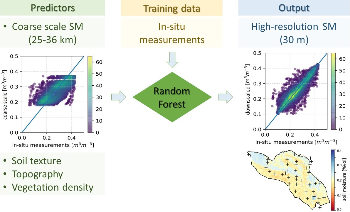
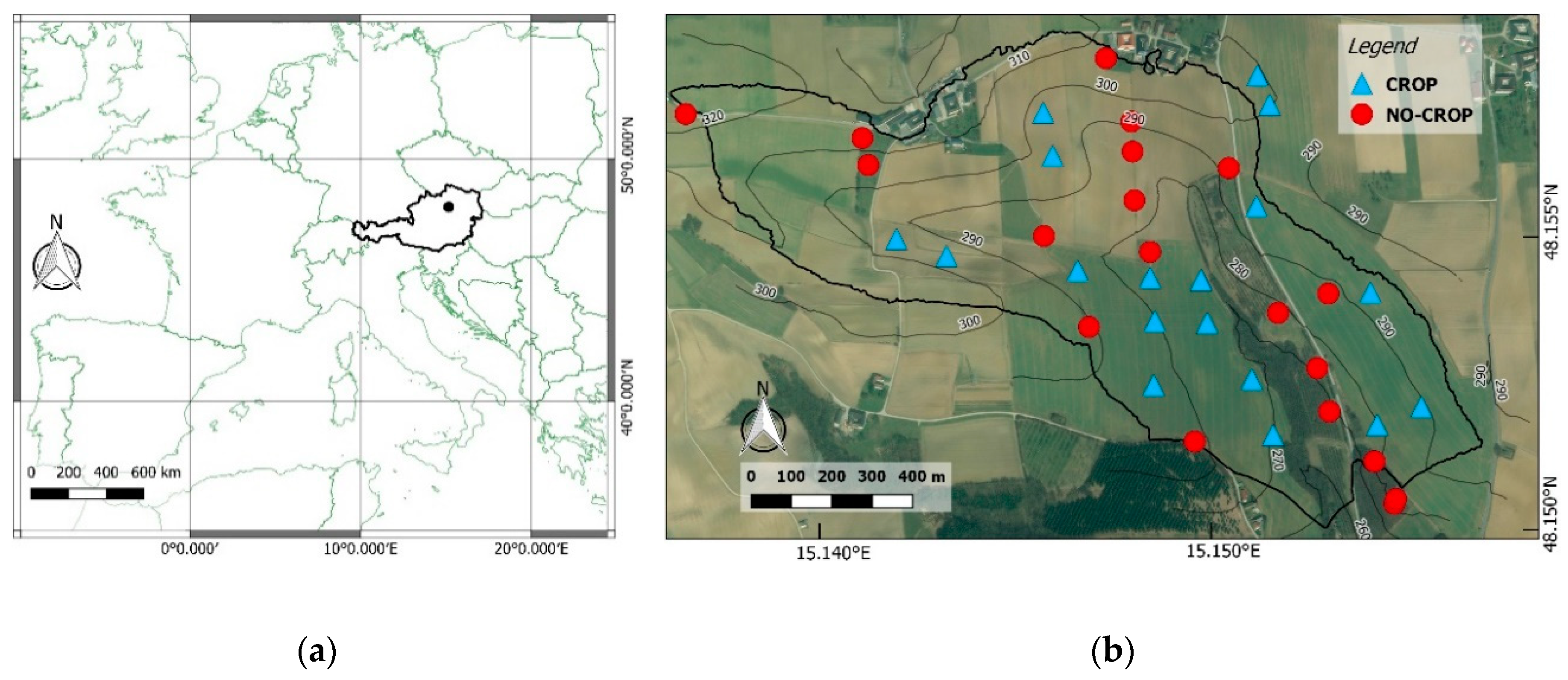
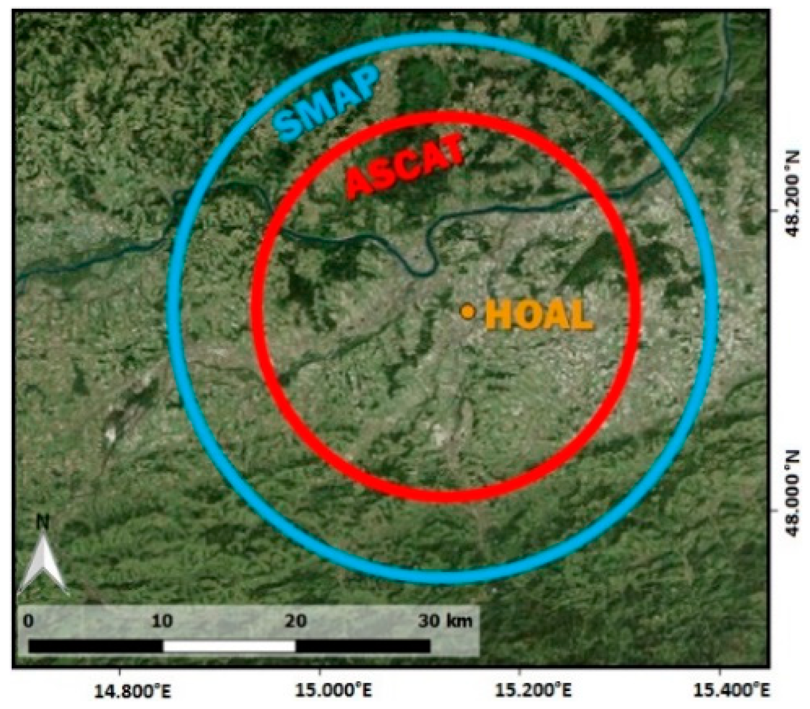
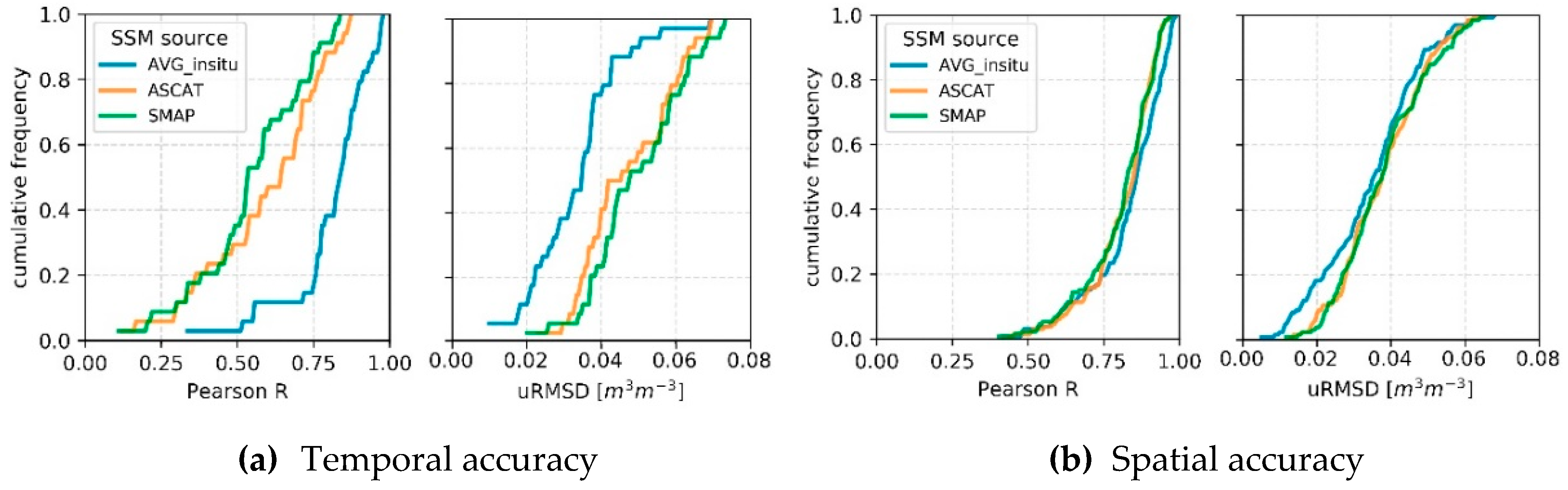
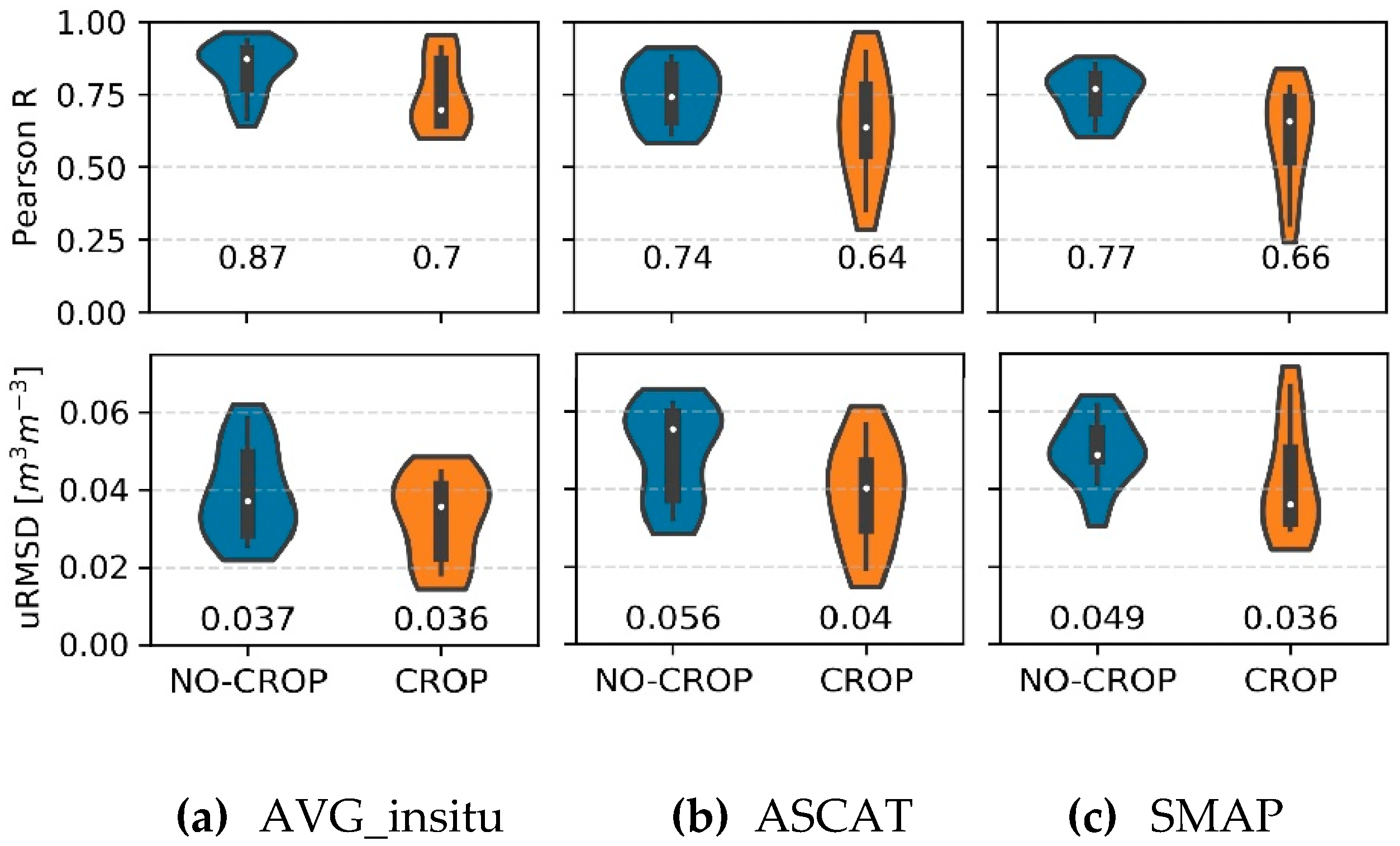
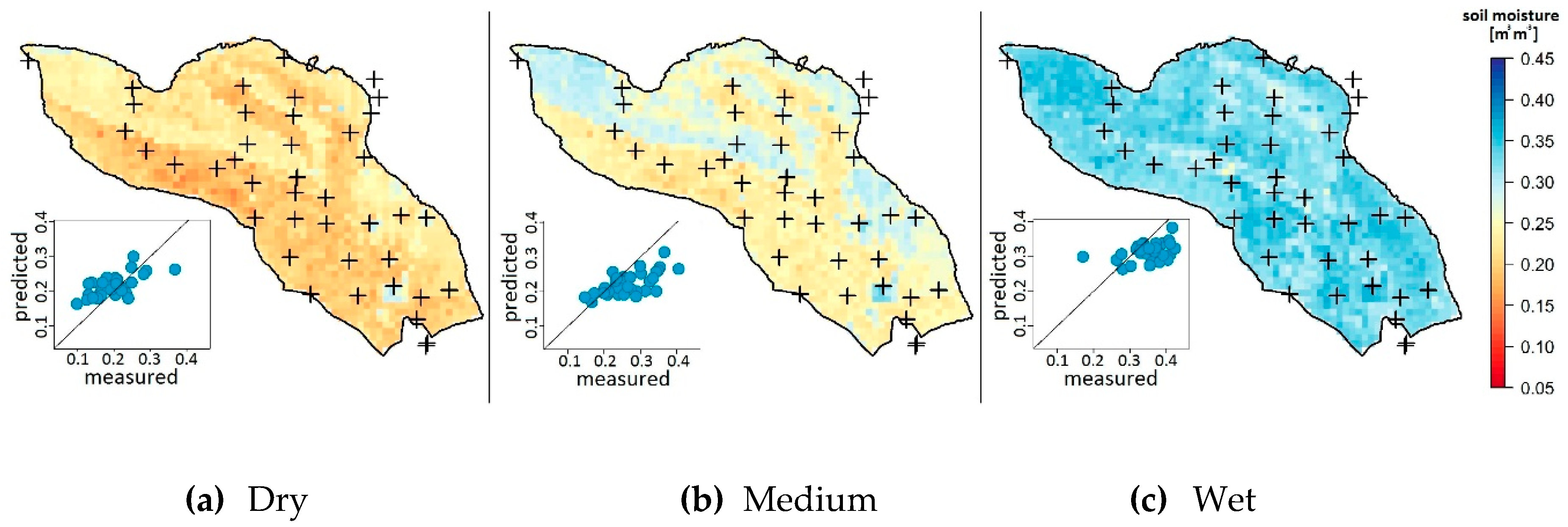
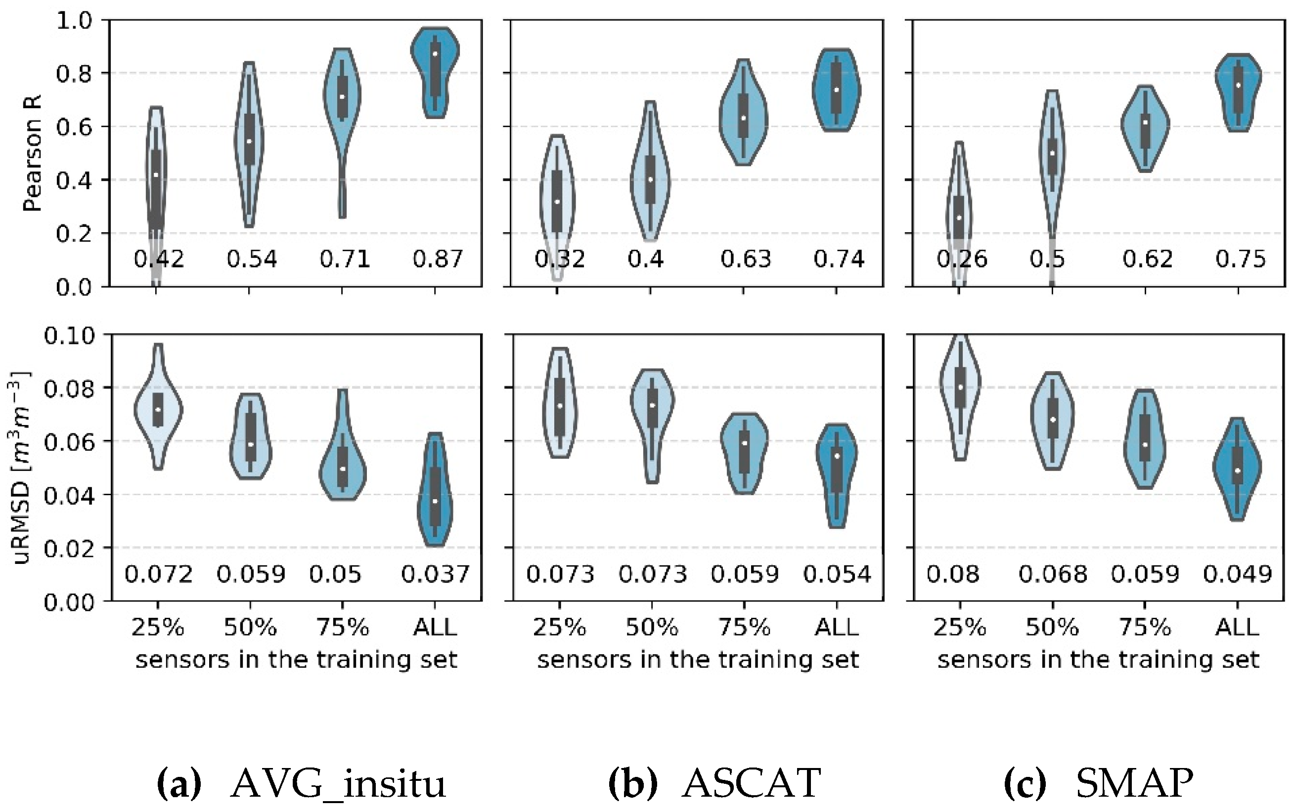
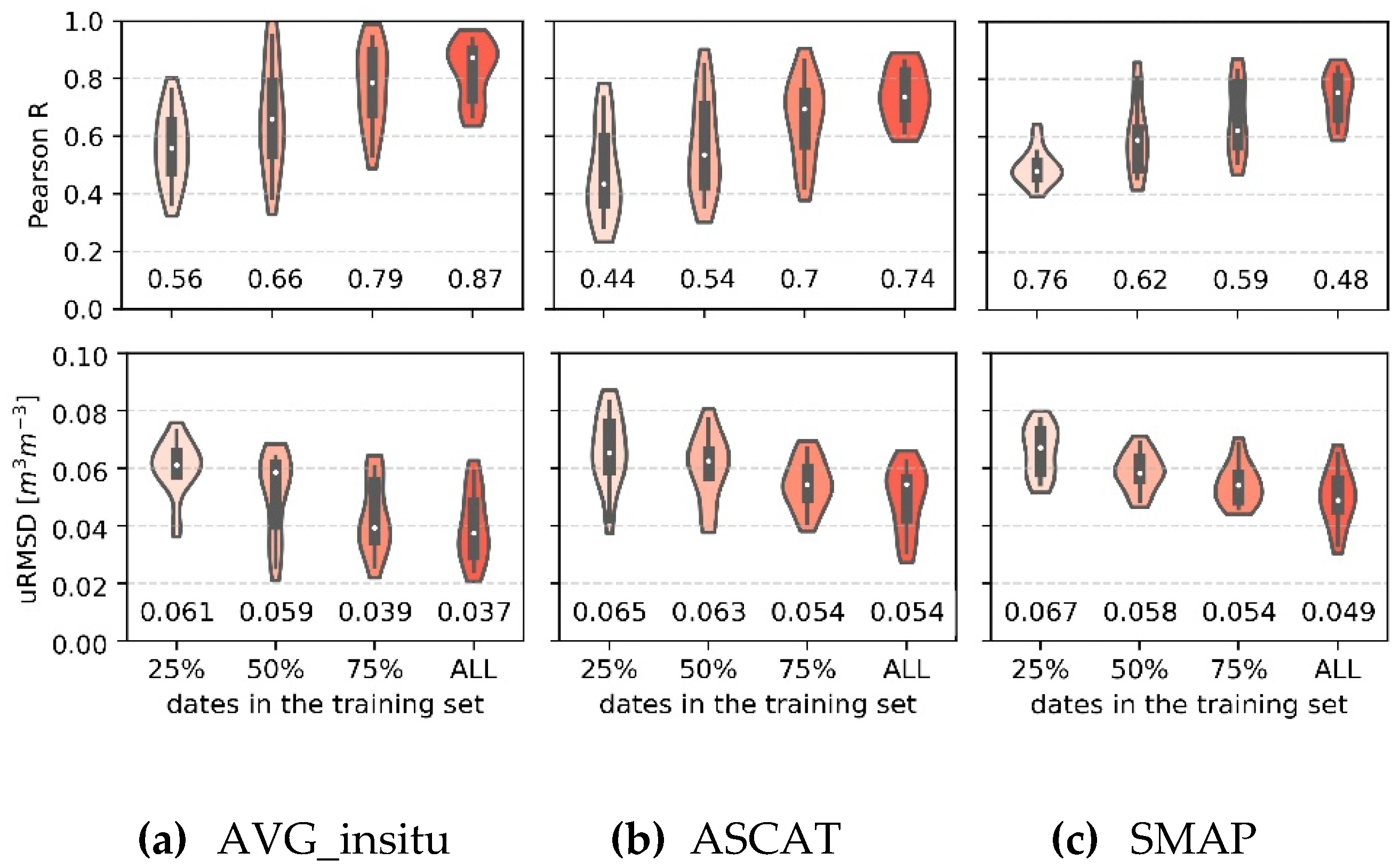
Table 1.
Summary of model combinations tested in this study.
| Predictors | |||||
|---|---|---|---|---|---|
| Coarse Scale Surface Soil Moisture (SSM) | Soil Texture (S) | Topography (T) | Vegetation (V) | ||
| Variables | AVG_insitu or ASCAT or SMAP | Clay, silt, sand | Slope, TWI, Upslope_area, Total_insolation, General_curvature | fAGR | |
| Model combinations | SSM+V | ✔ | ✔ | ||
| SSM+S | ✔ | ✔ | |||
| SSM+T | ✔ | ✔ | |||
| SSM+S+T | ✔ | ✔ | ✔ | ||
| SSM+S+V | ✔ | ✔ | ✔ | ||
| SSM+T+V | ✔ | ✔ | ✔ | ||
| SSM+S+T+V | ✔ | ✔ | ✔ | ✔ | |
© 2019 by the authors. Licensee MDPI, Basel, Switzerland. This article is an open access article distributed under the terms and conditions of the Creative Commons Attribution (CC BY) license (http://creativecommons.org/licenses/by/4.0/).
Share and Cite
MDPI and ACS Style
Zappa, L.; Forkel, M.; Xaver, A.; Dorigo, W. Deriving Field Scale Soil Moisture from Satellite Observations and Ground Measurements in a Hilly Agricultural Region. Remote Sens. 2019, 11, 2596. https://doi.org/10.3390/rs11222596
AMA Style
Zappa L, Forkel M, Xaver A, Dorigo W. Deriving Field Scale Soil Moisture from Satellite Observations and Ground Measurements in a Hilly Agricultural Region. Remote Sensing. 2019; 11(22):2596. https://doi.org/10.3390/rs11222596
Chicago/Turabian StyleZappa, Luca, Matthias Forkel, Angelika Xaver, and Wouter Dorigo. 2019. "Deriving Field Scale Soil Moisture from Satellite Observations and Ground Measurements in a Hilly Agricultural Region" Remote Sensing 11, no. 22: 2596. https://doi.org/10.3390/rs11222596
Note that from the first issue of 2016, this journal uses article numbers instead of page numbers. See further details here.