Improved Spatial-Spectral Superpixel Hyperspectral Unmixing


1
Abu Dhabi Polytechnic, Al Ain 66844, UAE
2
Electrical and Computer Engineering Department, The University of Texas at El Paso, El Paso, TX 79968, USA
*
Author to whom correspondence should be addressed.
Remote Sens. 2019, 11(20), 2374; https://doi.org/10.3390/rs11202374
Submission received: 9 September 2019
/
Revised: 7 October 2019
/
Accepted: 9 October 2019
/
Published: 13 October 2019
(This article belongs to the Special Issue Advances in Unmixing of Spectral Imagery)
Abstract
:In this paper, an unsupervised unmixing approach based on superpixel representation combined with regional partitioning is presented. A reduced-size image representation is obtained using superpixel segmentation where each superpixel is represented by its mean spectra. The superpixel image representation is then partitioned into regions using quadtree segmentation based on the Shannon entropy. Spectral endmembers are extracted from each region that corresponds to a leaf of the quadtree and combined using clustering into endmember classes. The proposed approach is tested and validated using the HYDICE Urban and ROSIS Pavia data sets. Different levels of qualitative and quantitative assessments are performed based on the available reference data. The proposed approach is also compared with global (no-regional quadtree segmentation) and with pixel-based (no-superpixel representation) unsupervised unmixing approaches. Qualitative assessment was based primarily on agreement with spatial distribution of materials obtained from a reference classification map. Quantitative assessment was based on comparing classification maps generated from abundance maps using winner takes it all with a 50% threshold and a reference classification map. High agreement with the reference classification map was obtained by the proposed approach as evidenced by high kappa values (over 70%). The proposed approach outperforms global unsupervised unmixing approaches with and without superpixel representation that do not account for regional information. The agreement performance of the proposed approach is slightly better when compared to the pixel-based approached using quadtree segmentation. However, the proposed approach resulted in significant computational savings due to the use of the superpixel representation.
1. Introduction
Hyperspectral imaging (HSI) systems collect spectral and spatial image data simultaneously in hundreds of narrow contiguous spectral bands. Hyperspectral remote sensing is used in a wide array of applications such as ecology, agriculture, mineralogy, and surveillance. In HSI, the observed radiance from a single pixel rarely comes from a pure material but from a mixture of materials in the field of view of the sensor. However, the high-spectral resolution of HSI enables the detection, identification and classification of subpixel objects by their contribution to the measured spectra. In the hyperspectral remote sensing literature, the distinct or pure materials in the scene are called endmembers, and the fractions in which they appear in each pixel are called abundances [1,2].
Hyperspectral mixing can be based on the linear mixing model (LMM) [1,2] or the nonlinear mixing model (NMM) [3]. The LMM states that the spectra of each pixel in the hyperspectral image are the convex combinations of the scene endmember. The LMM is widely used as it provides a reasonable approximation in many satellite and airborne hyperspectral remote sensing applications. The hyperspectral unmixing problem refers to finding the number of endmembers, their spectral signatures, and their per-pixel abundances in a given hyperspectral image.
Most widely used algorithms for endmember extraction are based on the relation between the LMM and convex geometry [2,4]. Because abundances are non-negative and sum to one, linearly mixed hyperspectral pixels lie inside the simplex with vertices given by the endmembers [5]. Most geometry-based endmember extraction algorithms search for the corners of the simplex as a way to extract the endmembers. The Pixel Purity Index (PPI) [5,6] algorithm projects every spectral vector onto a large set of random unit vectors (or skewers). The pixels corresponding to extremes (maximum and minimum) for the projection onto each skewer are noted. The number of times each pixel appears as an extreme point is recorded. The pixels with the highest scores are considered the purest ones and thus selected as endmembers.
N-FINDER [7] is based on the fact that, in spectral space, the volume of the simplex formed by the purest pixels is larger than the volume of the simplex generated any other combination of pixels. This algorithm finds the set of pixels defining the largest volume by inflating a simplex inside the data. First, a set of pixels are randomly selected as endmembers. The algorithm iteratively replaces every endmember for each pixel in the hyperspectral image calculating the volume. If the volume increases, then the new pixel replaces the candidate endmember.
Vertex Component Analysis (VCA) [8] is based on the fact that the affine transformation of a simplex is another simplex. VCA projects image pixels to a random direction, the pixel with the largest projection is considered the first endmember. The other endmembers are found by projecting the pixels onto a direction orthogonal to the subspace spanned by the current set of endmembers; the procedure is repeated until the whole set of endmembers is found.
The MAX-D endmember extraction algorithm [6,9] begins by finding the two pixels that are furthest apart in spectral space. All signatures are projected orthogonal to the difference vector between these two pixels, which results in these two vectors projected onto the same vector. The most distant vector from this one in the projected space is selected as the next endmember. The data are projected again orthogonal to the difference between these two vectors, and the process is repeated until the set of endmembers is extracted. PPI, N-FINDR, VCA and MAX-D assume that there are pure pixels in the image and that the number of endmembers is known.
Spatial-spectral endmember extraction approaches take advantage of spatial properties that endmembers may have for unmixing. For instance, pure endmembers in an image should be located in homogeneous areas; see, for instance, [10,11]. A survey on incorporating spatial information in spectral unmixing is presented in [12]. Another issue in spatial-spectral interaction is that there is context in the spatial distribution of materials in the image (more on that later). Some endmembers occupy small areas in the image or have low contrast with other endmembers. These signatures will be hard to extract using the geometric endmember extraction approaches described previously. Here, because of their relevance to our work, we only review spatial-spectral approaches that use spatial sub-setting to improve the detection of small and low contrast endmembers.
The Spatial-Spectral Endmember Extraction (SSEE) algorithm proposed in [13] is based on the idea that endmembers with high spectral contrast are easy to detect using any of the geometry-based techniques described previously. On the other hand, the detection of endmembers with low spectral contrast with respect to the full image is a harder task. SSEE breaks up the full image into spatial subsets increasing the relative contrast of endmembers. The singular value decomposition (SVD) is used to find a set of basis vectors that explain most of the spectral variability for the image subsets. The full image is projected onto the local basis to determine a set of candidate endmembers from where the final endmembers are selected. Spectrally similar endmembers from different spatial subsets are averaged.
The Local-Local-Global (LLG) spatially adaptive hyperspectral unmixing algorithm presented in [14] uniformly divides the image into fixed-size tiles. Endmember extraction and abundance estimation are performed on each individual tile. The Gram matrix [15,16] is used to estimate the number of endmembers on each tile. The MAX-D endmember extraction algorithm [6,9] described previously, is used for local endmember extraction on each tile. Abundances are estimated in each tile using local endmembers and spectrally similar endmembers are clustered to determine global abundances. Since the abundances are estimated locally, a tiling artifact is observed in the final abundance maps. Uniform tiling is also used in [17] for unmixing where the tiling artifact in the abundances is avoided by doing global computation of the abundances using all extracted spectral endmembers.
Another approach that uses image spatial sub-setting for unmixing is presented in [18,19], where spatial sub-setting of the image is done using quadtree partitioning (QT). The criterion for partitioning is based on entropy [20]. The constrained non-negative matrix factorization (cNMF) as proposed in [21] is used for unmixing of individual tiles. Local endmembers are clustered to form endmember classes and global abundance maps are computed by solving the global abundance estimation using all extracted endmembers to avoid the tiling artifact of the LLG algorithm in [14].
In the work presented here, we use the quadtree approach for spatial subsetting. We further explore spatial domain information in the form of superpixel representation to reduce computational complexity of the unmixing process. The proposed approach first performs superpixel segmentation using the SLIC algorithm [22]. Spatial sub-setting is then performed in the superpixel representation of the image using quadtree partitioning. The reduction in the computational complexity is a result of the unmixing process being performed on the small size superpixel representation and not in the full image as well as the low computational complexity of the SLIC algorithm (linear in the superpixel size) [22].
2. The Linear Mixing Model (LMM)
The linear mixing model (LMM) represents a pixel as the convex combination of the spectral signatures of the endmembers multiplied by its fractional area coverage (or abundance) as follows:
where is the measured spectral signature at the jth pixel, is the endmembers matrix, is the spectral abundance vector, is a noise vector, m is the number of bands, p is the number of endmembers, and N is the number of pixels.
In HSI, , elements of E, , and are constrained to be positive, and (the sum-to-one contraint). In our implementation, we will use to account for topography effects as suggested in [23,24]. For the entire HSI, the linear mixing model given above can be written in matrix form as:
where X = [] is the matrix containing all image pixels, E = [] is the matrix of endmembers, A = [] is the matrix of abundances, and W = [] is the noise matrix. Clearly, the spatial relations are not considered when unfolding the hyperspectral image into a matrix as described in Equation (2).
3. Illustrating Spatial-Spectral Interaction
Equation (2) models the full spectral data cloud as the convex hull of image endmembers. An important problem is that actual hyperspectral data clouds are not convex but better modelled piecewise-convex [25].
One cause for piecewise convexity of the hyperspectral data cloud is that materials in the scene are not uniformly distributed so certain mixtures of materials are not possible due to spatial constraints. Figure 1 illustrates this idea using simulated images that consists of a scene with three different materials distributed in two scenarios: (i) spatial random distribution with no spatial structure as shown in Figure 1a, and (ii) each material occupies a uniform spatial region as shown in Figure 1b. Figure 1c shows the spectral signatures of the materials used in the simulations. The bands used for the false-color composite were 700 nm for Red, 540 nm for Green, and 470 nm for Blue.
Figure 2 shows the scatter plots of band 80 (1.191 m) against band 196 (2.351 m). Figure 2a shows scatter plot for the first scenario (Figure 1a) where there is no spatial correlation between pixels in the scene. The image pixels are uniformly distributed inside the convex hull of the endmembers. Figure 2b shows the scatter plot for the structured scene in Figure 1b. The image pixels are distributed along two of the faces of the convex hull of the endmembers (i.e., the line between endmembers one and two and the line between endmembers two and three). Another way think of this data cloud is that the pixels are distributed in two separate simplices that is Figure 2b is piece-wise convex.
To illustrate these ideas on a real scene, we use a image chip from a 224-band AVIRIS image captured over Fort A.P. Hill, VA, USA in September of 2001 [26]. The image has 224 spectral bands from 380 to 2500 nm with a spectral resolution of 10 nm and a spatial resolution of 3.5 meters. Only 197 bands are used here for the analysis as water absorption bands (bands 107 to 114, and 153 to 167) were removed. This image chip was selected because of the way the three main classes are spatially distributed: (i) the gravel field, (ii) a grass field, and (iii) the forest region. A true-color composite is shown in Figure 3a and a scatter plot for the first two principal components in Figure 3b. The principal components are computed by, first, unfolding the hyperspectral image cube into a two-dimensional matrix, where each row contains the pixel spectral signature, then Principal Component Analysis (PCA) [27] is applied to the resulting matrix. The bands used for the color composite were 28 (635.19 nm) for Red, 19 (548.09 nm) for Green, and 10 (461.04 nm) for Blue.
Figure 3b shows the scatter plot of the first two principal components for the scene. These two principal components explain approximately 97.5% of the total scene variability. Figure 4a shows the scatter plot manually segmented into three “convex” regions. As shown in Figure 4b–d, each scatter plot segment roughly corresponds to one of the three spatial regions in the image chip. The blue region in the scatter plot represents the parking lot (Figure 4b). The green region represents the grass field (Figure 4c) and the red region represents the forest (Figure 4d). We do not have a direct way to segment the data cloud into its convex pieces in the spectral domain. Here, we propose the use of regional segmentation as a way to extract the piecewise convex structure of the data cloud.
To illustrate how spatial segmentation can be used to extract the piecewise convex structure of the data, the image is segmented using the Simple Linear Iterative Clustering (SLIC) algorithm [28] with a large region size and the resulting in coarse segments are visualized in the scatter plots shown in Figure 5. The SLIC algorithm is presented in detail in Section 4. Figure 5 shows the result of segmenting the image chip using SLIC with a region size of . The segmentation resulted in nine coarse segments. Figure 6 shows each segment and their corresponding location in the scatter plot. The spatial segmentation helps to capture parts of the piecewise convex structure of the scatter plot, but it does not produce a perfect match to the scatter plot segmentation in Figure 4. We need to be cautious in this observation as we are using a 2D scatter plot to visualize a high dimensional data set.
4. HSI Representation Using Superpixels
Most of the image processing techniques are pixel based, so, if the image is large, the computation burden will be high. Superpixel representation breaks the image into locally homogeneous regions that are not necessarily distributed in a uniform grid. Each region could be treated as a single entity during processing; since the number of superpixels will be much smaller than the number of image pixels, it results in significant computational savings. The value of the superpixel representation in image processing and computer vision has been recognized in the literature [29]. The Simple Linear Iterative Clustering (SLIC) [22] algorithm has shown better performance in superpixel segmentation than other methods in terms of computation speed and memory efficiency. SLIC is used for deriving superpixel-based representations of hyperspectral images.
SLIC starts by dividing the image into an equally spaced grid as shown in Figure 7a. The center of each grid tile is then used to initialize a k-means clustering algorithm with spatial adjacency restrictions. After clustering, SLIC optionally removes any segment whose area is smaller than a predefined threshold by merging them into larger superpixels. Figure 7b shows the final result of a segmentation. We use the SLIC algorithm for hyperspectral imagery described in [28] and the MATLAB implementation toolbox [46] provided in [30]. The work in [28] extends the standard SLIC for color images to hyperspectral images by using the full spectral signature vector and not a three-color vector as in color images.
The spectral mean:
of the spectral signatures in a superpixel is used to represent each superpixel [31,32,33]. In Equation (3), n is the number of spectral signatures in the superpixel, and is the spectral signature inside the superpixel. Each superpixel mean may represent tens to thousands of pixels in an image. Further hyperspectral image processing is performed in the superpixel means, which results in significant computational saving over full pixel-by-pixel processing. Representing the image by its superpixels can be interpreted as a non-uniform sub-sampling of the image. To illustrate the effects of superpixel representation in the spectral domain, Figure 8 shows where the mean for each superpixel is located in the scatter plot for SLIC segmentations with region size set to 25 (Figure 6) and region size set to 5. The means in Figure 8a,b are numbered based on their order of appearance in Figure 6. Centroid number 1 corresponds to Figure 6a, centroid 2 to Figure 6b and so on.
A better representation is obtained by using a smaller region size. Figure 8d,e overlays the location of the means on top of the scatter plot when the region size in the SLIC segmentation algorithm is set to 5 (). It is easy to see that the resulting means scatter plot in Figure 8d keeps most of the features of the full data scatter plot.
Another visual illustration is shown in Figure 8c,f where the true-color composite of the superpixel (SP) images for both cases are presented. A superpixel hyperspectral cube is created by arranging the mean of the SLIC superpixels to form a rectangular grid with the mean spectra of the superpixels. The color composite is formed using the same bands as in Figure 3. Figure 8c corresponds to the SP representation for the SLIC with region size parameter set to 25. The resulting SP image clearly does not preserve the spatial details of the original image (Figure 3), while the SP representation for the SLIC with region size parameter set to 5 in Figure 8f captures many of the spatial features in the original image (Figure 3). How to select an optimal superpixel size is an open question.
5. Proposed Unmixing Approach
Figure 9 depicts the proposed Unsupervised Superpixel-Based Hyperspectral Unmixing with Regional Segmentation. First, SP segmentation is applied to the image. A SP representation of the image is created by representing each superpixel by its mean spectra. Second, the SP image is partitioned into regions using quadtree segmentation. Endmember extraction is applied to each region associated with a tree leaf to extract regional spectral endmembers. Extracted spectral endmembers are clustered into endmember classes. Abundances are computed over the full image using the extracted spectral endmembers. The abundance for and endmember class is the sum of the abundances of the individual spectral endmembers belonging to it.
5.1. Quadtree Regional Segmentation
The SP image is divided into spatial regions for unmixing using quadtree partitioning. The spatial subsetting, as mentioned previously, makes the approach more sensitive to low contrast or small endmembers present in small regions. Figure 10 illustrates the basic idea of quadtree segmentation.
The image is first divided into four equally sized tiles and the Shannon entropy is computed for each tile. The Shannon entropy for a tile R is given by:
where T is the number of clusters in R, and is the ratio between the number of pixels in cluster i to the total number of pixels in R. If the entropy for the resulting tiles is higher than 90% of the global entropy, the tile is divided again into four equally sized tiles [20]. The process is continued until the resulting tile has an entropy lower than 90% of the global entropy or the tile size reaches a minimum size (8 × 8 in our case). The leaves of the tree are the regions used in subsequent analysis.
5.2. Endmember Extraction
After quadtree partitioning, the next step is to extract the endmembers from each leaf tile. The first step is to determine the number of endmembers since most endmember extraction methods assume that it is known.
5.2.1. Estimating the Number of Endmembers
The rank of the Gram Matrix [34] is proposed in [15,16] as a way to estimate the number of endmembers. The Gram Matrix G of a set of vectors is given by
G is an matrix. Note that the element of the Gram Matrix is given by , the inner product between vectors , . A useful property of the Gram Matrix for unmixing is that its determinant, the Grammian, is the square of the volume of the parallelepiped formed by the vectors of Y [35]. In addition, the vectors are linearly independent if and only if the Grammian is nonzero or, equivalently, the rank of G is equal to the rank of Y.
In [15,16], the matrix Y is constructed from sample pixels from the hyperspectral image sorted in descending order of magnitude. The sample of pixels in Y can selected using geometric endmember extraction techniques, where m is an overestimate of the number of endmembers.
The submatrix G (using MATLAB notation) is the leading principal submatrix of G[34]. The leading principal minor is the determinant of a leading principal submatrix. In [15,16], the leading principal minors of the Gram Matrix starting with are computed for or until the determinant reaches zero. Typically, the magnitude of the principal minors peaks at a small values of k and then monotonically decreases. The value of k where the peak happens is used as the estimate of the number of endmembers.
5.2.2. Endmember Extraction Using SVDSS
Endmember extraction will be performed on each leaf of the quadtree using the Singular Value Decomposition Subset Selection (SVDSS) method. SVDSS is an algorithm used to select the most independent subset of columns from a matrix [36]. It has been applied to band subset selection in the past [37].The use of SVDSS for endmember extraction was proposed in [38]. Given p, the number of endmembers, the endmember signatures are extracted using SVDSS as follows:
- Unfold the hyperspectral image cube (3D-array) into a matrix representation , where each column of X corresponds to the spectral signature of each image pixel, and N is the number of pixels.
- Compute the first p right singular vectors of X, .
- Let XP = [], where and . will be the matrix of endmembers
It is shown in [38] that SVDSS tends to choose vectors with a large simplex volume.
5.3. Endmember Class Extraction
Spectral endmembers from individual tiles are clustered into groups with similar spectral signatures. These clusters represent the distinct materials in the image, and the clustering captures their variability across the scene. The clusters of spectral endmembers are called spectral endmember classes.
In the proposed approach, the cosine distance is used as the similarity measure for clustering:
If , the endmembers belong to the same spectral endmember class. The principal advantage of this clustering approach is that it does not need a specific number of clusters. We used the clustering command from the statistics toolbox [39] available in MATLAB to perform the clustering analysis.
5.4. Abundance Estimation
Once the endmember classes are determined, the next step is to estimate their abundances. The abundances are computed by solving the following constrained linear least squares problem
where the endmember matrix E includes all spectral endmembers. The reason for using (NNSLO) constraint instead of the (NNSTO) constraint is to account for topography effects as described in [40]. The abundance of an endmember class is the sum of the abundances of the spectral endmember signatures belonging to that class. We use the implementation of [40] to solve (7).
6. Experimental Results
This section presents experimental results evaluating the performance of the superpixel-based unmixing with regional segmentation approach using real hyperspectral image data sets. In Section 6.2, we compare our approach using quantitative and qualitative analysis with other approaches used in the literature.
6.1. Data Sets
Two hyperspectral images were selected for the experiments: HYDICE Urban and ROSIS Pavia University. These images were selected because of the availability of reference data in the format of published spectral libraries and classification maps used later for indirect assessment of unmixing results.
6.1.1. HYDICE Urban Data Set
HYDICE Urban is a widely used hyperspectral data set used in unmixing studies. It was collected with the Hyperspectral Digital Image Collection Experiment (HYDICE) sensor in October 1995. The scene is an urban area at Copperas Cove, TX, USA [41]. The scene has pixels at 2 m resolution, and 210 bands between 400 nm to 2500 nm at a spectral resolution of 10 nm. After channels 1–4, 76, 87, 101–111, 136–153 and 198–210 are removed (due to dense water vapor and atmospheric effects), we end with 162 channels for processing. The data are already calibrated to reflectance. Figure 11a presents a true-color composite using band 28 (680 nm) for red, band 14 (540 nm) for green, and band 7 (470 nm) for blue. A reference from [42] shown in Figure 11b is used here as a reference classification map. The classification map shows five information classes: Asphalt, Grass, Tree, Roof and Soil (Dirt). An endmember spectral library is also available from [42] and is shown in Figure 11c. The reference data also include abundance maps for these classes, and we will use them later for algorithm assessment.
6.1.2. ROSIS Pavia University
This is a scene acquired with the ROSIS sensor during a flight campaign over Pavia, northern Italy. The image consists of 103 spectral bands from 430 to 860 nm with a spectral resolution of 4 nm and a spatial resolution of 1.3 m. Only 103 bands are used for the unmixing analysis. Pavia University is pixels. Figure 12a shows a true color composite of the scene. The reference classification map for the Pavia University scene is shown in Figure 12b. The classification map shows nine classes: Asphalt, Meadows, Gravel, Trees, Metal Sheet, Bare Soil, Bitumen, Brick and Shadow. The unassigned pixels in the image are colored in black and labeled as “background”. Figure 12c shows the endmembers for the labeled samples.
6.2. Assessment Approach
A problem with assessing the performance of unmixing algorithms is the lack of data sets with abundance reference data. Typical data sets such as Fort A.P. Hill, HYDICE Urban, ROSIS Pavia, and others have documented classification maps and spectral libraries. The lack of abundance information becomes a limitation to directly assess unmixing results.
Typically endmember extraction results are evaluated by computing the spectral angle between the extracted endmember signatures and reference spectra. Unmixing results are indirectly assessed using the reconstruction error between the image reconstructed from the estimated abundances and extracted endmembers and the original image [43]. However, the reconstruction error only assesses the fitting error but not the accuracy of the estimated abundance maps or endmembers.
Here, we will follow the assessment methodology described in [44] based on the agreement matrix (similar to the error or confusion matrix in classification) between the generated class map and the reference classification map. We will also perform visual comparison between abundance maps and individual binary class maps. This helps us assess whether or not we are extracting the right spatial distribution of the information classes. Note that information classes in the classification maps may correspond to multiple endmember classes. In the case of the HYDICE Urban image, there are reference abundance maps from [41], which allow for a more quantitative comparison. However, there is no information on the accuracy of these reference abundances in [41]. We will still compare derived and reference abundance maps in what follows.
A classification map can be derived from the abundance maps by assigning the pixel to the endmember class with the highest abundance (i.e., winner takes all). We use a winner takes all strategy that also requires that the maximum abundance meets a minimum threshold of 50% and the pixel remains unassigned if not. Once the class map is derived, quantitative methods such as agreement matrices and kappa statistics are used to assess the pixel-by-pixel agreement between the two classification maps [6,44,45]. Notice that we are not assessing the agreement of the classification map with ground truth but with a reference classification map.
Comparing Generated and Reference Maps
The agreement matrix is computed by using a pixel by pixel comparison between the derived and reference maps. Four statistics are computed from the agreement matrix motivated by the error matrix in pattern recognition: (1) the Producer’s Agreement refers to the probability that a certain land-cover of an area on the reference map is assigned the same class in the generated map, (2) the User’s Agreement which is the probability that a pixel labeled as a certain land-cover class in the generated map has the same assignment in the reference map, (3) the Overall Agreement that indicates the percentage of pixels with the same label in both the reference and the generated classification maps, and (4) Cohen’s kappa coefficient [45]. The kappa statistic is a more robust measure than simple percentage agreement calculation, as it takes into account the possibility of the agreement occurring by chance. It measured the agreement between the two maps.
6.3. Experimental Results for the Urban Data Set
First, superpixels (SP) were extracted using the SLIC algorithm with a region size of ; this particular size was selected based on the work by [28]. The result was a nearly grid of superpixels (a total of 394 superpixels since very small superpixels were merged with larger ones). The SLIC segmented image is shown in Figure 13a.
For each superpixel, the spectral mean of the spectral signatures is calculated. Although the SLIC image has a non-uniform spatial arrangement of superpixels, each SLIC superpixel initial starting point was on a uniform grid (see Figure 7). For the purpose of visualization, we assign the mean of the final superpixel to the location of the superpixel initial location. We accept that this visualization has some limitations but helps us in understanding and implementing the approach. The result is an image cube of size shown in Figure 13b. Locations of small superpixels that were merged with larger ones will be given no value (blank pixels using NaN in MATLAB). Those “empty” pixels will not be included in any further processing.
The SP representation cube is partitioned using the quadtree method. The result of the partitioning is shown in Figure 13c. The Gram matrix method is used to estimate the number of endmembers in each tile. The results are also shown in Figure 13c.
Endmember extraction is performed on each tile on the leaves of the quadtree using SVDSS; a total of 45 endmembers were extracted and are shown in Figure 14. The extracted spectral endmembers were clustered using the cosine distance with a threshold of 0.005. The clustering analysis resulted in 17 endmember classes. Finally, abundance estimation using NNSLO [40] was performed using the 45 endmembers over the whole image. The abundance for each class is the sum of abundances for the spectral endmembers belonging to the endmember class. The pixel abundances are normalized to sum to one in a post-processing step.
Abundance maps and spectral signatures from endmember classes are manually grouped to correspond to information classes based on the classification map. Figure 15 and Figure 16 show the spectral endmember signatures that are assigned to an information class and the resulting combined abundance maps. The abundance map for an information class is the sum of the abundances for the endmembers classes belonging to that information class.
6.3.1. Qualitative Assessment
The evaluation of unmixing results is performed by comparing extracted information endmember classes and estimated abundances with published spectral libraries and classification maps for the HYDICE Urban image. Figure 17 presents a comparison between the information abundance maps extracted from the Urban scene using the proposed approach (Top row) and the reference abundance maps (Second row) obtained from [42]. The absolute value of the difference between these abundance maps is shown in the third row and its histogram in the fourth row. The first column is the Asphalt/Road class. The second is the Grass class. The third is the Trees class. The fourth is the Roof class. The fifth column is the Soil class.
Based on these results, we can see that there is good agreement between the reference and estimated abundances for the Trees and Grass classes, followed by Asphalt/Road, Soil and Roof. Furthermore, we can argue that we do a better job in extracting the Roof and the Asphalt/Road classes compared to the reference data based on visual comparison between our abundance maps and the image.
Extracted and reference spectral signatures are shown in Figure 18. The endmember shapes are comparable for all except the roof class where some of the extracted spectral endmembers do not match well the reference data. The same could be said to some extend to the the Dirt class. We feel that the spectral variability of the classes is better captured by the endmember classes than by a single spectral signature as in the the reference data. We feel that capturing this variability is what allows us to get better results in the roof class.
6.3.2. Quantitative Assessment
For quantitative analysis, a classification map is generated from the abundance maps using a winner takes it all approach with a 50% threshold. The resulting classification map and the reference map are compared using the agreement matrix. Four statistics are computed: Producer’s agreement (PA), User’s agreement (UA), Overall agreement (OA) and the Cohen’s kappa [45]. The harmonic mean (HM) is used to assess the per-class agreement as it balances the UA and PA rates. It is given by
Furthermore, the spatial post-processing step using a median filter is used to clean scattered individual miss-classified pixels from the resulting class. The assumption is that information classes will occupy relatively uniform spatial areas (larger than just a few pixels). Median filtering produces a smoother version of the class map. The smoothed classification map is compared to the reference map using the agreement matrix.
Figure 19 shows the classification maps for the Urban scene. Figure 19a shows the classification map generated from the estimated abundances. Figure 19b shows the classification map from Figure 19a after being smoothed with the median filter. Figure 19c shows the reference data classification map. Table 1 presents the agreement matrix between the generated classification map and the reference. Table 2 shows the agreement matrix between the filtered generated classification map and the reference. The un-assigned class in the tables refer to pixels that did not meet the more than 50% criteria in the majority vote assignment.
The generated classification map has an overall agreement of 79.51% with the reference map. Individual classes have a producer’s agreement higher than 75%. In the user agreement, accuracies for Trees, Grass, and Road are above 85%, while, for Dirt and Roof, they are below 65%. These differences are captured in the harmonic mean that for Trees, Grass, and Road are above 80% while for Dirt and Road are below 70%. In the resulting class map, many Grass pixels are classified as Trees, while Trees and Road are classified as Roof. Grass and Dirt coexist and are mixed in multiple areas of the image so this confusion is not surprising. This is similar for Trees and Road and Roof. The reference data do not provide accuracy data for the reference map. In addition, as mentioned earlier, we think our approach does a better job in extracting the abundances in the residential areas on the left half of the image where most roofs, trees and soil related pixels are located. In the end, the final assessment was the Cohen’s kappa score, which was 73.06%, and this indicates a substantial agreement between the two maps based on [45].
The analysis using the agreement matrix is also performed on the median filtered classification map shown in Figure 19b. Table 2 shows the agreement matrix between the filtered generated classification map and the reference map. The overall agreement increases by over 9%. The harmonic mean increases for Trees, Grass, and Road, and it is still above 87% for all these classes. The harmonic mean increases for Dirt and Road by at least 9%. This is primarily due to an increase in UA, which for Dirt was 26%, while, for Roof, it was 9%. The kappa coefficient for the agreement is 84.43%, which indicates an almost perfect agreement between the two maps [45].
6.4. Experimental Results for the Pavia University Data Set
The proposed unmixing approach is also used to analyze the Pavia University data set. An SP representation is derived using SLIC with region size of . The resulting SP representation was a grid of superpixels as shown in Figure 20a.
The spectral means of the SP are used to derive a reduced-size image cube representation of size shown in Figure 20b. The results of the SP cube partitioning using the quadtree approach are shown in Figure 20c. The estimated number of endmembers using the Gram method is also shown.
Endmember extraction is performed on each tile using SVDSS (see Figure 21 for results). A total of 58 endmembers were extracted. The extracted spectral endmembers were clustered using the cosine distance with a threshold of 0.005. Clustering analysis resulted in 20 spectral classes. Finally, abundance estimation using NNSLO [40] was performed using the 58 endmembers over the whole image. The abundance for each class is the sum of abundances for the spectral endmembers belonging to the class. A post-processing step is to normalize the abundance maps to sum to one as discussed previously.
Endmember classes are manually combined to match information classes in the classification map as we did in the Urban example. By looking at Figure 22a, we can see that Gravel and Brick classes have similar spectra, and similarly Asphalt and Bitumen. Thus, for our analysis, we decided to combine both Gravel and Brick to form a single information class, and Asphalt with Bitumen into another information class. Figure 23 and Figure 24 show the information classes endmembers and their corresponding abundance maps.
By further studying the true-color composite of the scene and comparing with the class map (Figure 12), some regions classified as Meadows look like Bare Soil (see Figure 22b). In addition, the spectral signatures for these two classes are quite similar as well; see Figure 12. Both information classes were merged together to form a single information class for our analysis as well.
6.4.1. Qualitative Assessment
For the Pavia scene, the reference data did not include abundance maps but only a classification map. Therefore, we are not able to perform the type of comparison shown in Figure 18 for the Urban data set. Here, extracted abundance maps for the Pavia data set are visually compared to binary class maps from the reference classification map. Figure 25 shows the extracted abundance map and the reference binary class map for the Asphalt-Bitumen class. Note that the binary class map covers areas contained in the abundance map. A portion of the road in the abundance map does not appear in the reference class map. By looking at Figure 12b, this part was considered as a background (not assigned) in the reference map. Our approach successfully captures the entire road in the scene, which can be confirmed from visual inspection of the true-color composite for the scene shown in Figure 12a).
Figure 26 shows similar results for the Meadows-Bare Soil class. The abundance map includes the reference binary map as before as well as multiple regions that were not assigned in the reference map and labeled background. Similar results can be shown for the other four classes as shown in Figure 27.
6.4.2. Quantitative Assessment
Figure 28 shows the classification maps for the Pavia scene. Figure 28a shows the classification map generated from the abundance maps using majority voting and the 50% threshold. Figure 28b shows the classification map after smoothing with a median filter. Figure 28c shows the reference data classification map after merging spectrally similar information classes as discussed previously. In the computation of the agreement matrix, pixels labeled as background in the reference data were not included. Table 3 presents the agreement matrix for Figure 28a, while Table 4 shows the agreement matrix for Figure 28b.
The generated map has an overall agreement of 73.59% with the reference map (see Table 3). The kappa coefficient is 62.10%, which indicates a substantial agreement [45] between the two maps. The harmonic mean was over 60% for all classes but the Shadow class, which means that there is a good agreement between the generated and reference maps for those classes. The Asphalt and Bitumen and Shadow classes have a relatively low producer’s agreement (less than 50%). Many of the Asphalt and Bitumen pixels were un-assigned based on the abundance threshold of 50% that generates the class map that dropped the producer’s agreement significantly. The Trees class was heavily confused with the Meadows-Bare Soil class. Close to a third of the Trees class pixels were classified as Meadows and Soil class. Close to a quarter of the pixels classified as Trees were from Meadows-Bare Soil. The spectral signature of these classes are very similar and most of the Trees pixels are scattered in the image and mixed with other classes.
The filtered classification map has an overall agreement of 79.80% (Table 4), which is higher by 6% than the unfiltered map. The harmonic mean did not change significantly for most classes with the exception of Shadow, where it went down from 55.05% to 47.90% reducing significantly the agreement for that class. This is not surprising, as this is a small class and median filtering will eliminate pixels in this class. The harmonic mean Trees increased slightly by 3%. Although the user’s agreement Trees increased by almost 15%, the producer’s agreement decreased by more than 4%. A larger number of Trees were classified as Meadows and Soil than for the previous map. The kappa coefficient has a value of 69.30%, which is better than the previous one.
7. Comparing with Other Methods
This section presents a comparison of the proposed approach results with other approaches. We first compare with global analysis where there is no use of spatial subsetting. The full hyperspectral image is used for endmember extraction with no spatial subsetting or SP segmentation (Full Global). The second comparison is with global unmixing over the SP image. Here, endmember extraction is performed over the entire SP representation with no spatial subsetting (SP Global). The third comparison is with spatial subsetting of the full hyperspectral image using quadtree partitioning. The full hyperspectral image is partitioned in spatial regions using quadtree segmentation and endmember extraction is performed on each leaf of the quadtree (Full + QT). This is similar to the approach for unmixing with the cNMF described in [19]. For all approaches, the number of spectral endmembers is estimated using the Gram method. Abundances are computed using NNSLO and manually grouped according to the information classes from the reference map. Comparisons will be presented only for the Urban scene based on the agreement matrix.
The Gram method estimated 16 spectral endmembers for the full hyperspectral image and 10 for its full SP representation with no quadtree partitioning. Endmembers were extracted using SVDSS and abundances estimated with NNSLO. Spectral endmember abundances were manually grouped into information classes by visual comparison with the reference map. The resulting abundance maps for the information classes are shown in the first two rows from top to bottom in Figure 29 and the corresponding spectral signatures in Figure 30.
Quadtree segmentation was applied to the full hyperspectral image, and the number of spectral endmembers was determined for each tile using the Gram approach. Figure 31a shows the results of the quadtree segmentation and Figure 31b shows the number of spectral endmembers per tile (total of 114). Endmembers were extracted using SVDSS. Abundance estimation using the NNSLO is applied to the full image using the extracted spectral endmembers. Clustering using the angle distance with a threshold of 0.005 led to 30 endmember classes. Endmember classes were manually grouped into information classes by visual comparison with the reference data. The resulting abundance maps for the information classes are shown in the third row from top to bottom in Figure 29. The corresponding information class spectral signatures are shown in Figure 30.
By visually comparing the spectral signatures extracted using the global method to the ones available from the reference data (Figure 30), the extracted endmembers do not look similar to the reference data in terms of shape. This is easily noticed for the Road class, while, when comparing the endmembers obtained from the Global SP approach to the reference data, there is a better similarity in terms of shape (except for the road and roof classes).
A class map is generated for each approach based on the abundance maps from Figure 29 using a winner takes it all with a 50% threshold criteria. The resulting class maps are shown in Figure 32. Pixels with the black label in the map are those where the winner did not have more than 50% abundance. Each generated class map in Figure 32 is compared to the reference data using the agreement matrix. The corresponding agreement matrices are shown in Table 5, Table 6 and Table 7.
Table 8 shows a comparison of the harmonic means, overall agreements and kappa statistic for all four approaches. The proposed approach (SP + QT) has the closest agreement with the reference data as shown by the highest harmonic means, highest kappa and highest overall agreement (All shown in bold). This means it has an overall better per-class agreement than the other methods. In addition, when comparing Table 2 and Table 7, we can see that the proposed approach has higher producer agreement rates than Full+QT for all classes except Road. In user agreement, Full + QT has lower agreement rates for Road and Grass. The results do point to significant differences between SP + QT and Full + QT. Full + QT is significantly more computationally demanding than SP + QT. The endmember extraction stage comprised of quadtree segmentation and application SVDSS to the tree leaves when performed on the full image requires processing pixels, while, for the SP representation, we only need to process 394 superpixels. The additional overhead for SP segmentation and the computation of the means are lower than the quadtree segmentation. Abundance computation uses NNSLO applied to all pixels in both approaches.
8. Conclusions
This work proposed a new spatial-spectral approach for unmixing analysis using superpixel representation combined with quadtree segmentation. A reduced size hyperspectral image representation is obtained using superpixel segmentation where each superpixel is represented by its mean spectra. Regional analysis is then performed using the quadtree segmentation based on Shannon entropy. Endmembers are extracted from each region and combined using clustering into endmember classes based on the spectral angle distance.
Experimental analysis of the unsupervised unmixing approach was conducted using real hyperpectral imagery from HYDICE and ROSIS sensors. It is important to recognize that there are limitations to perform quantitative assessment of unmixing results. Most of the time, only classification maps and spectral libraries are available as reference data. The assessment methodology in this paper was based on comparing derived classification maps from abundance maps with reference maps using the agreement matrix. To make this comparison possible, abundance maps for endmember classes are grouped manually to correspond to information classes in the reference classification map.
The quantitative assessment is performed using four statistics: Producer’s agreement, User’s agreement, Harmonic mean, Overall agreement and kappa statistic. The proposed unmixing approach obtained good results (high harmonic means) for most of the Urban and Pavia classes. The kappa statistic was over 80% for both data sets indicating an almost perfect agreement between the derived map and the reference data.
The proposed approach was also compared with global endmember extraction (no spatial subsetting) with the full image and the SP representation, and with spatial subsetting applied to the full image. Results show that the proposed approach does better than global approaches that do not use spatial subsetting while results are comparable to those of the quadtree approach applied to the full image. However, the proposed approach has much lower computational requirements since the analysis is done on the SP representation instead of the full image and the additional overhead of SLIC segmentation and mean computation is lower than that for quadtree partitioning over the entire image.
The proposed approach has been shown to have great potential for improved hyperspectral unmixing. Furthermore, the idea of using an SP pixel representation to improve computational speed was also shown in [28]. However, the problem of automatically finding the optimal SP size is still an open problem that requires further attention. A small value might lead to high over-segmentation of the image where the size reduction brought by the SP representation is lost, while having a high region size will result in non-homogeneous superpixels and a poor representation of the image.
Author Contributions
Conceptualization, M.Q.A. and M.V.-R.; methodology, M.Q.A. and M.V.-R.; software, M.Q.A.; validation, M.Q.A. and M.V.-R.; formal analysis, M.Q.A. and M.V.-R.; investigation, M.Q.A. and M.V.-R.; resources, M.Q.A.; data curation, M.Q.A.; writing—original draft preparation, M.Q.A.; writing—review and editing, M.Q.A. and M.V.R.; visualization, M.V.-R.; supervision, M.V.-R.; project administration, M.V.-R.; funding acquisition, M.V.-R.
Funding
This research was supported in part by the Texas Instruments Foundation Endowed Scholarship Program for graduate students in Electrical and Computer Engineering at the University of Texas at El Paso. Dr. Velez was partially supported by US Army Research Office (ARO) under award W911NF1910011.
Conflicts of Interest
The authors declare no conflict of interest.
References
- Keshava, N.; Mustard, J.F. Spectral unmixing. IEEE Signal Process. Mag. 2002, 19, 44–57. [Google Scholar] [CrossRef]
- Parente, M.; Plaza, A. Survey of geometric and statistical unmixing algorithms for hyperspectral images. In Proceedings of the 2nd Workshop on Hyperspectral Image and Signal Processing: Evolution in Remote Sensing (WHISPERS), Reykjavik, Iceland, 14–16 June 2010; pp. 1–4. [Google Scholar]
- Heylen, R.; Parente, M.; Gader, P. A review of nonlinear hyperspectral unmixing methods. IEEE J. Sel. Top. Appl. Earth Obs. Remote Sens. 2014, 7, 1844–1868. [Google Scholar] [CrossRef]
- Keshava, N. A survey of spectral unmixing algorithms. Linc. Lab. J. 2003, 14, 55–78. [Google Scholar]
- Boardman, J.W. Automating spectral unmixing of AVIRIS data using convex geometry concepts. In Proceedings of the Summaries of the 4th Annual JPL Airborne Geoscience Workshop, Washington, DC, USA, 25–29 October 1993; Volume 1, pp. 11–14. [Google Scholar]
- Schott, J.R. Remote Sensing: The Image Chain Approach; Oxford University Press on Demand: Oxford, UK, 2007. [Google Scholar]
- Winter, M.E. N-FINDR: An algorithm for fast autonomous spectral end-member determination in hyperspectral data. Proc. SPIE 1999, 3753, 266–276. [Google Scholar]
- Nascimento, J.M.; Dias, J.M. Vertex component analysis: A fast algorithm to unmix hyperspectral data. IEEE Trans. Geosci. Remote Sens. 2005, 43, 898–910. [Google Scholar] [CrossRef]
- Schott, J.R.; Lee, K.; Raqueno, R.; Hoffmann, G.; Healey, G. A subpixel target detection technique based on the invariance approach. In Proceedings of the 12th JPL Airborne Earth Science Workshop, Pasadena, CA, USA, 25–28 February 2003; pp. 241–250. [Google Scholar]
- Plaza, A.; Martínez, P.; Pérez, R.; Plaza, J. Spatial/spectral endmember extraction by multidimensional morphological operations. IEEE Trans. Geosci. Remote Sens. 2002, 40, 2025–2041. [Google Scholar] [CrossRef] [Green Version]
- Torres-Madronero, M.C.; Velez-Reyes, M. Integrating spatial information in unsupervised unmixing of hyperspectral imagery using multiscale representation. IEEE J. Sel. Top. Appl. Earth Obs. Remote Sens. 2014, 7, 1985–1993. [Google Scholar] [CrossRef]
- Shi, C.; Wang, L. Incorporating spatial information in spectral unmixing: A review. Remote Sens. Environ. 2014, 149, 70–87. [Google Scholar] [CrossRef]
- Rogge, D.M.; Rivard, B.; Zhang, J.; Sanchez, A.; Harris, J.; Feng, J. Integration of spatial–spectral information for the improved extraction of endmembers. Remote Sens. Environ. 2007, 110, 287–303. [Google Scholar] [CrossRef]
- Canham, K.; Schlamm, A.; Ziemann, A.; Basener, B.; Messinger, D. Spatially adaptive hyperspectral unmixing. IEEE Trans. Geosci. Remote Sens. 2011, 49, 4248–4262. [Google Scholar] [CrossRef]
- Messinger, D.W.; Ziemann, A.K.; Schlamm, A.; Basener, W. Metrics of spectral image complexity with application to large area search. Opt. Eng. 2012, 51, 036201. [Google Scholar] [CrossRef]
- Messinger, D.; Ziemann, A.; Schlamm, A.; Basener, B. Spectral image complexity estimated through local convex hull volume. In Proceedings of the 2nd Workshop on Hyperspectral Image and Signal Processing: Evolution in Remote Sensing (WHISPERS), Reykjavik, Iceland, 14–16 June 2010; pp. 1–4. [Google Scholar]
- Goenaga, M.A.; Torres-Madronero, M.C.; Velez-Reyes, M.; Van Bloem, S.J.; Chinea, J.D. Unmixing analysis of a time series of Hyperion images over the Guánica dry forest in Puerto Rico. IEEE J. Sel. Top. Appl. Earth Obs. Remote Sens. 2012, 6, 329–338. [Google Scholar] [CrossRef]
- Goenaga-Jimenez, M.A.; Velez-Reyes, M. Incorporating local information in unsupervised hyperspectral unmixing. Proc. SPIE 2012, 8390, 83901N. [Google Scholar]
- Goenaga-Jimenez, M.A.; Velez-Reyes, M. Integrating spatial information in unmixing using the nonnegative matrix factorization. Proc. SPIE 2014, 9088, 908811. [Google Scholar]
- Goenaga-Jimenez, M.A.; Velez-Reyes, M. Comparing quadtree region partitioning metrics for hyperspectral unmixing. Proc. SPIE 2013, 8743, 87430Z. [Google Scholar]
- Masalmah, Y.M.; Velez-Reyes, M. A full algorithm to compute the constrained positive matrix factorization and its application in unsupervised unmixing of hyperspectral imagery. Proc. SPIE 2008, 6966, 69661C. [Google Scholar]
- Achanta, R.; Shaji, A.; Smith, K.; Lucchi, A.; Fua, P.; Süsstrunk, S. SLIC superpixels compared to state-of-the-art superpixel methods. IEEE Trans. Pattern Anal. Mach. Intell. 2012, 34, 2274–2282. [Google Scholar] [CrossRef]
- Velez-Reyes, M.; Rosario, S. Solving adundance estimation in hyperspectral unmixing as a least distance problem. In Proceedings of the IEEE International Geoscience and Remote Sensing Symposium (IGARSS), Anchorage, AK, USA, 20–24 September 2004; Volume 5, pp. 3276–3278. [Google Scholar]
- Schowengerdt, R.A. Remote Sensing: Models and Methods for Image Processing; Elsevier: Amsterdam, The Netherlands, 2006. [Google Scholar]
- Zare, A.; Gader, P. PCE: Piecewise convex endmember detection. IEEE Trans. Geosci. Remote Sens. 2010, 48, 2620–2632. [Google Scholar] [CrossRef]
- Cipar, J.J.; Lockwood, R.; Cooley, T.; Grigsby, P. Background spectral library for Fort A.P. Hill, Virginia. Proc. SPIE 2004, 5544, 35–47. [Google Scholar]
- Shlens, J. A tutorial on principal component analysis. arXiv 2014, arXiv:1404.1100. [Google Scholar]
- Zhang, X.; Chew, S.E.; Xu, Z.; Cahill, N.D. SLIC superpixels for efficient graph-based dimensionality reduction of hyperspectral imagery. Proc. SPIE 2015, 9472, 947209. [Google Scholar]
- Lézoray, O.; Meurie, C.; Celebi, M.E. Special Section Guest Editorial: Superpixels for Image Processing and Computer Vision. J. Electron. Imaging 2017, 26, 1. [Google Scholar] [CrossRef]
- Vedaldi, A.; Fulkerson, B. Vlfeat: An Open and Portable Library of Computer Vision Algorithms. In Proceedings of the 18th ACM International Conference on Multimedia, Firenze, Italy, 25–29 October 2010; 1469–1472; ACM: New York, NY, USA, 2010. [Google Scholar] [CrossRef]
- Thompson, D.R.; Mandrake, L.; Gilmore, M.S.; Castano, R. Superpixel endmember detection. IEEE Trans. Geosci. Remote Sens. 2010, 48, 4023–4033. [Google Scholar] [CrossRef]
- Saranathan, A.M.; Parente, M. Uniformity-based superpixel segmentation of hyperspectral images. IEEE Trans. Geosci. Remote Sens. 2016, 54, 1419–1430. [Google Scholar] [CrossRef]
- Yi, J.; Velez-Reyes, M. Dimensionality reduction using superpixel segmentation for hyperspectral unmixing using the cNMF. Proc. SPIE 2017, 10198, 101981H. [Google Scholar]
- Roger, A.; Horn, C.R.J. Matrix Analysis; Cambridge University Press: Cambridge, UK, 2012. [Google Scholar]
- Suetin, P.; Kostrikin, A.I.; Manin, Y.I. Linear Algebra and Geometry; CRC Press: Boca Raton, FL, USA, 1997; Volume 1. [Google Scholar]
- Golub, G.H. Matrix Computations; Johns Hopkins University Press: Baltimore, MD, USA, 2013. [Google Scholar]
- Velez-Reyes, M.; Jimenez, L.O. Subset selection analysis for the reduction of hyperspectral imagery. In Proceedings of the IEEE International Geoscience and Remote Sensing Symposium Proceedings (IGARSS), Seattle, WA, USA, 6–10 July 1998; Volume 3, pp. 1577–1581. [Google Scholar]
- Aldeghlawi, M.; Velez-Reyes, M. Column Subset Selection Methods for Endmember Extraction in Hyperspectral Unmixing. Proc. SPIE 2018, 10644. [Google Scholar] [CrossRef]
- Mathworks. Statistics and Machine Learning Toolbox™ User’s Guide. 2017. Available online: https://www.mathworks.com/help/pdfdoc/stats/stats.pdf (accessed on 12 October 2019).
- Rosario-Torres, S.; Velez-Reyes, M. An algorithm for fully constrained abundance estimation in hyperspectral unmixing. Proc. SPIE 2005, 5806, 711–720. [Google Scholar]
- Zhu, F. Hyperspectral Unmixing: Ground Truth Labeling, Datasets, Benchmark Performances and Survey. Technical Report. arXiv 2017, arXiv:1708.05125. [Google Scholar]
- Zhu, F.; Wang, Y.; Fan, B.; Meng, G.; Pan, C. Effective Spectral Unmixing via Robust Representation and Learning-based Sparsity. arXiv 2014, arXiv:1409.0685. [Google Scholar]
- Plaza, A.; Martínez, P.; Perez, R.; Plaza, J. A comparative analysis of endmember extraction algorithms using AVIRIS hyperspectral imagery. In Proceedings of the Summaries of the 11th JPL Airborne Earth Science Workshop, Pasadena, CA, USA, 5–8 March 2001; pp. 267–276. [Google Scholar]
- Kuhnert, M.; Voinov, A.; Seppelt, R. Comparing raster map comparison algorithms for spatial modeling and analysis. Photogramm. Eng. Remote Sens. 2005, 71, 975–984. [Google Scholar] [CrossRef]
- Cohen, J. A coefficient of agreement for nominal scales. Educ. Psychol. Meas. 1960, 20, 37–46. [Google Scholar] [CrossRef]
- Vedaldi, A.; Fulkerson, B. VLFeat: An Open and Portable Library of Computer Vision Algorithms. Available online: http://www.vlfeat.org/ (accessed on October 12 2019).
Figure 1.
Simulated images: (a) false-color composite for spatially random distributed data; (b) false-color composite of image with spatial structure; (c) endmembers used in the simulated images.
Figure 1.
Simulated images: (a) false-color composite for spatially random distributed data; (b) false-color composite of image with spatial structure; (c) endmembers used in the simulated images.

Figure 2.
Scatter plot of band 80 (1.191 μm) against band 196 (2.351 μm) for: (a) randomly distributed data (Figure 1a) and (b) spatial structure (Figure 1b).

Figure 3.
Fort A.P. Hill image chip: (a) true-color composite, and (b) scatter plot for the the first-two principal components (PC-1 in the horizontal axis and PC-2 in the vertical axis).
Figure 3.
Fort A.P. Hill image chip: (a) true-color composite, and (b) scatter plot for the the first-two principal components (PC-1 in the horizontal axis and PC-2 in the vertical axis).

Figure 4.
Relating spatial and spectral domains for Fort A.P. Hill image: (a) segmentation of the data cloud in feature space; (b) region 1 in the spatial domain (Gravel field); (c) region 2 in the spatial domain (Grass field); (d) region 3 in the spatial domain (forest).
Figure 4.
Relating spatial and spectral domains for Fort A.P. Hill image: (a) segmentation of the data cloud in feature space; (b) region 1 in the spatial domain (Gravel field); (c) region 2 in the spatial domain (Grass field); (d) region 3 in the spatial domain (forest).

Figure 5.
Segmentation of Fort A.P. Hill chip.

Figure 6.
Results of coarse SLIC segmentation and their corresponding location in the scatter plot. In subfigures (a)–(i), the left figure corresponds to the spatial segment and the right figure highlights in blue the location of those pixels in the scatter plot.
Figure 6.
Results of coarse SLIC segmentation and their corresponding location in the scatter plot. In subfigures (a)–(i), the left figure corresponds to the spatial segment and the right figure highlights in blue the location of those pixels in the scatter plot.

Figure 7.
SLIC segmentation for region size initially set to 16 × 16: (a) initialization stage; (b) final segmentation.
Figure 7.
SLIC segmentation for region size initially set to 16 × 16: (a) initialization stage; (b) final segmentation.

Figure 8.
Visualizing superpixel representations in the data cloud: (a) superpixel means scatter plot for region size = 25 × 25; (b) overlaying of superpixel means on the full-image scatter plot; (c) true-color composite for the SP image; (d) superpixel means scatter plot for region size = 5 × 5; (e) overlaying of superpixel means in the full-image scatter plot; (f) true-color composite for the SP image.

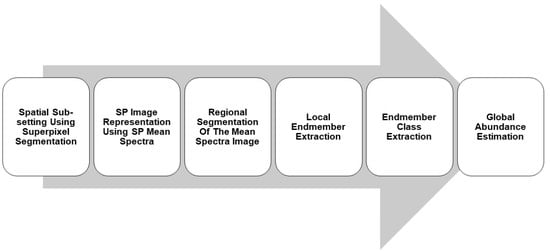
Figure 9.
Proposed unsupervised superpixel-based hyperspectral unmixing with regional segmentation.

Figure 10.
Illustration of quadtree image representation.

Figure 11.
HYDICE Urban Image: (a) true-color composite; (b) reference data classification map [42]; (c) endmembers.
Figure 11.
HYDICE Urban Image: (a) true-color composite; (b) reference data classification map [42]; (c) endmembers.

Figure 12.
ROSIS Pavia University (a) true-color composite; (b) reference class map; (c) endmembers.
Figure 12.
ROSIS Pavia University (a) true-color composite; (b) reference class map; (c) endmembers.

Figure 13.
SLIC representation of the HYDICE Urban scene: (a) SLIC over-segmentation; (b) SP representation, each pixel replace by the mean; (c) partitioning of the SP representation using quadtree (EMs = Endmembers per leave).
Figure 13.
SLIC representation of the HYDICE Urban scene: (a) SLIC over-segmentation; (b) SP representation, each pixel replace by the mean; (c) partitioning of the SP representation using quadtree (EMs = Endmembers per leave).

Figure 14.
Endmembers for each leaf tile in the Urban quadtree.

Figure 15.
Spectral signatures associated with the Urban information classes.

Figure 16.
Urban information classes’ abundance maps.

Figure 17.
Comparison between abundance maps for information classes extracted using the proposed method and reference data. The top row shows the results of the proposed method. The second row shows the reference data. The third row shows absolute errors images. The bottom row shows the histograms for the error images.

Figure 18.
Comparison of the information classes spectral endmembers extracted with the proposed algorithm and reference endmember spectral signatures. Top row: the results of the proposed approach; Second row: reference data.
Figure 18.
Comparison of the information classes spectral endmembers extracted with the proposed algorithm and reference endmember spectral signatures. Top row: the results of the proposed approach; Second row: reference data.

Figure 19.
Urban Image: (a) classification map derived from the abundances using winner takes it all and 50%threshold; (b) classification map after median filtering; (c) reference data classification map [42].
Figure 19.
Urban Image: (a) classification map derived from the abundances using winner takes it all and 50%threshold; (b) classification map after median filtering; (c) reference data classification map [42].

Figure 20.
SLIC superpixel representation of ROSIS Pavia image: (a) SLIC segmentation; (b) true-color display of the SP means image; (c) Pavia SP means image partitioning using quadtree (EMs = Endmembers per leave).
Figure 20.
SLIC superpixel representation of ROSIS Pavia image: (a) SLIC segmentation; (b) true-color display of the SP means image; (c) Pavia SP means image partitioning using quadtree (EMs = Endmembers per leave).

Figure 21.
Spectral endmembers for each leaf tile for the Pavia image.

Figure 22.
Spectral similarities in Pavia image: (a) spectral signatures highlighting similarities; (b) spatial location of spectrally similar information classes.
Figure 22.
Spectral similarities in Pavia image: (a) spectral signatures highlighting similarities; (b) spatial location of spectrally similar information classes.

Figure 23.
Spectral endmembers for each Pavia information class.

Figure 24.
Abundances for Pavia information classes.

Figure 25.
Comparison of Asphalt and Bitumen abundance map and binary reference map for Pavia.

Figure 26.
Comparison of Meadows and Bare Soil abundance and binary reference map for Pavia.

Figure 27.
Comparison between extracted abundance maps and binary class maps from reference data. The top row shows the abundancemaps and the bottomrow the binary classmaps fromthe reference data.
Figure 27.
Comparison between extracted abundance maps and binary class maps from reference data. The top row shows the abundancemaps and the bottomrow the binary classmaps fromthe reference data.

Figure 28.
Classification maps for Pavia: (a) classification map generated using winner takes it all with 50% threshold; (b) median filtered classification map; (c) classification map in (b) after masking non-assigned or background pixels in the reference data; (d) modified reference classification map.

Figure 29.
Comparison of abundance maps by different approaches with the proposed method and reference data.
Figure 29.
Comparison of abundance maps by different approaches with the proposed method and reference data.

Figure 30.
Comparison of extracted endmembers by different approaches with the proposed method and reference data.
Figure 30.
Comparison of extracted endmembers by different approaches with the proposed method and reference data.

Figure 31.
(a) quadtree image segmentation of the Urban scene; (b) number of endmembers per tile (total = 114).
Figure 31.
(a) quadtree image segmentation of the Urban scene; (b) number of endmembers per tile (total = 114).

Figure 32.
Comparison of extracted classification maps by different approaches with the proposed approach.
Figure 32.
Comparison of extracted classification maps by different approaches with the proposed approach.


Table 1.
Agreement matrix between reference and generated classification maps for Urban.
| Reference Data | ||||||||
|---|---|---|---|---|---|---|---|---|
| Road | Grass | Trees | Roof | Dirt | Totals | User’s Agreement (%) | ||
| Class Map | Road | 13,775 | 296 | 368 | 96 | 238 | 14,773 | 93.24 |
| Grass | 44 | 29,443 | 1162 | 34 | 223 | 30,906 | 95.27 | |
| Trees | 59 | 2633 | 20,068 | 188 | 31 | 22,979 | 87.33 | |
| Roof | 1569 | 400 | 2108 | 6106 | 871 | 11,054 | 55.24 | |
| Dirt | 717 | 1542 | 736 | 281 | 5543 | 8819 | 62.85 | |
| Un-Assigned | 1301 | 2197 | 1647 | 222 | 347 | 5714 | ||
| Totals | 17,465 | 36,511 | 26,089 | 6927 | 7253 | 94,245 | ||
| Producer’s agreement (%) | 78.87 | 80.64 | 76.92 | 88.15 | 76.42 | Overall agreement = 79.51% | ||
| Harmonic Mean (%) | 85.46 | 87.35 | 81.80 | 67.92 | 68.98 | Kappa Statistic = 73.06 % | ||
Table 2.
Agreement matrix between reference and filtered classification maps for Urban.
| Reference Data | ||||||||
|---|---|---|---|---|---|---|---|---|
| Road | Grass | Trees | Roof | Dirt | Totals | User’s Agreement (%) | ||
| Class Map | Road | 15,369 | 1187 | 758 | 88 | 345 | 17747 | 86.6 |
| Grass | 248 | 32,484 | 458 | 20 | 156 | 33,366 | 97.36 | |
| Trees | 442 | 1968 | 23,678 | 362 | 145 | 26,595 | 89.03 | |
| Roof | 1055 | 257 | 1082 | 6387 | 1086 | 9867 | 64.73 | |
| Dirt | 169 | 365 | 85 | 69 | 5510 | 6198 | 88.90 | |
| Un-Assigned | 182 | 250 | 28 | 1 | 11 | 472 | ||
| Totals | 17,465 | 36,511 | 26,089 | 6927 | 7253 | 94,245 | ||
| Producer’s agreement (%) | 88.00 | 88.97 | 90.76 | 92.20 | 75.97 | Overall agreement = 88.52% | ||
| Harmonic Mean (%) | 87.29 | 92.97 | 89.89 | 76.06 | 81.93 | Kappa Statistic = 84.43 % | ||
Table 3.
Agreement matrix between reference and generated classification maps for Pavia.
| Reference Data | |||||||||
|---|---|---|---|---|---|---|---|---|---|
| Asphalt and Bitumen | Meadows and Soil | Gravel and Brick | Trees | Metal Sheet | Shadow | Totals | User’s Agreement (%) | ||
| Class Map | Asphalt and Bitumen | 3933 | 190 | 497 | 2 | 6 | 112 | 4740 | 82.97 |
| Meadows and Soil | 28 | 19,012 | 16 | 925 | 2 | 0 | 19,983 | 95.14 | |
| Gravel and Brick | 282 | 536 | 4224 | 4 | 1 | 0 | 5047 | 83.69 | |
| Trees | 0 | 683 | 0 | 1874 | 0 | 0 | 2557 | 73.29 | |
| Metal Sheet | 1 | 0 | 0 | 0 | 1225 | 0 | 1226 | 99.84 | |
| Shadow | 24 | 4 | 3 | 2 | 2 | 433 | 468 | 92.52 | |
| Un-Assigned | 3658 | 2161 | 1046 | 194 | 77 | 560 | 7696 | ||
| Totals | 7926 | 22,586 | 5786 | 3001 | 1313 | 1105 | 41,717 | ||
| Producer’s agreement (%) | 49.62 | 84.18 | 73.00 | 62.45 | 93.30 | 39.19 | Overall agreement = 73.59% | ||
| Harmonic Mean (%) | 62.10 | 89.32 | 77.98 | 67.43 | 96.49 | 55.05 | Kappa Statistic = 62.10% | ||
Table 4.
Agreement matrix between reference and filtered classification maps for Pavia.
| Reference Data | |||||||||
|---|---|---|---|---|---|---|---|---|---|
| Asphalt and Bitumen | Meadows and Soil | Gravel and Brick | Trees | Metal Sheet | Shadow | Totals | User’s Agreement (%) | ||
| Class Map | Asphalt and Bitumen | 4168 | 327 | 768 | 42 | 20 | 208 | 5533 | 75.33 |
| Meadows and Soil | 0 | 21,355 | 134 | 1106 | 6 | 10 | 22,611 | 94.45 | |
| Gravel and Brick | 0 | 493 | 4538 | 10 | 10 | 1 | 5052 | 89.83 | |
| Trees | 0 | 208 | 0 | 1751 | 0 | 5 | 1964 | 89.15 | |
| Metal Sheet | 0 | 0 | 0 | 0 | 1259 | 4 | 1263 | 99.68 | |
| Shadow | 0 | 0 | 0 | 0 | 0 | 383 | 383 | 100 | |
| Un-Assigned | 3431 | 732 | 225 | 95 | 27 | 605 | 5115 | ||
| Totals | 7599 | 23,115 | 5665 | 3004 | 1322 | 1216 | 41,921 | ||
| Producer’s agreement (%) | 54.85 | 92.39 | 80.11 | 58.29 | 95.23 | 31.50 | Overall agreement = 79.80% | ||
| Harmonic Mean (%) | 63.48 | 93.40 | 84.69 | 70.49 | 97.41 | 47.90 | Kappa Statistic = 69.30% | ||
Table 5.
Agreement matrix between Full Global and reference map.
| Reference Data | ||||||||
|---|---|---|---|---|---|---|---|---|
| Road | Grass | Trees | Roof | Dirt | Totals | User’s Agreement (%) | ||
| Class Map | Road | 5501 | 187 | 134 | 79 | 63 | 5964 | 92.24 |
| Grass | 1020 | 35,009 | 3711 | 265 | 2346 | 42,351 | 82.66 | |
| Trees | 348 | 153 | 20,654 | 961 | 208 | 22,324 | 92.52 | |
| Roof | 790 | 71 | 160 | 4727 | 108 | 5856 | 80.72 | |
| Dirt | 1481 | 369 | 309 | 126 | 3328 | 5613 | 59.29 | |
| Un-Assigned | 8325 | 722 | 1121 | 769 | 1200 | 12,137 | ||
| Totals | 17,465 | 36,511 | 26,089 | 6927 | 7253 | 94,245 | ||
| Producer’s agreement (%) | 31.50 | 95.89 | 79.17 | 68.24 | 45.88 | Overall agreement = 73.45% | ||
| Harmonic Mean (%) | 46.96 | 88.79 | 85.32 | 73.96 | 51.73 | Kappa Statistic = 64.09% | ||
Table 6.
Agreement matrix between SP Global and reference map.
| Reference Data | ||||||||
|---|---|---|---|---|---|---|---|---|
| Road | Grass | Trees | Roof | Dirt | Totals | User’s Agreement (%) | ||
| Class Map | Road | 16,476 | 4280 | 2256 | 756 | 5993 | 29,761 | 55.36 |
| Grass | 70 | 28,905 | 592 | 132 | 84 | 29,783 | 97.05 | |
| Trees | 117 | 2399 | 22,656 | 841 | 185 | 26,198 | 86.48 | |
| Roof | 738 | 76 | 315 | 4748 | 66 | 5943 | 79.89 | |
| Dirt | 0 | 53 | 25 | 289 | 594 | 961 | 61.81 | |
| Un-Assigned | 64 | 798 | 245 | 161 | 331 | 1599 | ||
| Totals | 17,465 | 36,511 | 26,089 | 6927 | 7253 | 94,245 | ||
| Producer’s agreement (%) | 94.34 | 79.17 | 86.84 | 68.54 | 8.19 | Overall agreement = 77.86% | ||
| Harmonic Mean (%) | 79.78 | 87.20 | 86.66 | 73.78 | 14.46 | Kappa Statistic = 69.95% | ||
Table 7.
Agreement matrix between Full+QT and reference map.
| Reference Data | ||||||||
|---|---|---|---|---|---|---|---|---|
| Road | Grass | Trees | Roof | Dirt | Totals | User’s Agreement (%) | ||
| Class Map | Road | 16,080 | 1973 | 1215 | 282 | 444 | 19,994 | 80.42 |
| Grass | 51 | 31,226 | 1055 | 78 | 320 | 32,730 | 95.40 | |
| Trees | 136 | 1190 | 22,117 | 460 | 221 | 24,124 | 91.68 | |
| Roof | 793 | 125 | 888 | 6008 | 1157 | 8971 | 66.97 | |
| Dirt | 54 | 963 | 35 | 9 | 4752 | 5813 | 81.75 | |
| Un-Assigned | 351 | 1034 | 779 | 90 | 359 | 2613 | ||
| Totals | 17,465 | 36,511 | 26,089 | 6927 | 7253 | 94,245 | ||
| Producer’s agreement (%) | 92.07 | 85.52 | 84.78 | 86.73 | 65.52 | Overall agreement = 85.08% | ||
| Harmonic Mean (%) | 85.85 | 90.20 | 88.09 | 75.58 | 72.74 | Kappa Statistic = 79.93% | ||
Table 8.
Comparing harmonic means, Cohen’s kappa and overall agreement (OA) for the four methods.
| Class Harmonic Means | |||||||
|---|---|---|---|---|---|---|---|
| Road | Grass | Trees | Roof | Dirt | Kappa (%) | OA (%) | |
| Proposed: SP + QT | 87.29 | 92.97 | 89.89 | 76.06 | 81.93 | 84.43 | 88.52 |
| Full + QT | 85.85 | 90.20 | 88.09 | 75.58 | 72.74 | 79.93 | 85.08 |
| SP Global | 79.78 | 87.20 | 86.66 | 73.78 | 14.46 | 69.95 | 77.86 |
| Full Global | 46.96 | 88.79 | 85.32 | 73.96 | 51.73 | 64.09 | 73.45 |
© 2019 by the authors. Licensee MDPI, Basel, Switzerland. This article is an open access article distributed under the terms and conditions of the Creative Commons Attribution (CC BY) license (http://creativecommons.org/licenses/by/4.0/).
Share and Cite
MDPI and ACS Style
Alkhatib, M.Q.; Velez-Reyes, M. Improved Spatial-Spectral Superpixel Hyperspectral Unmixing. Remote Sens. 2019, 11, 2374. https://doi.org/10.3390/rs11202374
AMA Style
Alkhatib MQ, Velez-Reyes M. Improved Spatial-Spectral Superpixel Hyperspectral Unmixing. Remote Sensing. 2019; 11(20):2374. https://doi.org/10.3390/rs11202374
Chicago/Turabian StyleAlkhatib, Mohammed Q., and Miguel Velez-Reyes. 2019. "Improved Spatial-Spectral Superpixel Hyperspectral Unmixing" Remote Sensing 11, no. 20: 2374. https://doi.org/10.3390/rs11202374
Note that from the first issue of 2016, this journal uses article numbers instead of page numbers. See further details here.