A Structural Classification of Australian Vegetation Using ICESat/GLAS, ALOS PALSAR, and Landsat Sensor Data

Abstract

Australia has historically used structural descriptors of height and cover to characterize, differentiate, and map the distribution of woody vegetation across the continent but no national satellite-based structural classification has been available. In this study, we present a new 30-m spatial resolution reference map of Australian forest and woodland structure (height and cover), with this generated by integrating Landsat Thematic Mapper (TM) and Enhanced TM, Advanced Land Observing Satellite (ALOS) Phased Arrayed L-band Synthetic Aperture Radar (PALSAR) and Ice, Cloud, and land Elevation (ICESat),and Geoscience Laser Altimeter System (GLAS) data. ALOS PALSAR and Landsat-derived Foliage Projective Cover (FPC) were used to segment and classify the Australian landscape. Then, from intersecting ICESat waveform data, vertical foliage profiles and height metrics (e.g., 95% percentile height, mean height and the height to maximum vegetation density) were extracted for each of the classes generated. Within each class, and for selected areas, the variability in ICESat profiles was found to be similar with differences between segments of the same class attributed largely to clearance or disturbance events. ICESat metrics and profiles were then assigned to all remaining segments across Australia with the same class allocation. Validation against airborne LiDAR for a range of forest structural types indicated a high degree of correspondence in estimated height measures. On this basis, a map of vegetation height was generated at a national level and was combined with estimates of cover to produce a revised structural classification based on the scheme of the Australian National Vegetation Information System (NVIS). The benefits of integrating the three datasets for segmenting and classifying the landscape and retrieving biophysical attributes was highlighted with this leading the way for future mapping using ALOS-2 PALSAR-2, Landsat/Sentinel-2, Global Ecosystem Dynamics Investigation (GEDI), and ICESat-2 LiDAR data. The ability to map across large areas provides considerable benefits for quantifying carbon dynamics and informing on biodiversity metrics.

1. Introduction

A large number of studies have focused on quantifying the height of woody vegetation at regional to global scales from remote sensing data, with these based primarily on radar interferometry (e.g., the Shuttle Radar Topographic Mission (SRTM) from 2000) and Tandem-X (from 2010 onwards) or spaceborne LiDAR (namely, the ICESat/GLAS from 2003–2008). In the case of radar interferometry, continuous (wall-to-wall) height mapping has been achieved. As examples, [1,2] used SRTM data to generate height maps for mangroves in Africa and forests across the conterminous United States, respectively. However, with the ICESat/GLAS data, the landscape is only sampled and hence a mechanism for extrapolating the retrieved height or other measures across the remaining landscape is necessary [3,4,5].

Several early approaches to extrapolation have been developed using airborne LiDAR data. For example, [3,4,6] related ground-based or airborne LiDAR-derived estimates of biomass or volume to intersecting ICESat/GLAS metrics thereby allowing these measures to be extrapolated across the landscape, albeit as samples. Wall-to-wall mapping of vegetation height was achieved by [7], who used the eCognition software to generate a nested segmentation of the landscape based on the SRTM National Elevation Dataset (NED)-derived slope, the SRTM-NED difference and the National Land Cover Database (NLCD) of canopy density. They then extrapolated associated airborne Laser Vegetation Imaging Sensor (LVIS) metrics across segments based on an inverse weighted distance. Ørka et al. [8] also generated a wall-to-wall coverage of canopy cover by extrapolating estimates from airborne LiDAR data using a random forest, non-parametric classification of Landsat-derived Normalized Difference Vegetation Index (NDVI) data, Tasseled Cap transformed brightness and wetness, and elevation and slope data.

Coarse resolution (~0.5° × 0.5°) gridded global vegetation height map, such as Los et al. [9], can be derived directly from aggregated ICESat/GLAS footprints with filters (e.g., slope, elevation, area under first Gaussian) applied to remove anomalous data. However, previous work to extrapolate ICESat-derived height metrics to form continuous height surfaces at moderate spatial resolution has relied on the use of other spatially continuous moderate resolution remote sensing datasets. For example, Lefsky et al. [10] associated ICESat footprints with forest area segments (based on spectral and textural heterogeneity properties) generated from MODIS data. For those segments without GLAS data, canopy height prediction equations were developed for each of six geographic regions using Cubist (a rule-based modeling approach) to extrapolate using MODIS attributes such as forest cover fraction, brightness, principal component bands, greenness indices, and cover and biome type. In a similar fashion, Simard et al. [11] employed a Random Forest regression tree method to model RH100 values (the distance between signal beginning and the location of the lidar ground peak) based on global climate and vegetation variables (precipitation, precipitation seasonality, annual mean temperature, temperature seasonality, elevation, percent forest cover, and protection status) for areas not covered by GLAS waveforms [9]. Chi et al. [12] extended this approach by adding an improved slope correction method. However, these continental scale methods have all relied on optical data, predominantly from the MODIS sensor, thus limiting the spatial resolution of the final map.

This study recognized the benefits of low frequency Synthetic Aperture Radar (SAR) for providing information on the woody components of vegetation which was complementary to the use of optical data. Hence the aim was to investigate the use of ALOS PALSAR L-band HH and HV data and Landsat-derived Foliage Projective Cover (FPC) [13] for extrapolating ICESat/GLAS waveforms and associated vegetation height and cover metrics across Australia with a view to generating a new national structural classification. The objectives were to (a) use the ALOS PALSAR and Landsat sensor data to segment the Australian landscape into structurally homogeneous units, given their sensitivity to the woody and foliage components of vegetation respectively, (b) cluster these segments using these same data to establish those that were most similar, (c) associate each resulting class with height and cover metrics derived from ICESat/GLAS waveform data thereby allowing national extrapolation, and (d) evaluate the accuracy of metric retrievals through reference to airborne LiDAR data to give confidence in the resulting product.

2. The Australian Landscape and Vegetation

Australia has a diverse landscape, with this conveyed by the division into 89 largely distinct bioregions defined through the Interim Biogeographic Regionalization for Australia (IBRA) on the basis of similarities in climate, geology, landform, native vegetation and dominant plant species. These regions are further divided into 419 subregions [14]. Nearly 91% of Australia (or nearly seven million km²) is occupied by vegetation (Figure 1), with forest occurring over 21.3% of the area. Over 23% of the country is dominated by hummock grasslands, with these largely occurring in West Australia, South Australia, and the Northern Territory. Forests are associated with vegetation dominated by trees having usually a single stem and a mature or potentially mature stand height exceeding 2 m and with the existing or potential crown cover of overstorey strata ≥20%. The classification of Specht [15] relevant to forests is based on the three structural attributes of height and foliage projective cover (FPC) of the tallest plant layer as well as dominant functional type or plant form (trees or shrubs;

Table 1. Overview of structural formations used in this paper adapted from [15] and [18] and the National Vegetation Inventory System (NVIS) structural formation terminology [17].

Lifeform and Height of the Tallest Stratum	Foliage Projective Cover (FPC) or Crown Cover (CC) of the Tallest Plant Layer
	Dense 70–100% FPC >80% CC	Mid-dense 30–70% FPC 50–80% CC	Sparse 10–30% FPC 20–50% CC	Very Sparse/Isolated <10% FPC 0.25–20% CC
Trees > 30 m	tall closed forest	tall open forest	tall woodland	tall open woodland
Trees 10–30 m	closed forest	open forest	woodland	open woodland
Trees 5–10 m	low closed forest	low open forest	low woodland	low open woodland
Shrubs 2–8 m	closed scrub	open scrub	tall shrubland	tall open shrubland
Shrubs 0–2 m	closed heath	open heath	low shrubland	low open shrubland

). Within the classification system of Carnahan [16], additional floristic information is included (e.g., whether the dominant genus present in the upper stratum (primarily) is Eucalyptus, Acacia, Banksia, Casuarina, Hakea, or Melaleuca). Australia’s National Vegetation Information System (NVIS; [17]), which standardized vegetation information across the States and Territories, also recognized height and cover as important descriptors and used these in conjunction with floristic information and terminologies of Specht [15], Specht and Specht [18], and also Walker and Hopkins [19] to classify 23 Major Vegetation Groups (Figure 1). Trees and palms are associated with closed and open forest, woodland and open woodlands and isolated clumps of trees. Shrublands are typically < 2 m in height but mallee (which occurs in the more semi-arid area) supports shrubs and trees that are up to 8 and 10 m, respectively. The NVIS utilized existing and many finer detailed classifications undertaken by the Australian States and Territories to generate the nationally consistent classification. Within the mapping, and at the time of generation, noticeable discontinuities were observed between datasets and there were gaps in scale, current, and detail.

3. Methods

3.1. Remote Sensing Data

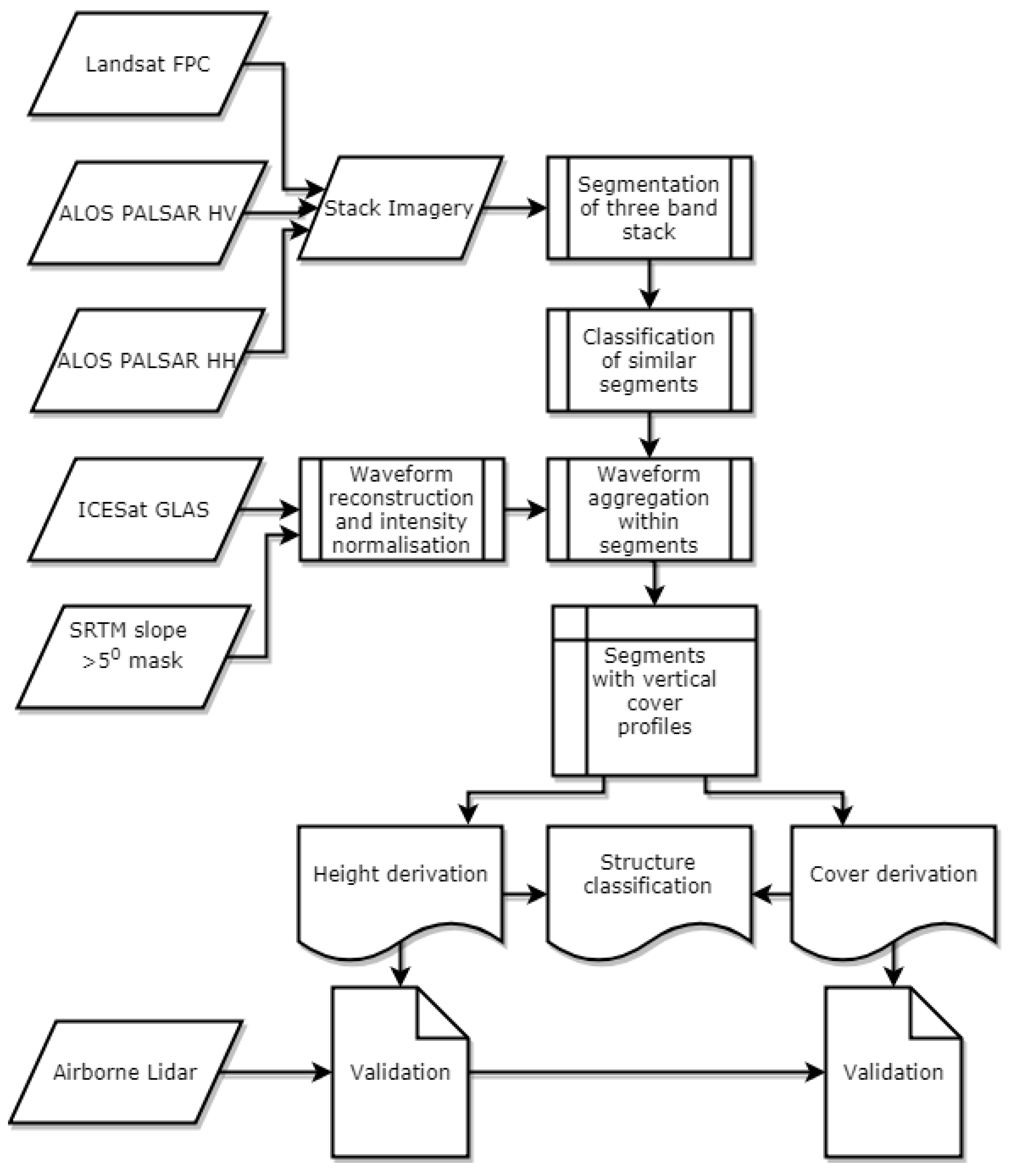
ALOS PALSAR L-band Fine Beam Dual (HH and HV) mosaic product data for 2010 were provided at 25 m spatial resolution through the Japanese Space Exploration Agency (JAXA) Kyoto and Carbon (K&C) Initiative. These data had been orthorectified, topographically corrected and calibrated using procedures outlined by Shimada et al. [20]. The orthorectification utilized a DEM simulated from SRTM data and ALOS PALSAR strips acquired during periods of relatively low surface moisture were used to generate the mosaic as proposed by Lucas et al. [21]. Correction procedures were also applied to remove across and between track variations in backscatter associated primarily with varying moisture conditions and incidence angles. Using multi-year (1987 to 2010) dry season (May to October inclusive) Landsat sensor data, a 30 m spatial resolution FPC product for 2010 was generated, from which the seasonal signal associated with herbaceous vegetation had been removed [13]. These data were combined into a 30 m spatial resolution image stack by cubic convolution resampling of the ALOS PALSAR mosaics onto the Landsat FPC product pixel grid. ICESat/GLAS L2 (Release 33) Global Land Surface Altimetry (GLA14) data acquired between 2003 and 2009 were obtained from the National Snow and Ice Data Centre (NSIDC). These data were acquired over variable footprint sizes and intensities but footprints were distributed unevenly across the landscape. An overview of the available datasets is provided in Figure 2, which shows a color composite of the Landsat FPC, ALOS PALSAR L-band HH and HV data (in RGB) with the ICESat tracks across Australia.

3.2. Analysis

The approach to extrapolation of the ICESat height metrics (Figure 3) focused first on segmentation (based on k-means clustering and iterative elimination; [22]) of the ALOS PALSAR HH and HV and Landsat FPC data and subsequent classification of the resulting segments. A k-means clustering of the mean HH and HV and Landsat FPC values within each segment was then undertaken to provide clusters of segments with similar backscatter and cover statistics. The k-means method was used as it represented the simplest reproducible and scalable method that was applicable to the classification task and other approaches (e.g., agglomerative hierarchical clustering, mean shift, and variational Bayesian Gaussian mixture models) were too slow and memory intensive for our dataset size. ICESat-derived structural metrics were then assigned to all non-intersecting segments based on their class allocation. Finally, validation of the height metrics was undertaken through reference to independently acquired airborne LiDAR data across and range of forest structural types. The following sections outline these steps in more detail.

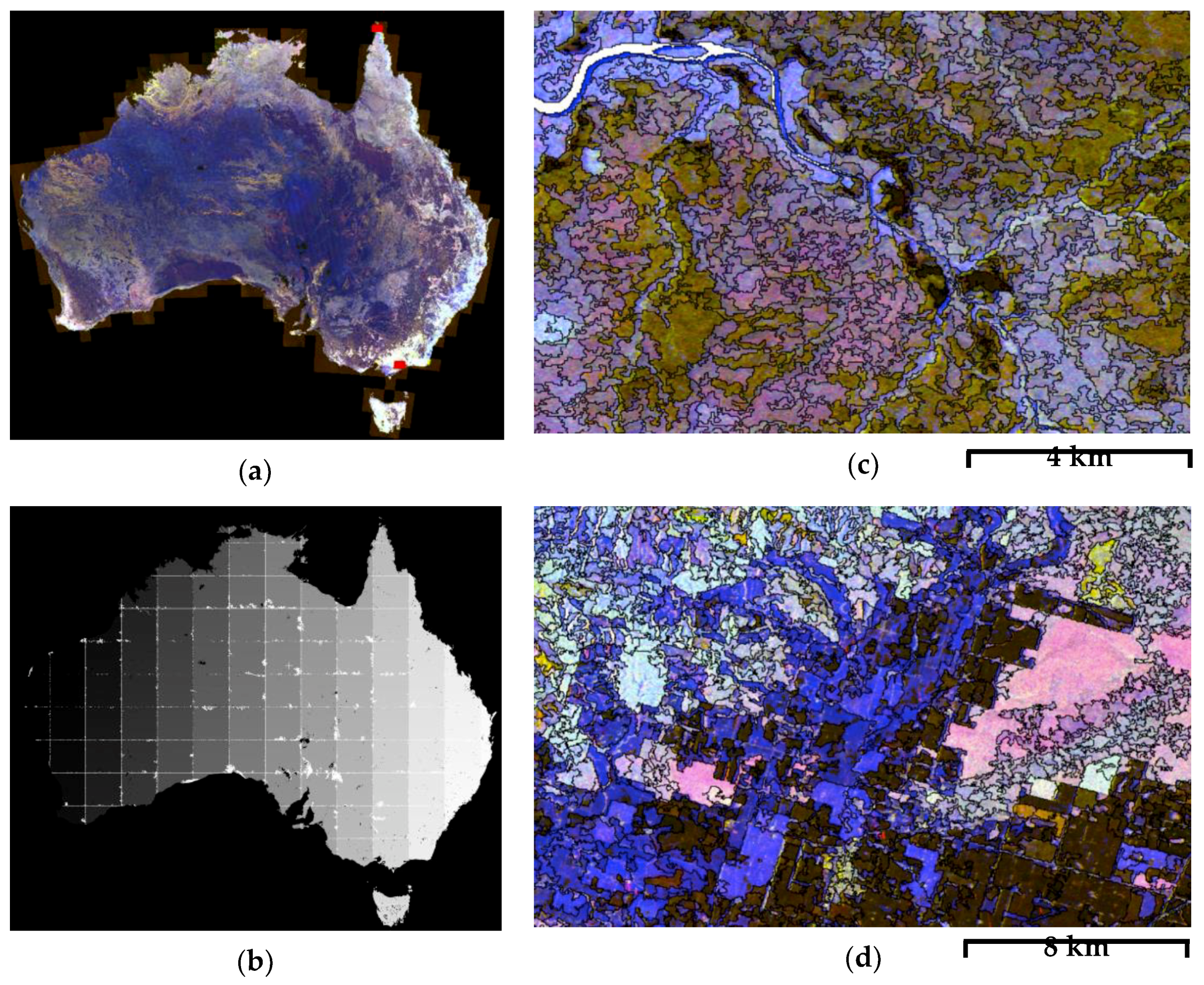
3.2.1. Segmentation of ALOS PALSAR and Landsat Data

To define homogeneous regions for classification, the segmentation approach of Shephard et al. [23] was applied to the ALOS PALSAR L-band HH and HV and Landsat-derived FPC in combination. This method was chosen as it provides a highly scalable open source framework enabling continental scale segmentation and also support for a minimum mapping unit through an iterative elimination process. Initially, the input data were normalized based on a two-standard-deviation normalization to ensure that all bands were equally weighted. A k-means clustering was used subsequently to identify the mean spectra within the images where the number of clusters, k, was user defined (in this case, 60). The image pixels were then subsequently labeled according to the k-means cluster numbers before being merged into discrete regions. Regions under a minimum user defined object size (a threshold of 100 pixels was used in this case) were then removed iteratively, being merged into the neighboring clump with the shortest Euclidean distance defined using the normalized L-HH, L-HV and FPC values. The elimination started with features 1 pixel in size and incrementally eliminated features of larger sizes in 1-pixel steps (i.e., 1 to n pixels). When all neighbors were of a size equivalent to the current feature, no further elimination took place and the feature was only then eliminated in a subsequent iteration. Following elimination, the features were relabeled to ensure that they were numbered sequentially. Examples of the segmentation are shown in Figure 4.

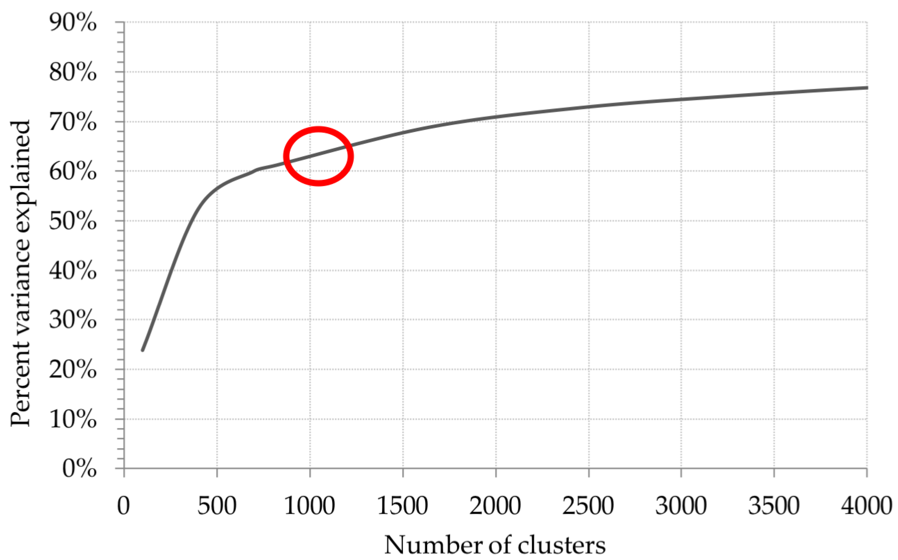
3.2.2. Clustering of Segments

Collectively and broadly, the ALOS PALSAR HH and HV data and the Landsat FPC broadly provide a spatial indication of the relative amounts of trunk, large branch, and foliage within the forest volume [24]. Hence, objects generated through segmentation of these data should represent, in principle, vegetation of similar structure. However, due to landscape and landform variability and fragmentation, segments associated with forests of similar structural form may be separated spatially. Therefore, the k-means clustering algorithm (from scikit-learn; [25]) was used to classify segments into clusters with similar values of L-band HH and HV and Landsat FPC. For this, the elbow method was used to estimate the optimal number of clusters. It is noted that the ‘elbow’ cannot always be unambiguously identified [26] so a certain amount of manual interpretation is required to achieve the best results. The percentage of variance explained as a function of the number of clusters was calculated by generated statistics for cluster numbers between 100 and 8000. In this application, it was important to cumulate as many ICESat returns in each class as possible, whilst still retaining a sufficient number of clusters to capture the variability in Australian vegetation communities. Figure 5 shows that the elbow can be found at around 500 clusters. In this work, 1000 classes were selected after visual inspection of the 500-cluster classification showed some important smaller landscape features areas (such as patches of regrowth and plantation) were being linked to classes in quite different environments.

3.2.3. ICESat/GLAS Processing

The ICESat orbital strip data, which were provided in binary format, were decoded using a data dictionary to extract the location, elevation, time, pulse eccentricity, intensity and size as well as the Gaussian decomposition parameters of the retrieved waveform. The sequence of processing is outlined below.

In determining the profile relating to the vertical distribution of plant material, the ground return was assumed to be the Gaussian with the lowest elevation, thereby allowing separation from the vegetation return. Whilst in the majority of cases, correct retrieval occurs, multiple ground pulses may occur in areas of complex terrain or no ground pulse will be received when the canopy cover is extremely high. Across much of Australia, the landscape is relatively level (with slopes typically < 5°) although there are significant areas of relief (e.g., on the east coast), including within gorges and river channels.

Following identification of the ground return, each individual vegetation ICESat/GLAS pulse was reconstructed from the Gaussian decomposition using

$$I_v\left(z\right)={\displaystyle \sum _{m=1}^N{A}_m{e}^{-\frac{z-{\mu }_m}{2{\sigma }_m^2}}},$$

(1)

where I_v(z) is the pulse intensity vegetation as a function of distance z, N is the number of peaks found in the waveform, and A_m, σ_m and u_m represent the amplitude, centroid and standard deviation of the m^th peak. The ground pulse was reconstructed using

$$I_g\left(z\right)=A_g{e}^{-\frac{z-{\mu }_g}{2{\sigma }_g^2}},$$

(2)

where I_g(z) is the pulse intensity of the ground as a function distance z, and A_g, σ_g, and u_g are the amplitude, centroid, and standard deviation of the identified ground peak. Both the ground and vegetation waveforms were then normalized by the transmitted pulse intensity to account for the different laser systems using

$$\omega \left(z\right)=\frac{I\left(z\right)}{I_T},$$

(3)

where $\omega \left(z\right)$ is the normalized waveform and $I_T$ is the reported transmitted pulse intensity derived from the GLA14 data file. All the normalized ground and vegetation waveforms for each cluster were then summed to produce the final representative waveform.

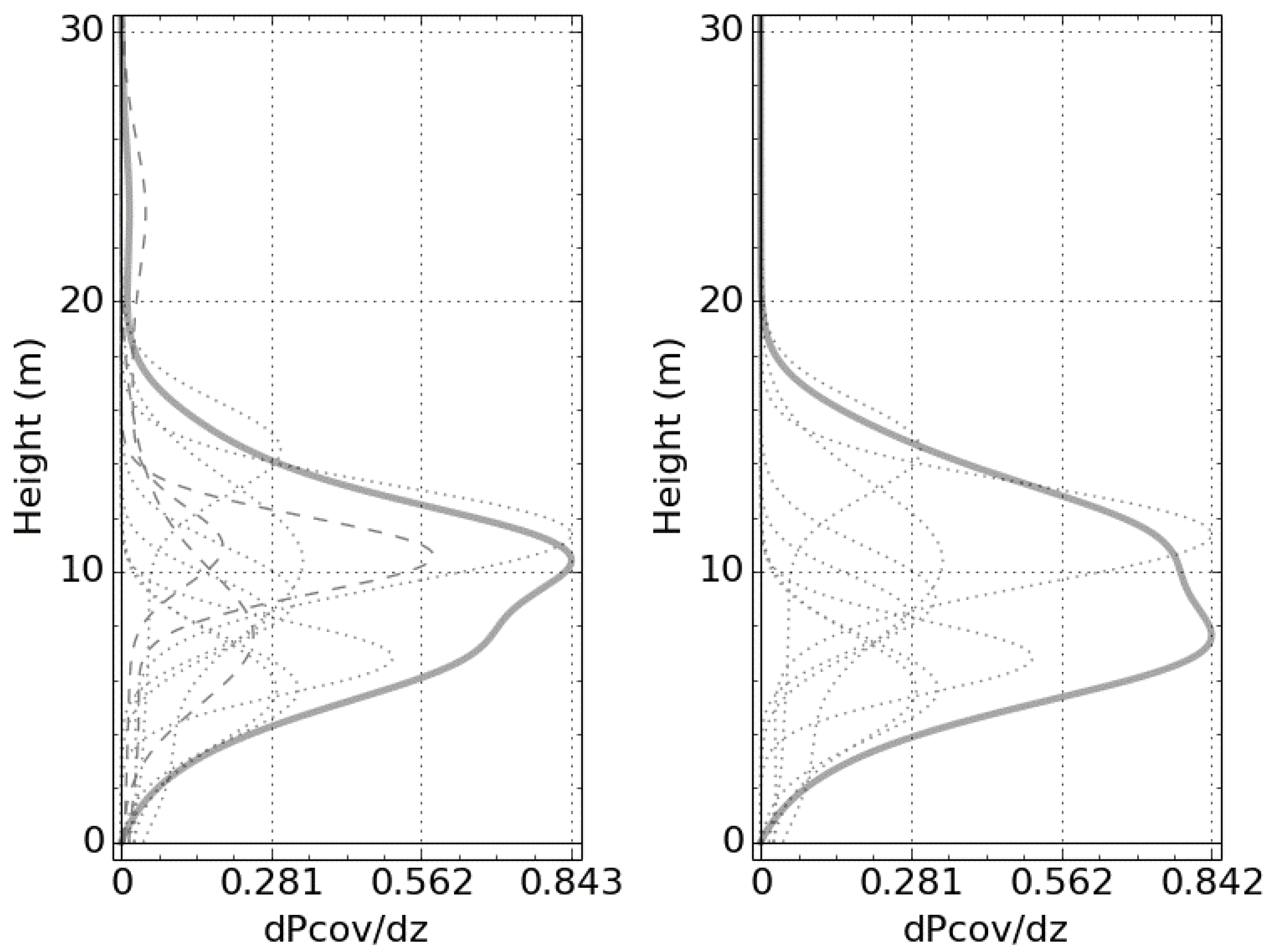
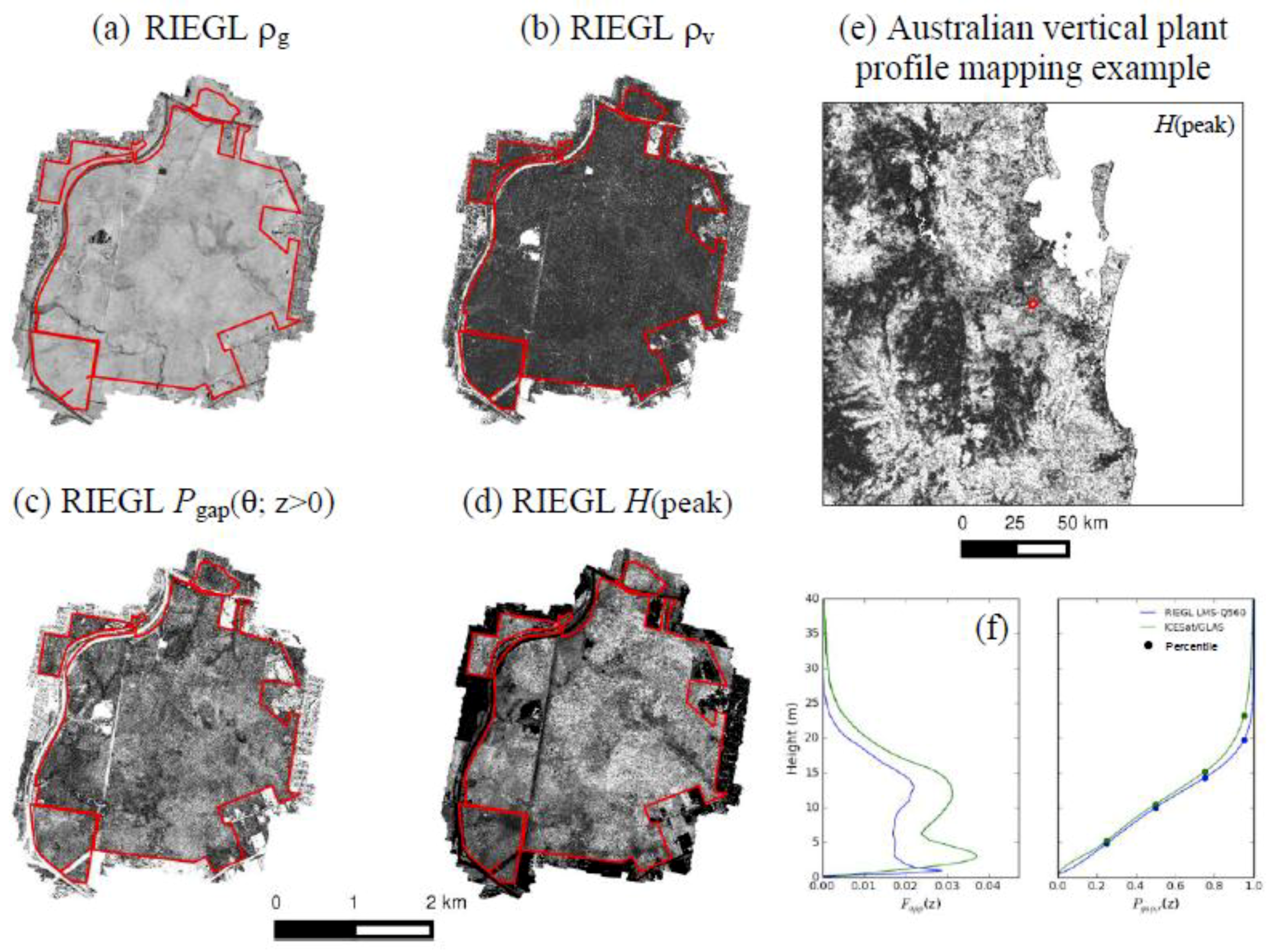
3.3. Vertical Cover Profile Derivation

From the cluster mean vegetation waveform, the cumulative vertical cover ($1-P_{gap}\left(z\right)$) profiles were computed using

$$C\left(z\right)=\frac{{\rho }_g^z{\omega }_v\left(z\right)}{{\rho }_v{\displaystyle \sum }{\omega }_g\left(z\right)+{\rho }_g{\displaystyle \sum }{\omega }_v\left(z\right)},$$

(4)

where ${\rho }_g^z{\omega }_v(z)$ represents the cumulative sum of the vegetation waveform and ${\rho }_v$ and ${\rho }_g$ are the apparent reflectances of the vegetation and ground at the LiDAR wavelength (1064 nm). Cluster-based ${\rho }_g$ and ${\rho }_v$ estimates were obtained from the reflectances reported in the GLA14 data file. For this, the vector of unknown component reflectances, $\rho =\frac{{\rho }_v}{{\rho }_g}$ was solved by using the method of least squares on $A\rho =r$, where A is the 2 × n matrix of the integrated pulse areas for the n vegetation and ground return pulses respectively and r is the vector of n GLAS reflectance estimates. The nominal vegetation canopy cover estimate C_t was then derived from the cumulative vertical cover profile using

$$C_t=\max \left(C\left(z\right)\right),$$

(5)

The waveform, cumulative vertical cover profiles and the canopy cover were used to calculate four canopy height metrics, with these being the mode (height to maximum vegetation density), average (with values above representing more than 50% of green material) and the 75th and the 95th percentile. These represented the height of peak cover and the vertical position where the cumulative foliage profile equals 50, 75, and 95% of the nominal cover estimate respectively. Cover was also derived as an integral of the waveform and as a function of amplitude. The roughness of the ground layers was described using the standard deviation of the ground surface.

The height and cover metrics were calculated for slopes < 5°. When this threshold is applied, the canopy of the tree on the lower slope is still above the ground on the upper slope. In some studies (e.g., [27]), a correction for slope was applied using existing elevation layers including the SRTM [27] and the US National Elevation Dataset (NED) [28]. In others (e.g., [29]), a minimum slope of 10° was used; however, a more stringent threshold was applied in this case given that the forests considered are lower in stature compared to other studies (e.g. [29]). The impact of slope is illustrated in Figure 6, which highlights the variability of waveforms in steeper terrain.

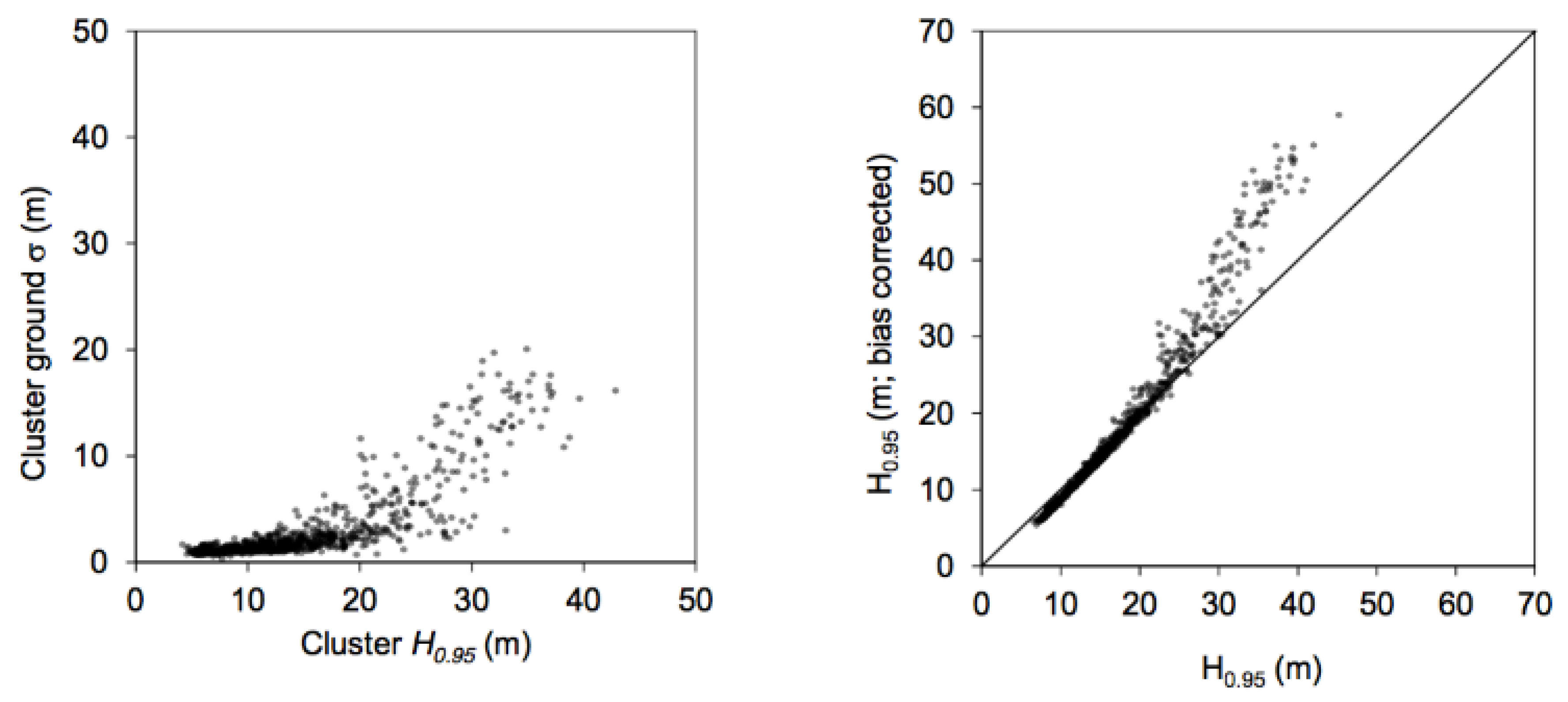
3.4. Height Metric Bias Correction

One issue with estimates using ICESat in particularly dense forests is that the height is typically underestimated, with the reason being minimal penetration to the ground surface. For this reason, the fitted Gaussian return can often merge the understorey and ground returns, particularly when the ground surface is rough. However, a monotonic relationship is observed between the ground surface standard deviation and the 95th percentile height for any given cluster (Figure 7), indicating a systematic bias in percentile heights. Since high slope areas are filtered out of the analysis, large ground surface standard deviations are attributable to local roughness or a merging of the ground and understorey layers. This bias in percentile height ($H_p$) can be removed through an empirical height correction by

$$H_{p,c}=\left(H_p-\frac{90\sin \left(s\right)}{2}\right)+\left(\sigma -{\sigma }_0\right)$$

(6)

where $\sigma$ is the mean cluster Gaussian width of the ground return, ${\sigma }_0$ is the mean cluster Gaussian width of a flat surface ground return derived from ICESat tracks over Lake Eyre, Australia. The slope, s, is the mean SRTM derived slope, and $H_{p,c}$ is the corrected percentile height.

3.5. Imputation of Metrics

Within each of the classified segments where ICESat waveforms intersected, a description of the forest structure was generated, with this including standard statistics (e.g., mean, standard deviation) for height and cover metrics. Pulses were omitted if the slope was > 50, with this being lower than the 10° threshold suggested by Rosette et al. [30]. A minimum of seven returns was needed to provide a description, with this minimum determined a priori based on progressive omission of profiles from segments with larger numbers (e.g., 50 waveforms). Consideration was also given to the location of the points and the laser used, as different laser intensities and signal to noise ratios (SNR) occur; hence the pulse were normalized. Variations in the pulse size were also considered.

3.6. Validation

Validation of height metrics derived from the ICESat/GLAS foliage profiles was achieved by comparison with equivalent airborne waveform LiDAR derived foliage profiles generated at a number of existing Terrestrial Ecosystem Research Network (TERN) Landscape Assessment sites across Australia (

Table 2. Names, location, and description of the Terrestrial Ecosystem Research Network (TERN) Auscover sites across Australia used for validation of the ICESat/GLAS height metrics.

Site Name	Longitude	Latitude	Environment
Chowilla (Calperum Mallee)	140.59	−34.00	Semi-arid mallee ecosystem in dune and swale system covered with an open mallee woodland upper story with a chenopod and native grass understory.
Watts Creek	145.68	−37.69	Open forest with a eucalypt overstorey greater than 40 m in height consisting mainly of mountain ash.
Rushworth Forest	144.96	−36.76	Open forest of red iron bark, red stringybark, red box, long leaf box, and grey box.
Zig Zag Creek	148.28	−37.48	Dominated by shrubby dry forest and damp forest on the upland slopes, wet forest ecosystems which are restricted to the higher altitudes and grassy woodlands, grassy dry forest and valley grassy forest ecosystems are associated with major river valleys.
Credo (Great Western Woodlands)	120.64	−30.19	Open woodland inter-dispersed with open, treeless areas. Main vegetation species are Salmon Gums up to 20 m and Gimlet between 5–10 m, both with little understory. Salt bush and similar shrubs are also prevalent.
South East Queensland	153.09	−27.63	Karawatha Forest: bushland with tall eucalypt species and patches of heatlands and Melaleuca swamps.
Litchfield	130.79	−13.18	Savanna, eucalypt open forests, dominated by Eucalyptus miniata and Eucalyptus tetrodonta.
Alice Mulga	133.25	−22.28	Mulga (Acacia aneura) canopy, which is 6.5 m tall on average.
Warra	146.66	−43.09	Homogenous tall, wet Eucalyptus obliqua forest with wet sclerophyll/rainforest understorey.

). The TERN sites were selected to represent dominant and/or conservation significant biomes in Australia and be suitable for scaling up from field and airborne measurements to continental scale map products for calibration and validation purposes [31]. Each site was approximately 5 × 5 km and was acquired by Airborne Research Australia (ARA) using a RIEGL LMS-Q560 waveform recording airborne laser scanner. The wavelength of the instrument laser was 1550 nm, the nominal flying height was 300m, the instrument laser pulse repetition rate was 240 kHz, and wall-to-wall coverage of each site was acquired with 50% swath overlap between flightlines.

Due to the availability of airborne waveform LiDAR, vertical cover profiles were retrieved directly using the approach of Armston et al. [32], which previously developed and validated a simple method for the retrieval of P_gap(θ,z) using Gaussian reconstructed waveforms calibrated to apparent reflectance. In this study, we extended the approach to map P_gap(θ) at high spatial resolution across large areas. If the method of [32] is to be widely useful, a practical mapping approach applicable at the sampling resolution of different waveform instruments was required. According to Equation. 16 from Armston et al. [32], we can estimate P_gap (1-C) by calculating from the attenuated signal, which only requires a modeled estimate of the ground apparent reflectance (${\rho }_g$)

$$P_{gap}\left(\mathsf{\theta },\mathrm{z}\right)=1-\frac{R_v\left(z=z_i\right)}{R_v}\frac{1}{1+R_g\left({\rho }_g-R_g\right)}$$

(7)

High spatial resolution samples of ${\rho }_g$ are available from these small footprint data as single ground returns where waveforms are not intercepted by the canopy. Therefore, mean grids of R were constructed at the nominal spatial resolution (1 m) using these samples

$${\tilde{\rho }}_g=w_{g}R$$

(8)

where ${\tilde{\rho }}_g$ is the modelled ground apparent reflectance and $w_g$ is an indicator function indicating a missing observation (0 or 1). We then needed a model for

$${\rho }_g={\tilde{\rho }}_g+{\epsilon }_r$$

(9)

where ${\epsilon }_r$ represents the model and observational error. To map ${\rho }_g$ across each site, ${\rho }_g$ was assumed to smoothly vary and a robust smoothing spline was used, with this fitted by penalized least-squares with outliers removed by iterative reweighting using a bi-square function [33]. Cover (1 − P_gap(θ;z)) was then estimated according to Equation (7) and the canopy apparent reflectance (${\rho }_v$) calculated as

$${\rho }_v=\frac{-R_v{\rho }_g}{R_g-{\rho }_g}$$

(10)

The vertical cover profile estimates were then aggregated to the segment level at each of the TERN Auscover sites. These outputs were used to directly validate the retrieval of height metrics at the segment level to test the assumption that the segments represented forests that were structurally homogeneous.

4. Results

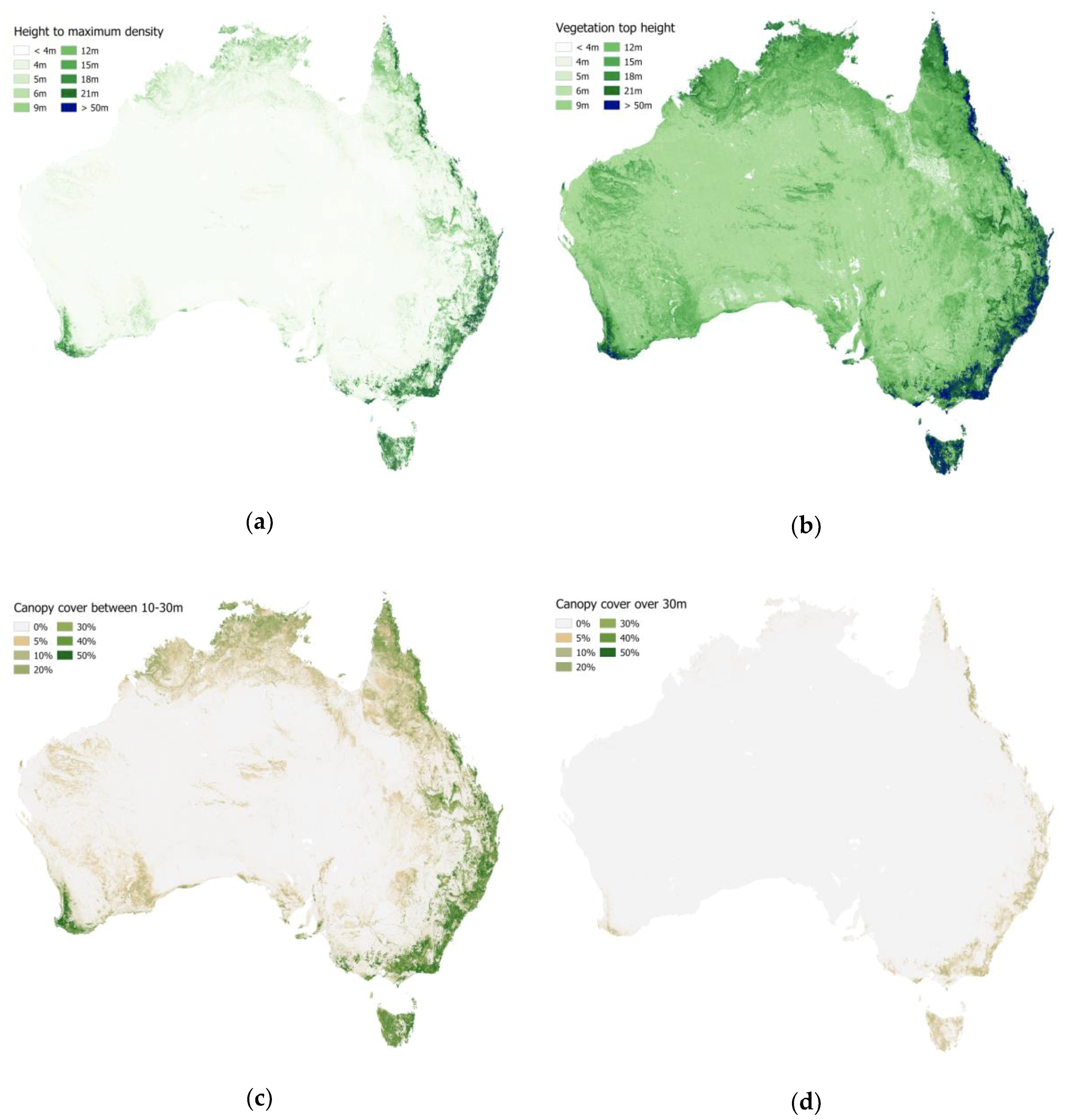
4.1. Height and Cover Maps

Based on the correspondence between the ICESat canopy height metrics assigned to segments generated from ALOS PALSAR and Landsat FPC and independent measures, a map of canopy height was generated at the national level (Figure 8). The highest forests (up to and sometimes exceeding 60 m) were associated with forests in the wetter and more mountainous and/or coastal areas of Tasmania, Victoria, New South Wales, and Queensland. Tall forests were also located in southwestern Australia. The majority of woodlands were less than 25 m in height and occurred throughout the semi-arid zones. The corresponding percentage cover estimates as a function of height class are shown in Figure 8.

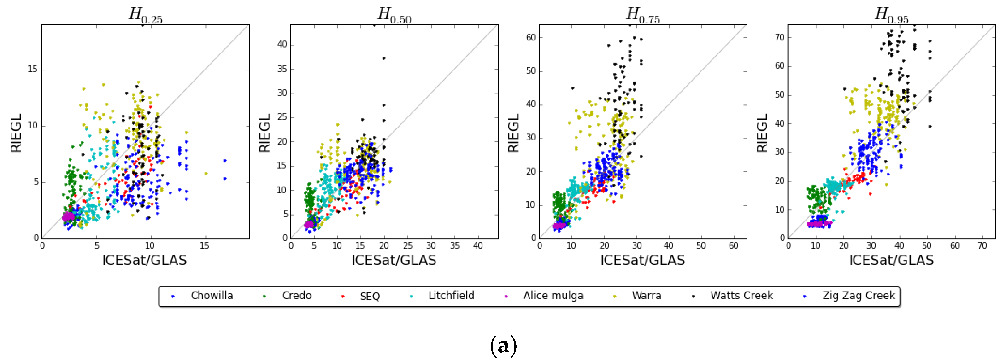
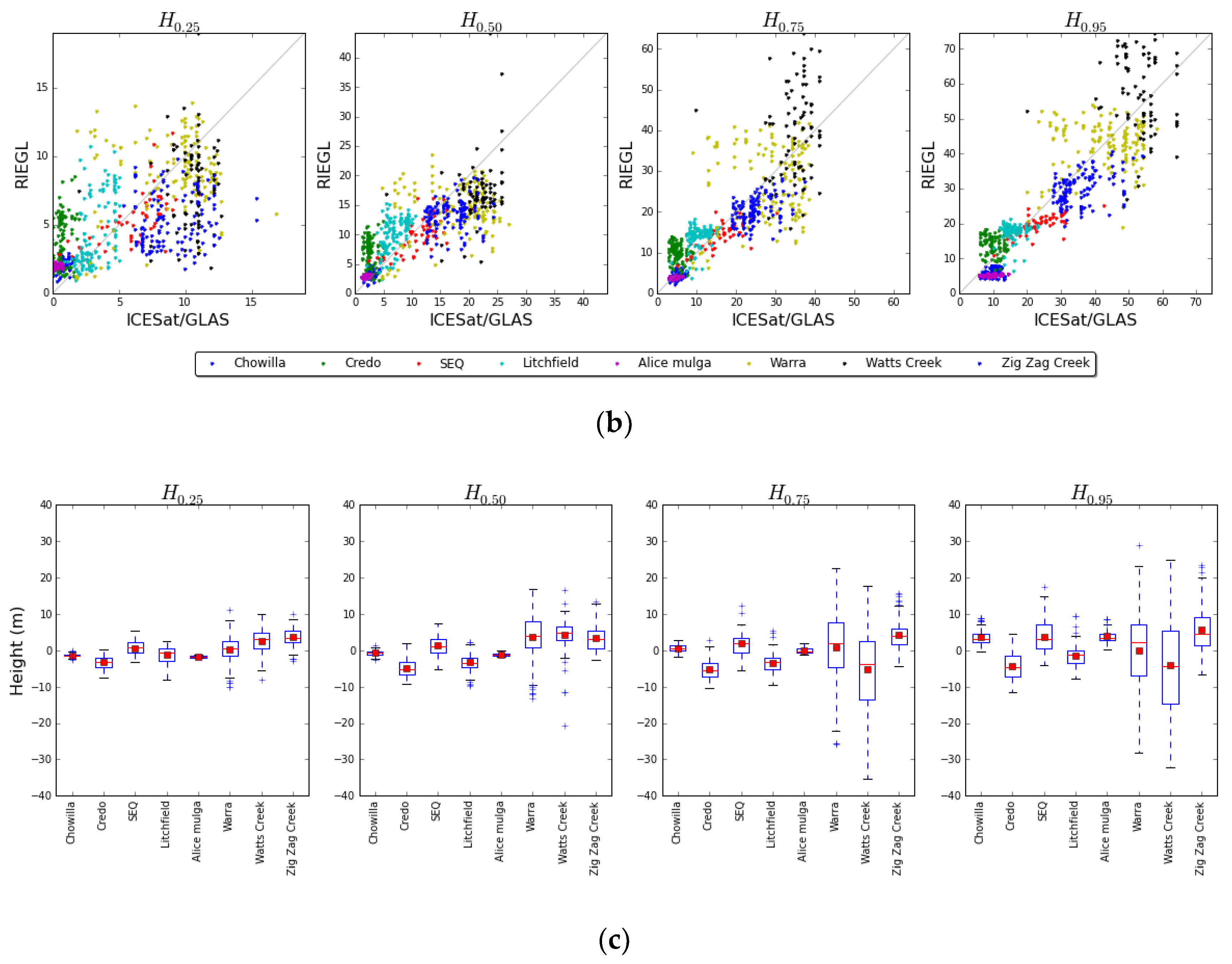
4.2. Comparison with Airborne LiDAR Products

Example RIEGL airborne waveform LiDAR output data products used to generate and compare vertical cover profiles at the TERN Auscover sites are shown for Karawatha forest site in Southeast Queensland in Figure 9. The spatial variations in the apparent reflectance (${\rho }_v \mathrm{and} {\rho }_g)$ shown in Figure 9a,b) were accounted for in the estimation of vertical cover profiles (1 − $P_{gap}\left(\mathsf{\theta },\mathrm{z}\right)$; Figure 9c) and derived height metrics equivalent to those derived from ICESat/GLAS (Figure 9d–f).

The comparison of height metrics (0.25, 0.50, 0.75, and 0.95 percentiles) derived from the segment vertical cover profiles (Figure 10) indicated substantial variation within individual TERN Auscover sites. However, on average these were <10 m (Figure 11c) for the largest height percentile (0.95). Comparison of Figure 10a,b demonstrates that the height metric bias correction reduced the absolute mean differences between the RIEGL and ICESat/GLAS estimates of height percentiles. This was particularly the case for the 0.95 height percentile for the taller forests (Warra and Watts Creek) where there was >10 m reduction in mean absolute difference and final mean differences of <5 m. Across all the TERN Auscover sites, the relative differences were lowest in the upper canopy height metrics (0.75 and 0.95 percentile). The Pearson correlation coefficient between the REIGL and ICESat/GLAS metrics was greatest for the 0.95 percentile (>0.7).

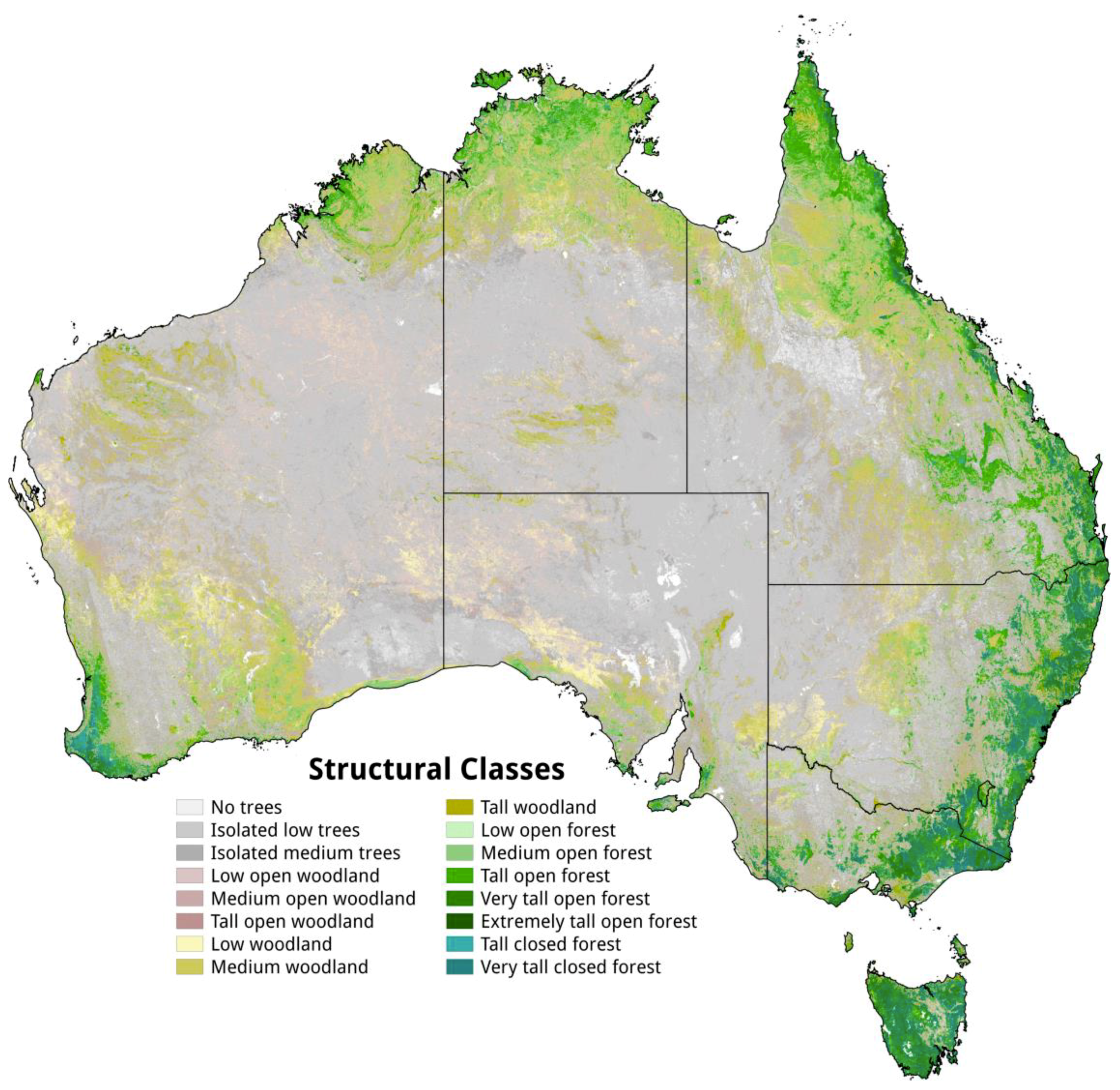
4.3. Structural Formation Map

The 30 m spatial resolution forest structural map for Australia generated by cross tabulating the ICESat/GLAS 0.95 percentile height and total plant cover fraction estimates is shown in Figure 11. Following Table 1, the ICESat/GLAS total plant cover fraction was assumed to be equal to the overstorey crown cover. A 1:1 relationship between LiDAR plant cover and crown cover has been observed for a subset of Australian plant stands by Fisher et al. [34]. However, the generality of this relationship needs further examination over a larger number of sites. The ICESat/GLAS 0.95 percentile heights at 9 and 28 m were assumed to be equivalent to the NVIS 10 m and 30 m height thresholds for the medium and tall woodland/forest categories, respectively.

The map provides considerably more spatial detail compared to the historical classifications generated previously by Specht [15], Carnahan [16], and the NVIS [17] as variability at the pixel and object level (through integration of the Landsat sensor products and ALOS PALSAR data) of height metrics from the ICESat/GLAS is captured by the product. Furthermore, users are able to a directly access information on the vertical structure of woody vegetation as derived from the ICESat/GLAS profiles associated with each class.

As expected, most (82%) of the forests in Australia were associated with the woodland and isolated tree classes and were largely confined to the interior with taller closed forests located predominantly around the coastal regions of eastern Australia, Tasmania, and southwestern Australia (

Table 3. Area (km²) of forests and woodlands of different structural formations, Australia. These structural formations are adapted from the NVIS [17] classes, as described in Table 1.

Structural Formation	Percentage of Total Area	Area ('000s km2)
no trees	3.8%	290
low isolated trees	16.6%	1274
isolated trees	4.9%	379
low open woodland	32.6%	2510
open woodland	20.2%	1552
tall open woodland	0.0%	2
low woodland	0.4%	27
woodland	14.3%	1102
tall woodland	0.1%	5
open forest	4.7%	362
tall open forest	2.3%	179
closed forest	0.1%	10
tall closed forest	0.0%	0
		Total: 7692

). The area of structural formation classes are different to those previously reported by Specht [15], Carnahan [16], and the NVIS [17] due to:

• The height and cover of dryland woody vegetation (woodland and isolated trees classes) are better represented in the products generated in this study, which was supported by the validation of ALS products (e.g. detection of low trees at the Alice Mulga TERN Auscover site; see Figure 10). This translates into greater extent in the structural formation map, which is also consistent with the findings of Bastin et al. [35].
• This study has used SAR and vegetation cover datasets that were only recently available at the national level, and were resampled to 30 m resolution for segmentation in this study. The resulting fine scale of this data product, compared to Spectht [15], Carnahan [16], and the NVIS [17], will also contribute to the difference in areal extents, particularly for forest classes which are often small and patchy across the landscape and may include riparian areas.
• There is considerable uncertainty introduced by thresholding, since a small change in a height and cover threshold may lead to a large change in areal extent for a given class. The use of ICESat data, while leading to an improved product, is not optimized for vegetation and may limit the detection of low vegetation (<5 m) and differentiation between classes. The smaller footprint of the upcoming NASA GEDI instrument (~25 m) will reduce this uncertainty.

5. Discussion

5.1. Segmentation and Classification of the Landscape

Several studies (e.g., [36,37,38]) have highlighted the benefits of integrating data from spaceborne optical sensors, SAR and/or ICESat for better characterization of forests. However, this is the first to demonstrate the use of the combination of all three datasets at a spatial resolution (30 m) that is appropriate for resolving detail at a management scale within the landscape. The segmentation and subsequent classification of the landscape benefits from the use of the Landsat FPC and the ALOS PALSAR L-HV and L-HH, with these channels broadly relating to the amount of foliage (and the small branches that support these), the larger branches within the canopy volume and the trunks respectively. By using these three channels in the segmentation and classification process, areas that are similar in terms of their overall structure are more likely to be captured. Whilst other studies have used segmentation and gridding approaches [9,10], these have focused primarily on the use of optical remote sensing and ancillary data and often do not consider the different structures associated with the woody components. The option to include a digital elevation model (DEM) to build derived measures (e.g., slope; [7]) was not followed, as the terrain is relatively level across much of Australia with minimal surface variation but warrants consideration in future updates of the mapping. However, the SRTM data was effective in removing those returns that were biased as a consequence of slope effects and their inclusion in hillier terrain should be considered.

The height metrics obtained from the airborne LiDAR data agreed with those obtained from the ICESat across a wide range of landscapes, with substantial improvement provided by the height metric bias correction. These results give confidence that the waveforms and derived metrics could be extrapolated across the landscape. The difficulty with the comparison between the airborne LiDAR and the segmented landscape was one of height metric accuracy at the ICESat footprint scale and the trade-off between the number of segment clusters and precision of height estimates across the range of vegetation structural formations across Australia. It is anticipated that, in the future, the greater availability of smaller footprint spaceborne LiDAR with denser spatial sampling will improve both accuracy and precision.

5.2. Vertical Profiles as a Function of Forest Type

Within this study, height metrics retrieved included the 50th, 75th, and 95th percentiles as well as mean height and the height to maximum vegetation density. However, such metrics have proved difficult to obtain, particularly for savannas and other less dense vegetation. This has been attributed to their short height compared to many closed canopy forests. Furthermore, the power of the canopy return is reduced and the contribution from sloped terrain is increased [7]. Lee et al. [28] also noted that waveform extent and vegetation height were underestimated, with the latter by as much as 15 m for very sparse and also dense forests because of saturation in the dense canopy and at the ground respectively. The retrieval of heights in this study was however successful in many woodland areas as the slopes were generally <10°, trees (emergents) were as tall as or exceeding 60 m (with the majority being <20 m), and the canopy cover was relatively low (between 20% and 70%).

The consistency of the waveforms within segments across the class range reflected the ability of the segmentation applied to Landsat FPC and ALOS PALSAR HH and HV data to define the extent of forests with similar structural characteristics. The vertical profiles extracted from the ICESat data could also be interpreted in relation to the forest type as well as growth stage. For example, within forests that had remained relatively undisturbed since European settlement [39] and which had received minimal natural interference since the late 1980s (i.e., were regarded as remnant), layering within the vertical profile was observed. These profiles differed for both open and closed forests, with this reflecting the variable amounts of plant material within the vertical profile. Where a multi-layered profile with a distinct regrowth layer was observed, disturbance events (e.g., fires, selective logging) were suggested. Regrowth forests were typically single layered and of relatively low stature, but the profiles often showed the influence of a small number of emergent trees still existing within the mapped segments.

5.3. Comparison with Other Studies

Estimates of forest canopy height have been generated previously by Lefsky [10], Simard et al. [11], and Scarth et al. [40] and extracts were compared to those generated in this study in Figure 12. With the map generated by [40], each of the RE units was associated with a canopy height estimate derived from the LiDAR. However, only those polygons associated with remnant vegetation were analyzed and disturbance within remnant areas (e.g., through wildfires) was not considered. In retrieving and extrapolating height estimates, [11] used a grid-based system and assigned height metrics according to the Land Processes Distributed Active Archive Centre (LP DAAC) MODIS land cover categories. The study of [10] similarly used a segmentation of the MODIS data but only referenced profiles from tropical broadleaf forests in Brazil, temperate broadleaf forests in Tennessee, and temperate needleleaf forests. For Australia, the height map generated in this study was most comparable to that generated by [11]. The previous map of [40] omitted large areas because of the focus on remnant ecosystems (RE) only, omitting large areas of regenerating woody vegetation. The map of [10] omitted large areas of forest as the study did not detect the lower stature (typically <20 m) trees associated with more open forests and woodlands [7].

5.4. Wider Applications

Whilst the generation of the Landsat FPC has allowed estimates of vegetation cover to be produced at moderate (<30 m) spatial resolution, reliable retrieval of canopy height and the distribution of plant material within the vertical profile has remained a significant challenge [40]. The methods conveyed in this paper demonstrate, for the first time, a robust approach to retrieval of a range of height metrics and descriptors across the landscape. Additional information (e.g., on biomass levels) can also be provided through reference to the ALOS PALSAR L-HH and L- HV data [21]. The combination of the derived products (cover, height and, in the latter case, biomass) has significant potential to facilitate the establishment of better baseline estimates of carbon stocks and changes in these as a consequence of clearance or wildfires, with these able to be mapped using time-series of Landsat sensor data. In terms of biodiversity, knowledge of the height and dimensions and number of layers within the forest column is important for assessment purposes, particularly given that many studies have found a close link between species richness (e.g., of birds, reptiles) and forest height [41]. The datasets generated address the requirement for information on essential biodiversity variables (EBVs), namely height, cover, and above ground biomass [42]. The integration of the three datasets also facilitates a better interpretation of these, which benefits future users in gaining and understanding of how these can be exploited for a range of applications.

It is important to note that this is a demonstration product developed under the auspices of the JAXA Kyoto & Carbon Initiative, and therefore should be independently evaluated before use in operational environmental monitoring programs. The approach using segmentation and imputation is simple and may be applied to data from the upcoming confluence of active remote sensing instruments designed for vegetation measurement (e.g. NASA’s GEDI and NISAR) to reduce uncertainties in height and cover retrievals, and subsequently aboveground biomass mapping.

6. Conclusions

This study has established and applied a method for characterizing the height profiles of woody vegetation across Australia from ICESat data, with this benefiting from the segmentation of the ALOS PALSAR L-band HH and HV data and Landsat-derived FPC and clustering of the segments into distinct structural classes. The approach extracted vegetation profiles from segments with available ICESat data and then extrapolated these to other segments assigned to the same class. The accuracies of retrieval for canopy profiles and metrics (e.g., height) were at an acceptable level and profiles were similar within segments of the same class. The maps provided a better representation of the known distribution of stand heights compared to those generated previously. As ALOS PALSAR, Landsat sensor and ICESat data were available across Australia, the approach was applied nationally and the resulting data products have been made openly available (http://dx.doi.org/10.4227/05/5703458340442). The approach can also be applied subsequently to ALOS-2 PALSAR-2 (and in future NISAR), Landsat or Sentinel-2-derived FPC or persistent green vegetation cover and from 2019 the Global Ecosystem Dynamics Investigation (GEDI) and ICESat-2 data, which we anticipate will considerably reduce uncertainty in the vertical cover profile mapping and derived products. Once generated, a wide range of applications relating to carbon budgeting and science, biodiversity assessment and conservation, and better forest management are anticipated.

References

1. Fatoyinbo, T.E.; Simard, M. Height and biomass of mangroves in Africa from ICESat/GLAS and SRTM. Int. J. Remote Sens. 2013, 34, 668–681. [Google Scholar] [CrossRef]
2. Walker, W.S.; Kellndorfer, J.M.; Pierce, L.E. Quality assessment of SRTM C- and X-band interferometric data: Implications for the retrieval of vegetation canopy height. Remote Sens. Environ. 2007, 106, 428–448. [Google Scholar] [CrossRef]
3. Boudreau, J.; Nelson, R.; Margolis, H.; Beaudoin, A.; Guindon, L.; Kimes, D. Regional aboveground forest biomass using airborne and spaceborne LiDAR in Québec. Remote Sens. Environ. 2008, 112, 3876–3890. [Google Scholar] [CrossRef]
4. Nelson, R.; Boudreau, J.; Gregoire, T.G.; Margolis, H.; Næsset, E.; Gobakken, T.; Ståhl, G. Estimating Quebec provincial forest resources using ICESat/GLAS. Can. J. For. Res. 2009, 39, 862–881. [Google Scholar] [CrossRef]
5. Wulder, M.A.; White, J.C.; Nelson, R.F.; Næsset, E.; Ørka, H.O.; Coops, N.C.; Hilker, T.; Bater, C.W.; Gobakken, T. Lidar sampling for large-area forest characterization: A review. Remote Sens. Environ. 2012, 121, 196–209. [Google Scholar] [CrossRef] [Green Version]
6. Nelson, R.; Ranson, K.J.; Sun, G.; Kimes, D.S.; Kharuk, V.; Montesano, P. Estimating Siberian timber volume using MODIS and ICESat/GLAS. Remote Sens. Environ. 2009, 113, 691–701. [Google Scholar] [CrossRef]
7. Kellndorfer, J.M.; Walker, W.S.; LaPoint, E.; Kirsch, K.; Bishop, J.; Fiske, G. Statistical fusion of lidar, InSAR, and optical remote sensing data for forest stand height characterization: A regional-scale method based on LVIS, SRTM, Landsat ETM+, and ancillary data sets. J. Geophys. Res. Biogeosci. 2010. [Google Scholar] [CrossRef]
8. Ørka, H.O.; Wulder, M.A.; Gobakken, T.; Næsset, E. Integrating airborne laser scanner data and ancillary information for delineating the boreal–alpine transition zone in Hedmark County, Norway. In Proceedings of the Proceedings of SilviLaser, Freiburg, Germany, 14–17 September 2010. [Google Scholar]
9. Los, S.O.; Rosette, J.A.B.; Kljun, N.; North, P.R.J.; Chasmer, L.; Suárez, J.C.; Hopkinson, C.; Hill, R.A.; van Gorsel, E.; Mahoney, C.; et al. Vegetation height and cover fraction between 60° S and 60° N from ICESat GLAS data. Geosci. Model Dev. 2012, 5, 413–432. [Google Scholar] [CrossRef] [Green Version]
10. Lefsky, M.A. A global forest canopy height map from the Moderate Resolution Imaging Spectroradiometer and the Geoscience Laser Altimeter System. Geophys. Res. Lett. 2010. [Google Scholar] [CrossRef]
11. Simard, M.; Pinto, N.; Fisher, J.B.; Baccini, A. Mapping forest canopy height globally with spaceborne lidar. J. Geophys. Res. 2011. [Google Scholar] [CrossRef]
12. Chi, H.; Sun, G.; Huang, J.; Guo, Z.; Ni, W.; Fu, A. National Forest Aboveground Biomass Mapping from ICESat/GLAS Data and MODIS Imagery in China. Remote Sens. 2015, 7, 5534–5564. [Google Scholar] [CrossRef] [Green Version]
13. Gill, T.; Johansen, K.; Phinn, S.; Trevithick, R.; Scarth, P.; Armston, J. A method for mapping Australian woody vegetation cover by linking continental-scale field data and long-term Landsat time series. Int. J. Remote Sens. 2017, 38, 679–705. [Google Scholar] [CrossRef]
14. An Interim Biogeographic Regionalisation for Australia: A Framework for Setting Priorities in the National Reserves System Cooperative Program; Thackway, R.; Cresswell, I.; Australian Nature Conservation Agency (Eds.) Version 4.0; Australian Nature Conservation Agency, Reserve Systems Unit: Canberra, Australia, 1995; ISBN 978-0-642-21371-6. [Google Scholar]
15. Specht, R.L. Vegetation. In Leeper, G.W. (ed.), “Australian Environment”; Melbourne University Press: Melbourne, Australia, 1970; pp. 44–67. [Google Scholar]
16. Carnahan, J.A. Natural Vegetation. In Atlas of Australian Resources; Second Series; Department of Natural Resources: Canberra, Australia, 1976. [Google Scholar]
17. Department of the Environment and Water Resources. Australia’s Native Vegetation: A Summary of Australia’s Major Vegetation Groups; Australian Government: Canberra, Australia, 2007. [Google Scholar]
18. Specht, R.L.; Specht, A. Australian plant communities: dynamics of structure, growth and biodiversity; Oxford University Press: Melbourne, Australia, 2000. [Google Scholar]
19. Walker, J.; Hopkins, M.S. Vegetation. In Australian Soil and Land Survey: Field Handbook; Inkata Press: Melbourne, Australia, 1990. [Google Scholar]
20. Shimada, M.; Ohtaki, T. Generating Large-Scale High-Quality SAR Mosaic Datasets: Application to PALSAR Data for Global Monitoring. IEEE J. Sel. Top. Appl. Earth Obs. Remote Sens. 2010, 3, 637–656. [Google Scholar] [CrossRef]
21. Lucas, R.; Armston, J.; Fairfax, R.; Fensham, R.; Accad, A.; Carreiras, J.; Kelley, J.; Bunting, P.; Clewley, D.; Bray, S. An evaluation of the ALOS PALSAR L-band backscatter—Above ground biomass relationship Queensland, Australia: Impacts of surface moisture condition and vegetation structure. IEEE J. Sel. Top. Appl. Earth Obs. Remote Sens. 2010, 3, 576–593. [Google Scholar] [CrossRef]
22. Clewley, D.; Bunting, P.; Shepherd, J.; Gillingham, S.; Flood, N.; Dymond, J.; Lucas, R.; Armston, J.; Moghaddam, M. A python-based open source system for geographic object-based image analysis (GEOBIA) utilizing raster attribute tables. Remote Sensss. 2014, 6, 6111–6135. [Google Scholar] [CrossRef]
23. Shephard, J.; Bunting, P.; Dymond, J. Operational large-scale segmentation of imagery based on iterative elimination. Remote Sens. Submitted.
24. Lucas, R.M.; Moghaddam, M.; Cronin, N. Microwave scattering from mixed-species forests, Queensland, Australia. IEEE Trans. Geosci. Remote Sens. 2004, 42, 2142–2159. [Google Scholar] [CrossRef]
25. Pedregosa, F.; Varoquaux, G.; Gramfort, A.; Michel, V.; Thirion, B.; Grisel, O.; Blondel, M.; Prettenhofer, P.; Weiss, R.; Dubourg, V.; et al. Scikit-learn: Machine Learning in Python. J. Mach. Learn. Res. 2011, 12, 2825–2830. [Google Scholar]
26. Ketchen, D.J.; Shook, C.L. The application of cluster analysis in strategic management research: An analysis and critique. Strateg. Manag. J. 1996, 17, 441–458. [Google Scholar] [CrossRef]
27. Lefsky, M.A.; Harding, D.J.; Keller, M.; Cohen, W.B.; Carabajal, C.C.; Bom, F.D.; Hunter, M.O.; Oliveira, R.J. de Estimates of forest canopy height and aboveground biomass using ICESat. Geophys. Res. Lett. 2005, 32, 1–4. [Google Scholar] [CrossRef]
28. Lee, S.; Ni-Meister, W.; Yang, W.; Chen, Q. Physically based vertical vegetation structure retrieval from ICESat data: Validation using LVIS in White Mountain National Forest, New Hampshire, USA. Remote Sens. Environ. 2011, 115, 2776–2785. [Google Scholar] [CrossRef]
29. Nelson, R. Model effects on GLAS-based regional estimates of forest biomass and carbon. Int. J. Remote Sens. 2010, 31, 1359–1372. [Google Scholar] [CrossRef] [Green Version]
30. Rosette, J.A.B.; North, P.R.J.; Suárez, J.C.; Los, S.O. Uncertainty within satellite LiDAR estimations of vegetation and topography. Int. J. Remote Sens. 2010, 31, 1325–1342. [Google Scholar] [CrossRef]
31. Johansen, K.; Trevithick, R.; Bradford, M.; Hacker, J.; McGrath, A.; Lieff, W. Australian examples of field and airborne TERN Landscape Assessment campaigns. In Effective Field Calibration and Nalidation Practices: A Practical Handbook for Calibration and Validation of Satellite and Model-Derived Terrestrial Environmental Variables for Research and Management; Held, A., Phinn, S., Soto-Berrelov, M., Jones, S., Eds.; TERN Auscover: Canberra, Australia, 2018; ISBN 978-0-646-94137-0. [Google Scholar]
32. Armston, J.; Disney, M.; Lewis, P.; Scarth, P.; Phinn, S.; Lucas, R.; Bunting, P.; Goodwin, N. Direct retrieval of canopy gap probability using airborne waveform lidar. Remote Sens. Environ. 2013, 134, 24–38. [Google Scholar] [CrossRef]
33. Garcia, D. Robust smoothing of gridded data in one and higher dimensions with missing values. Comput. Stat. Data Anal. 2010, 54, 1167–1178. [Google Scholar] [CrossRef] [Green Version]
34. Fisher, A.; Scarth, P.; Armston, J.; Danaher, T. Relating foliage and crown projective cover in Australian tree stands. Agric. For. Meteorol. 2018, 259, 39–47. [Google Scholar] [CrossRef]
35. Bastin, J.-F.; Berrahmouni, N.; Grainger, A.; Maniatis, D.; Mollicone, D.; Moore, R.; Patriarca, C.; Picard, N.; Sparrow, B.; Abraham, E.M.; et al. The extent of forest in dryland biomes. Science 2017, 356, 635. [Google Scholar] [CrossRef] [PubMed]
36. Dolan, K.; Masek, J.G.; Huang, C.; Sun, G. Regional forest growth rates measured by combining ICESat GLAS and Landsat data. J. Geophys. Res. Biogeosci. 2009. [Google Scholar] [CrossRef]
37. Mitchell, A.L.; Tapley, I.; Milne, A.K.; Williams, M.L.; Zhou, Z.-S.; Lehmann, E.; Caccetta, P.; Lowell, K.; Held, A. C- and L-band SAR interoperability: Filling the gaps in continuous forest cover mapping in Tasmania. Remote Sens. Environ. 2014, 155, 58–68. [Google Scholar] [CrossRef]
38. Lucas, R.M.; Clewley, D.; Accad, A.; Butler, D.; Armston, J.; Bowen, M.; Bunting, P.; Carreiras, J.; Dwyer, J.; Eyre, T. Mapping forest growth and degradation stage in the Brigalow Belt Bioregion of Australia through integration of ALOS PALSAR and Landsat-derived foliage projective cover data. Remote Sens. Environ. 2014, 155, 42–57. [Google Scholar] [CrossRef] [Green Version]
39. Regional Ecosystems Descriptions—Methodology for Survey and Mapping of Regional Ecosystems and Vegetation Communities—Publications | Queensland Government Available online:. Available online: https://publications.qld.gov.au/dataset/redd/resource/6dee78ab-c12c-4692-9842-b7257c2511e4 (accessed on 5 August 2018).
40. Scarth, P.; Armston, J.; Goodwin, N. If You Climb Up A Tree, You Must Climb Down The Same Tree. But How High Was It? Available online: https://search.datacite.org/works/10.6084/m9.figshare.94251.v1 (accessed on 5 August 2018).
41. Bowen, M.E.; McAlpine, C.A.; House, A.P.N.; Smith, G.C. Agricultural landscape modification increases the abundance of an important food resource: Mistletoes, birds and brigalow. Biol. Conserv. 2009, 142, 122–133. [Google Scholar] [CrossRef]
42. Pereira, H.M.; Ferrier, S.; Walters, M.; Geller, G.N.; Jongman, R.H.G.; Scholes, R.J.; Bruford, M.W.; Brummitt, N.; Butchart, S.H.M.; Cardoso, A.C.; et al. Essential Biodiversity Variables. Science 2013, 339, 277–278. [Google Scholar] [CrossRef] [PubMed] [Green Version]
Figure 1. An overview of vegetation in the Australian landscape, as adapted from the National Vegetation Inventory System (NVIS) [17] (30 m spatial resolution, EPSG:3577 Australian Albers projection).
Remotesensing 11 00147 g001
Figure 2. Composite of Landsat foliage projective cover (FPC), ALOS PALSAR L-band HH and HV data for Australia (30 m spatial resolution, EPSG:3577 Australian Albers projection) in red, green, and blue (RGB) overlain with ICESat/GLAS footprints (yellow).
Remotesensing 11 00147 g002
Figure 3. Overview of the processing of ALOS PALSAR HH and HV, Landsat-derived foliage projective cover (FPC) and ICESat/GLAS data.
Remotesensing 11 00147 g003
Figure 4. Tiled segmentation of (a) an L-HH, L-HV, and Landsat-derived foliage projective cover (FPC) composite for Australia using the approach outlined by Clewley et al. [22], with this producing (b) with >33 million segments. Examples of the segmentation for (c) tropical savanna woodlands in northern Queensland with relatively low FPC but high L-HV showing as green and (d) areas of evergreen pasture in Victoria showing as blue with low L-HH and L-HV but high FPC. The locations of (c) and (d) are shown as red boxes in (a). The ALOS PALSAR data are © JAXA/METI.
Remotesensing 11 00147 g004
Figure 5. Plot of the percentage of variance explained as a function of the number of clusters used to determine the optimal number of clusters. 1000 clusters were selected through visual inspection of the classification.
Remotesensing 11 00147 g005
Figure 6. Comparison of ICESat footprints from slopes > 5° (left) and < 5° (right). Dashed red waveforms are from slopes > 5°. Dotted red waveforms are from slopes < 5°. Green lines represent the mean return for the cluster.
Remotesensing 11 00147 g006
Figure 7. The relationship between the cluster fitted ground standard deviation and the calculated 95th percentile height (left) shows a distinct relationship. By correcting the height using Equation (6), bias in the height estimation was removed (right).
Remotesensing 11 00147 g007
Figure 8. Maps (30 m spatial resolution) of vegetation height at (a) top of canopy and (b) at 10 m and canopy cover at (c) 10–30 m and (d) >30 m for Australia. These data layers were generated by assigning ICESat vertical height information and Landsat-derived foliage projective cover (FPC) to segments.
Remotesensing 11 00147 g008
Figure 9. Example RIEGL airborne waveform LiDAR output data products for the TERN Auscover Karawatha forest site in Southeast Queensland. These were used for validation of ICESat/GLAS vertical cover profiles and derived height metrics at the segment level.
Remotesensing 11 00147 g009
Figure 10. Comparison of RIEGL and ICESat/GLAS height metrics (0.25, 0.50, 0.75, and 0.95 percentiles) derived from vertical cover profiles for each segment across the TERN Auscover sites. (a) without height metric bias correction; (b) with height metric bias correction across the TERN Auscover sites. The distributions of RIEGL and ICESat/GLAS height metric differences for each of the sites are shown in (c).
Remotesensing 11 00147 g010aRemotesensing 11 00147 g010b
Figure 11. Forest structural formation classification of Australia generated in this study. These structural formations are adapted from Australia’s National Vegetation Information System (NVIS) [17] classes, as described in Table 1.
Remotesensing 11 00147 g011
Figure 12. Estimates of vegetation height for Queensland, Australia, based on (a) Scarth et al. [40], (b) Simard et al. [11], and (c) this study.
Remotesensing 11 00147 g012